
An Optimized Core Distribution Adaptive Topology Reconfiguration Algorithm for NoC-Based Embedded Systems

Abstract
1. Introduction
- (1)
- (2)
- Coordinate Systems: Circulant virtual coordinate frameworks decouple logical addressing from physical failures, enabling resilient rerouting independent of defective components [16];
- (3)
- Topology Design: Architectural redundancy through spare cores or reconfigurable interconnects preemptively mitigates fault propagation [17].
2. Related Works
- (1)
- They do not adequately take into account the spatial distribution of faulty cores, potentially leading to suboptimal solutions;
- (2)
- They exhibit higher computational complexity and cannot maintain a balance between the topology reconfiguration rate and the topology recovery time;
- (3)
- They could achieve a higher resuccess rate of topology reconfiguration for low-scale, low-fault-rate topology, but it may not be applicable to high-scale, high-fault-rate topology in embedded systems.
- (1)
- We propose an adaptive topology reconfiguration algorithm based on the faulty core distribution mechanism, which effectively improves the success rate of topology reconfiguration;
- (2)
- We propose a search algorithm based on a sliding window after determining the distribution location of the faulty core, which effectively improves the efficiency of the search process and the recovery time of faulty systems.
3. Preliminaries
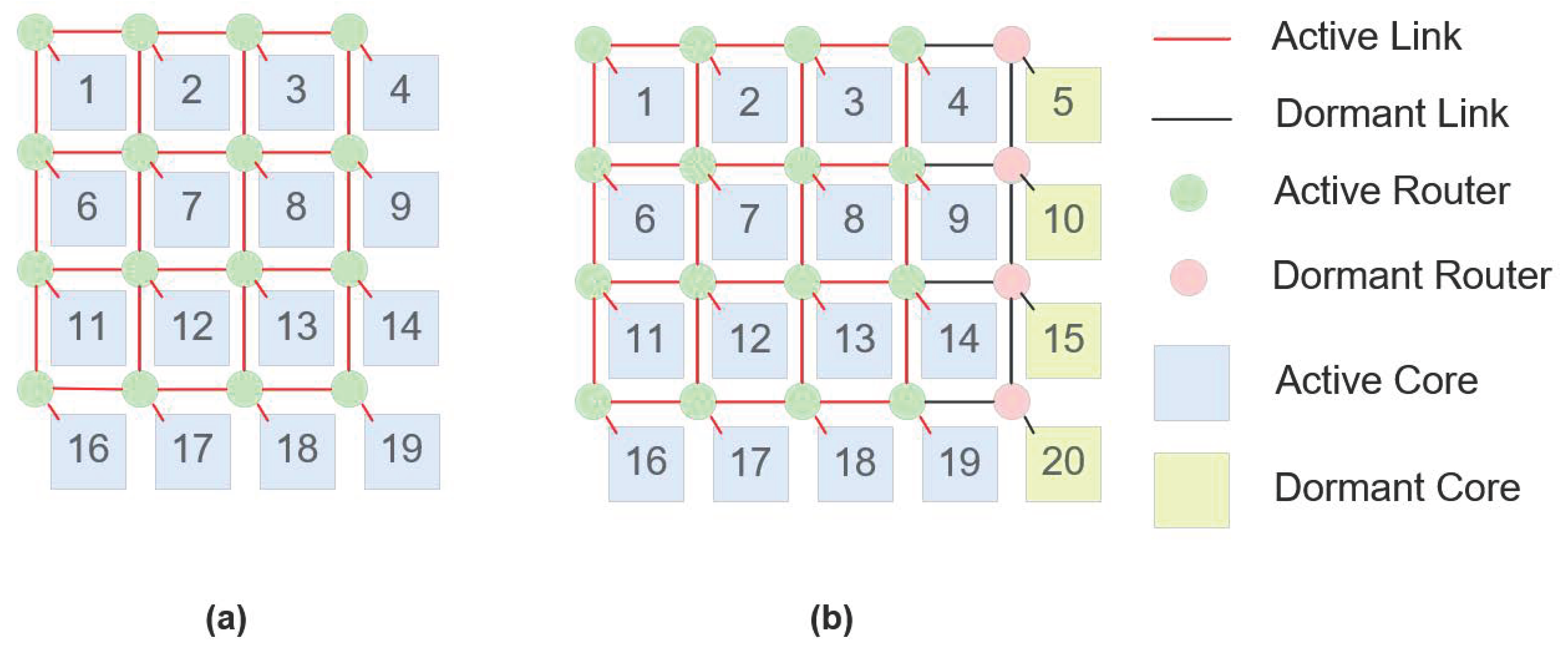
3.1. Two-Dimensional Mesh and 2D REmesh Architecture
- (1)
- Constant Number of Redundant Cores: The 2D REmesh maintains the same number of redundant cores as the conventional 2D mesh, ensuring that the total area occupied by processor cores remains consistent between both structures;
- (2)
- Addition of Routers: To enhance system scalability, the REmesh integrates an additional row and an extra column of routers atop the traditional 2D mesh. The area occupied by a single router is significantly smaller than that of a processor core, and as the network size increases, the proportion of the total area attributed to routers diminishes, rendering the area overhead associated with these additional routers acceptable;
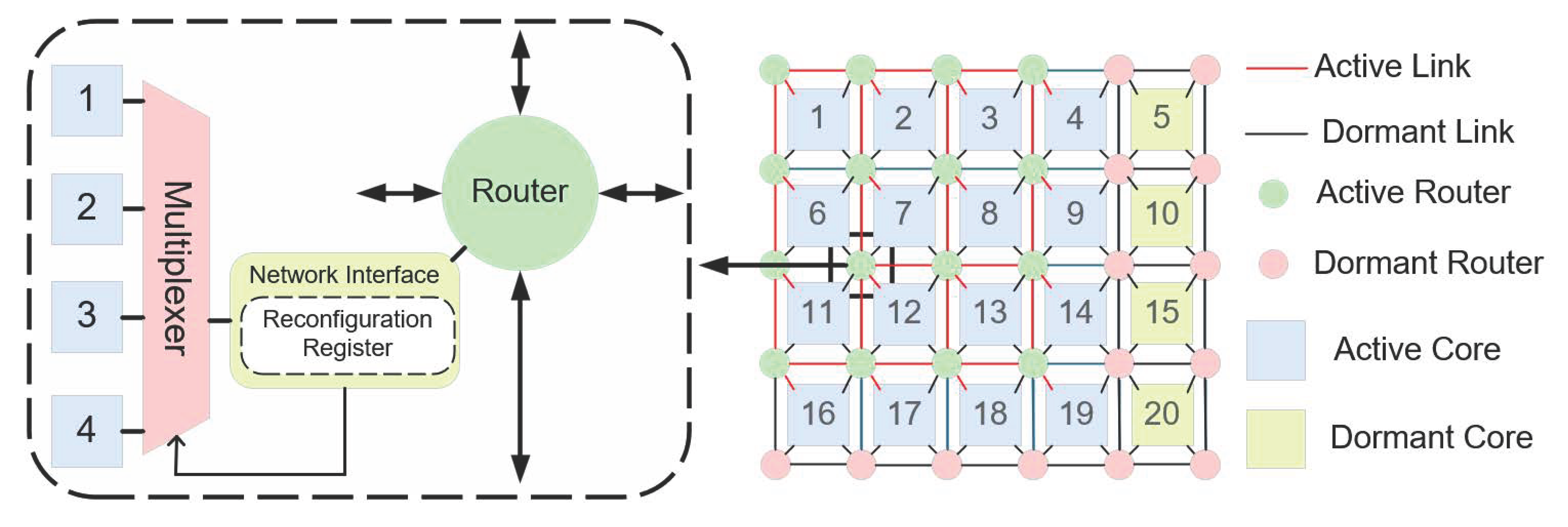
- (3)
- Multiplexer Connectivity: Unlike the fixed connections in a traditional 2D mesh, routers in the 2D REmesh are connected through multiplexers. This arrangement features three router types: corner routers, which connect solely to adjacent cores; edge routers, which can connect to one of two neighboring cores via multiplexers; and interior routers, which can connect to any of the four surrounding cores. By default, each router connects to the lower-right core, facilitating greater flexibility and enabling dynamic restoration of the physical topology;
- (4)
- Enhanced Ports and Connections: The 2D REmesh structure increases overall bandwidth and mitigates data transmission bottlenecks by augmenting the number of ports and connections. This design fosters enhanced scalability, optimized load balancing, and improved flexibility, while providing robust fault tolerance and the capability for topology reconfiguration in the event of faulty cores.
3.2. REmesh Physical Array Architecture and Logical Topology Reconfiguration
3.3. Evaluation Metrics
- (1)
- Successful Reconfiguration Rate (SRR)
- (2)
- Average Recovery Time (ART)
- (3)
- Core Reuse Rate (CRR)
- (4)
- Comprehensive Evaluation Metric (CEM)
4. Problem Formulation
4.1. Mathematical Model of the Proposed Algorithm
- (1)
- The normalized Euclidean distance:
- (2)
- Faulty core distribution factor within the sliding window:
- (3)
- Dynamic threshold:
- (4)
- Number of faulty processing elements (PEs)
- (5)
- Replacement Metric:
- (6)
- Quality Metric:
- (7)
- Utility Function Calculation:
4.2. Mathematical Proof of the Optimal Solution
5. Adaptive Core Distribution Optimization Algorithm
5.1. ACTR Algorithm
- (1)
- Faulty core distribution recognition mechanism:
- (a)
- Faulty cores that are centrally distributed in the upper right corner of the network, referred to as URC cores.
- (b)
- Faulty cores that are centrally distributed in the down left corner of the network, referred to as DLC cores.
- (c)
- Faulty cores that are scattered down in the corner of the network, referred to as SDC cores.
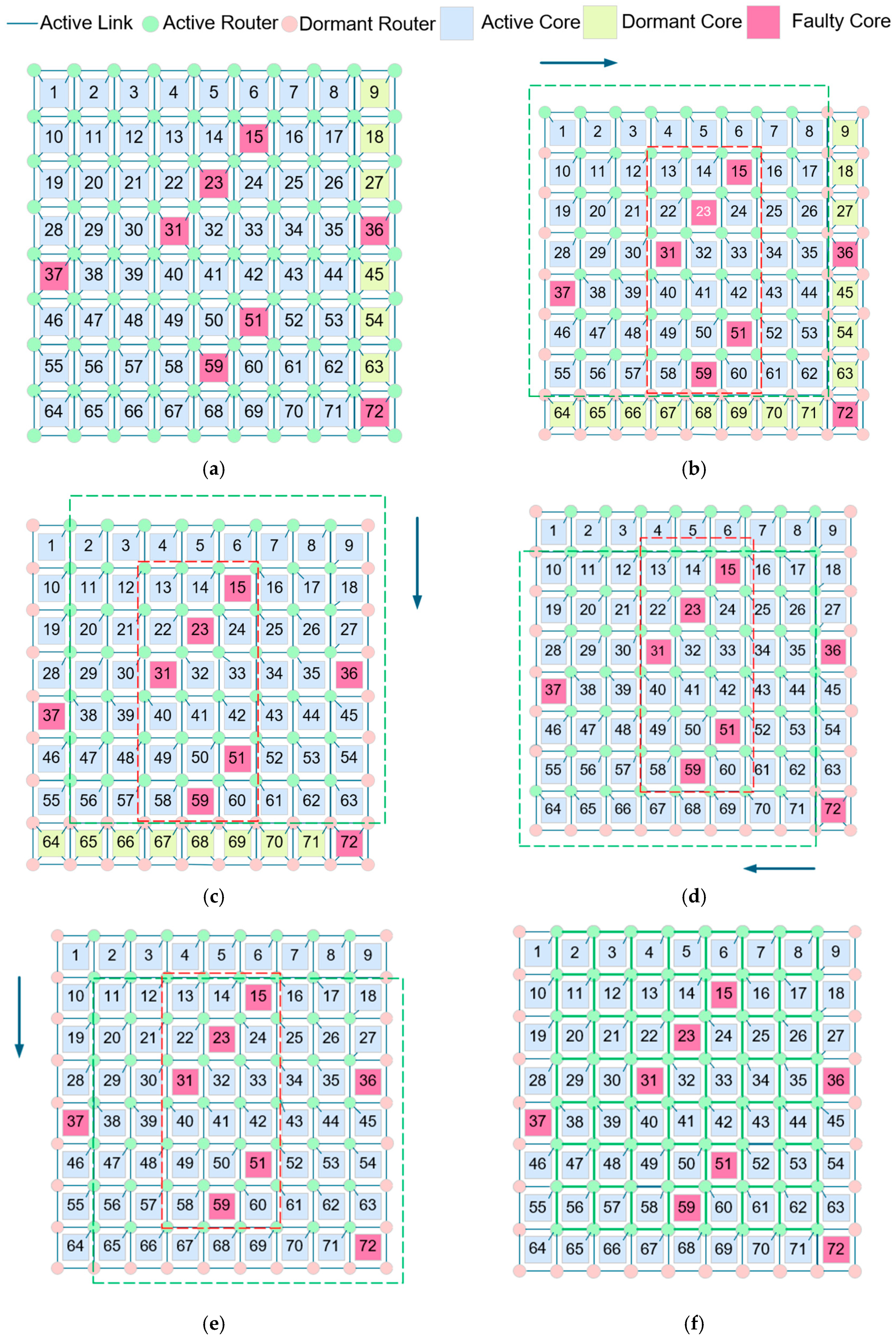
- (2)
- Sliding window search mechanism:
- (a)
- If the faulty cores are centrally distributed in the upper right corner, the search order should be forward sliding clockwise along the y-axis and reverse sliding counterclockwise along the x-axis;
- (b)
- If the faulty cores are concentrated in the lower left corner, the search sequence should be forward sliding clockwise along the x-axis, reverse sliding counterclockwise along the y-axis;
- (c)
- If the faulty cores are scattered, the search order should be forward sliding clockwise along the x-axis and reverse sliding clockwise along the x-axis.
| Algorithm 1. ACTR Algorithm. |
| Input: An physical array H |
| Output: An target array T |
| 1: S := H; |
| 2: Initialize t := 0; |
| 3: for i := 0 to n − 1 do |
| 4: for j := 0 to n − 1 do |
| 5: Pan the routers to generate a new router framework for solution S; |
| 6: end for |
| 7: end for |
| 8: for i := 0 to n − 1 do |
| 9: for j := 0 to n + k − 1 do |
| 10: Find all faulty cores depending on the coordinates in |
| 11: Record the number of faulty PEs; |
| 12: if is faulty then |
| 13: t := t + 1; |
| 14: end if |
| 15: end for |
| 16: end for |
| 17: for i := 0 to t − 1 do |
| 18: for j := i + 1 to t − 1 do /*t representing the number of faulty PEs;*/ |
| 19: Calculate the normalized Euclidean distance of faulty PEs; |
| 20: end for |
| 21: end for |
| 22: Generate the core distribution factor for Q; |
| 23: Dynamic_threshold := ; |
| 24: if Dynamic_threshold >= Q then |
| 25: T := ACTR-SDC(S); |
| 26: return T; |
| 27: end if |
| 28: for i := 0 to t − 1 do |
| 29: Calculate the upper right numbers of faulty PEs in count1; |
| 30: Calculate the lower left numbers of faulty PEs in count2; |
| 31: end for |
| 32: if count1 ≥ count2 then |
| 33: T := ACTR-URC(S); |
| 34: else |
| 35: T := ACTR-DLC(S); |
| 36: end if |
| 37: return T; |
| Algorithm 2. ACTR-URC Procedure. |
| Input: An initial solution generated by ACTR; |
| Output: Optimized search solution |
| 1: := |
| 2: max_iterations :=k |
| 3: iteration_count := 0 |
| 4: := ; |
| 5: while iteration_count < max_iterations do |
| 6: := SDW(); //Update using SDW based on current solution |
| 7: := ; |
| 8: Perform a forward search with searching order sliding clockwise along the y-axis; |
| 9: Perform a reverse search with searching order sliding anticlockwise along the x-axis; |
| 10: if Utility() < Utility() then //Update only if the new configuration is better |
| 11: := ; //Update the best solution |
| 12: end if |
| 13: iteration_count := iteration_count + 1; |
| 14: end while |
| 15: return ; |
| Algorithm 3. SDW Procedure. |
| Input: An physical array H with defect locations D |
| Output: Optimized target array of size |
| 1: Initialize to an empty array; |
| 2: Precompute non-defective PEs positions in H and store in a list N; |
| 3: Initialize a sliding window F of size at the top-left corner of H; |
| 4: Call Sub-SlideWindow(H, F, , D); |
| 5: Procedure Sub-SlideWindow(H, F, , D); |
| 6: for each row i from 0 to m-p do |
| 7: for each column j from 0 to n-q do |
| 8: Move the sliding window F to position (i, j) in H; |
| 9: Initialize currentUtility = 0; //Store utility for the current window configuration |
| 10: for each defect in D do |
| 11: Find the nearest non-defective PEs using precomputed positions in N; |
| 12: Replace the defective PEs with the nearest non-defective PEs; |
| 13: Update currentUtility based on the configuration of F; |
| 14: end for; |
| 15: if currentUtility > then //Update condition corrected for maximization |
| 16: Update to the current configuration of F; |
| 17: end if; |
| 18: end for; |
| 19: end for; |
| 20: if p = q then |
| 21: //Optional: If the target array is square, try rotating the window; |
| 22: Call Sub-SlideWindow(H, F rotated,, D); |
| 23: //Choose the better configuration between the current and the rotated one; |
| 24: Update to the better configuration; |
| 25: end if; |
| 26: return ; |
5.2. Example of Topology Reconfiguration in REmesh NoC
6. Experimental Data Results and Analysis
6.1. Experimental Preparation
6.2. Experimental Research Plan and Methodology
6.3. Experimental Performance Metrics Analysis
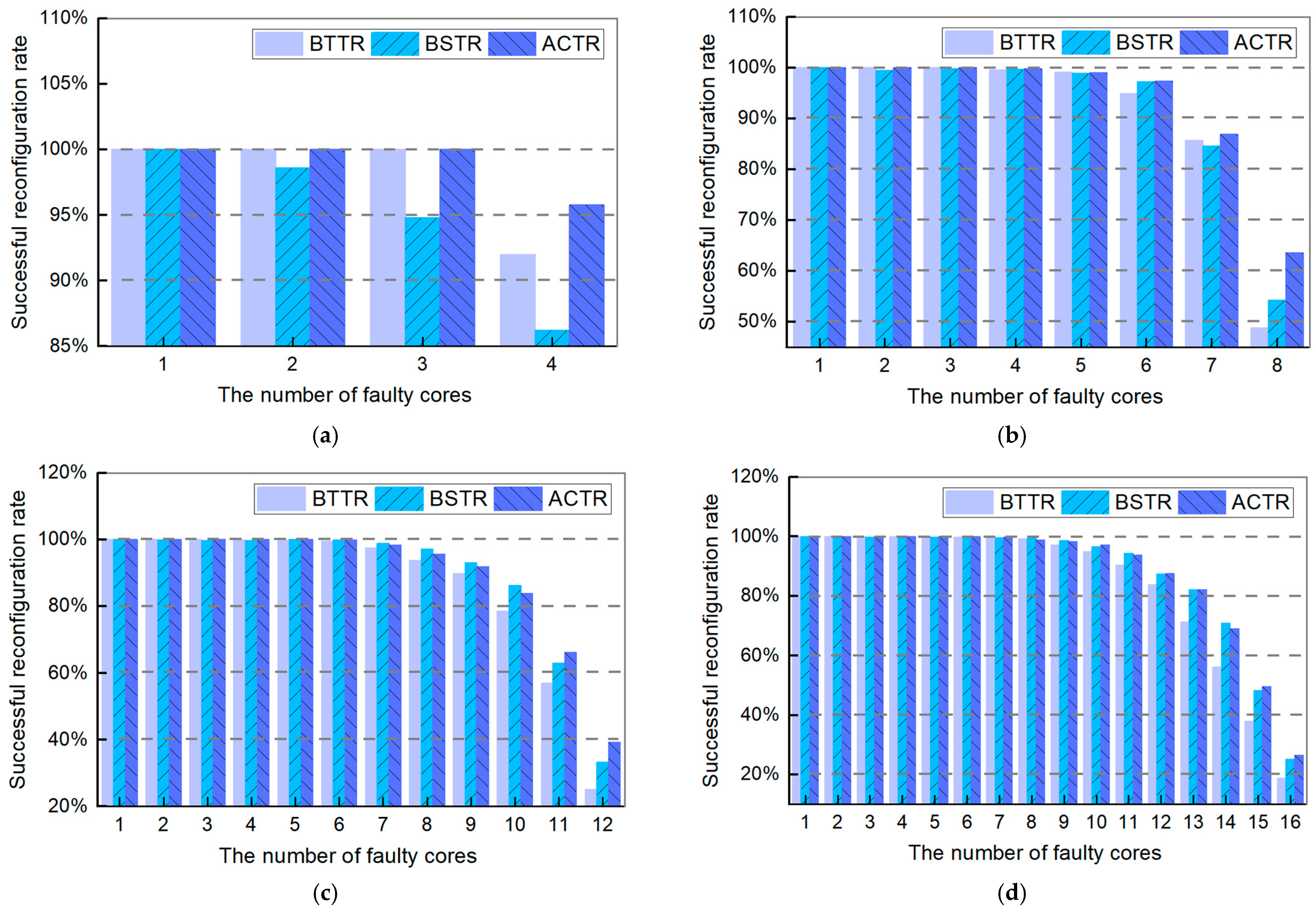
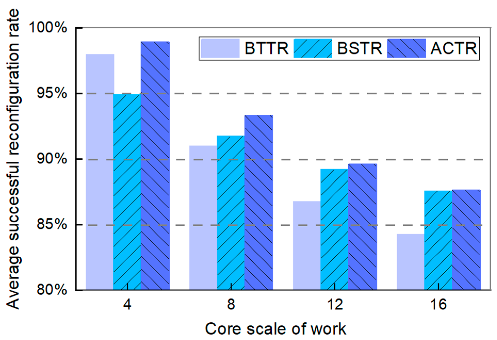
- (1)
- Successful Reconfiguration Rate (SRR)
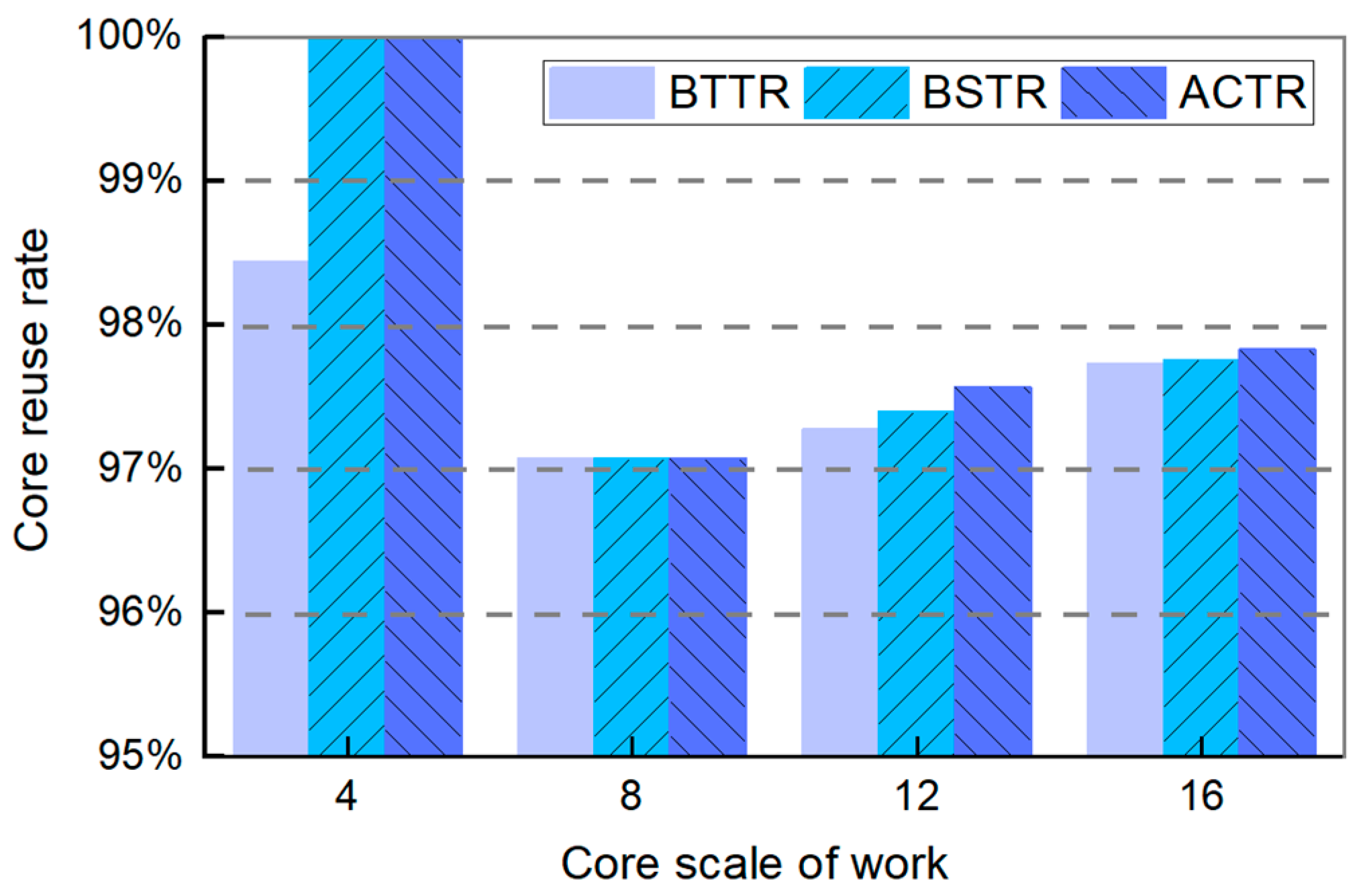
- (2)
- Core Reuse Rate (CRR)
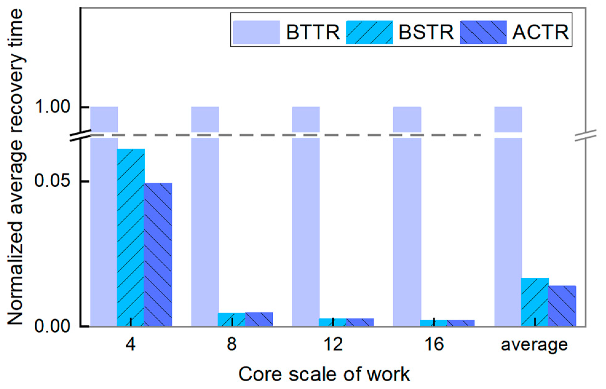
- (3)
- Average Recovery Time (ART)
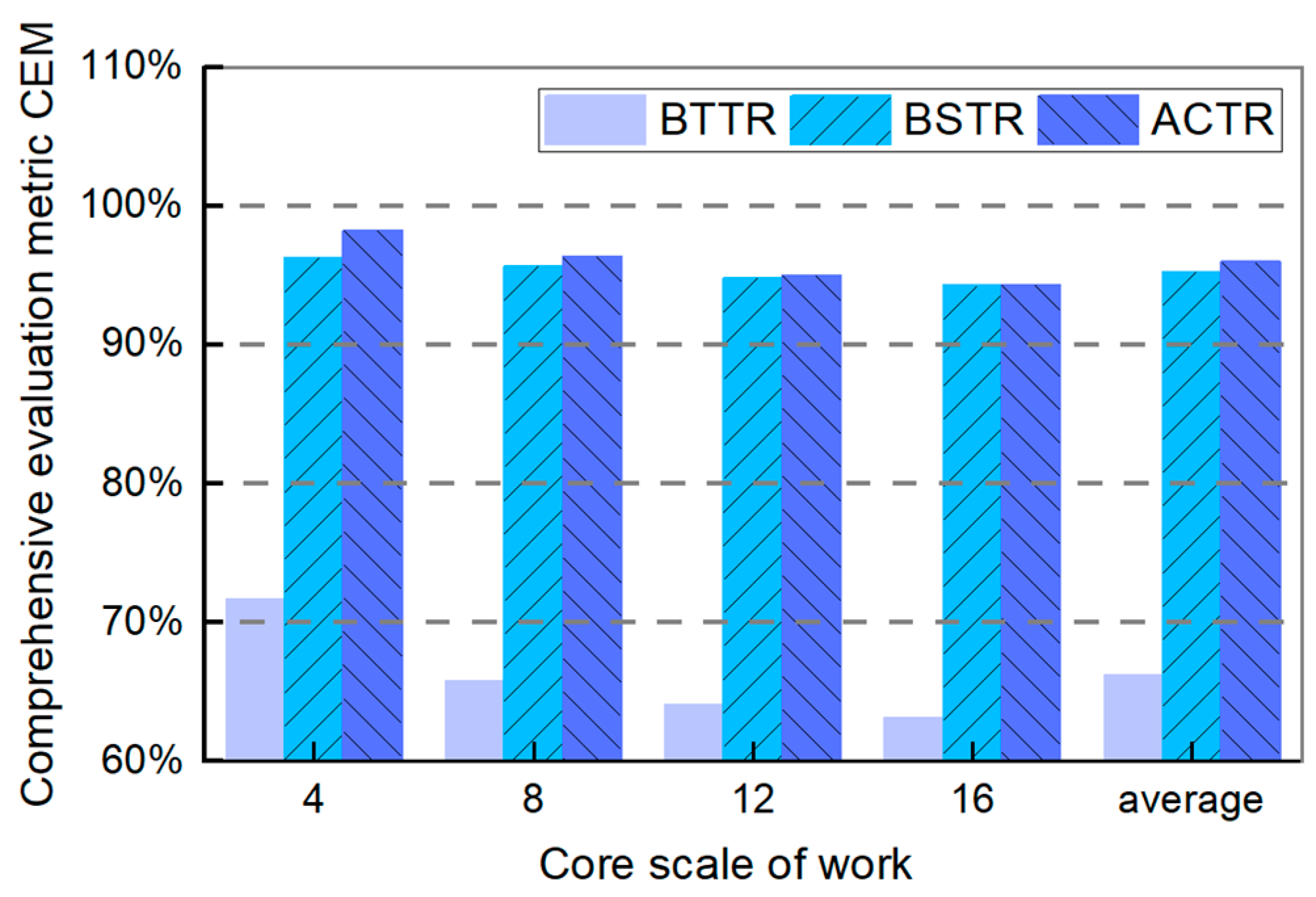
- (4)
- Comprehensive Evaluation Metric (CEM)
7. Conclusions
Author Contributions
Funding
Data Availability Statement
Acknowledgments
Conflicts of Interest
References
- Janac, K.C. Network-on-Chip (NoC): The Technology that Enabled Multi-processor Systems-on-Chip (MPSoCs). In Multi-Processor System-on-Chip 1; ISTE Ltd and John Wiley & Sons, Inc.: London, UK, 2021; pp. 195–225. [Google Scholar]
- Singh, S.; Gupta, V.K.; Mandi, B.C. Leveraging FPGA-based System-on-Chip for Real-time Sensor Data Hosting in IoT. In Proceedings of the 2024 12th International Conference on Internet of Everything, Microwave, Embedded, Communication and Networks (IEMECON), Nagpur, India, 22–23 March 2024; pp. 1–6. [Google Scholar]
- Charles, S.; Mishra, P. A survey of network-on-chip security attacks and countermeasures. ACM Comput. Surv. (CSUR) 2021, 54, 1–36. [Google Scholar]
- Ijaz, Q.; Kidane, H.L.; Bourennane, E.B.; Ochoa-Ruiz, G. Dynamically scalable noc architecture for implementing run-time reconfigurable applications. Micromachines 2023, 14, 1913. [Google Scholar] [CrossRef] [PubMed]
- Zheng, H.; Wang, K.; Louri, A. Adapt-noc: A flexible network-on-chip design for heterogeneous manycore architectures. In Proceedings of the 2021 IEEE international symposium on high-performance computer architecture (HPCA), Virtual Conference, 27 February–3 March 2021; pp. 723–735. [Google Scholar]
- Sarihi, A.; Patooghy, A.; Khalid, A.; Hasanzadeh, M.; Said, M.; Badawy, A.H. A survey on the security of wired, wireless, and 3D network-on-chips. IEEE Access 2021, 9, 107625–107656. [Google Scholar]
- Siddagangappa, R. Asynchronous NoC with Fault tolerant mechanism: A Comprehensive Review. In Proceedings of the 2022 Trends in Electrical, Electronics, Computer Engineering Conference (TEECCON), Shah Alam, Malaysia, 2–4 November 2022; pp. 84–92. [Google Scholar]
- Padmajothi, V.; Iqbal, J.M.; Ponnusamy, V. Load-aware intelligent multiprocessor scheduler for time-critical cyber-physical system applications. Comput. Electr. Eng. 2022, 97, 107613. [Google Scholar]
- Zhu, Y.; Lu, H.; Li, Y.; Zhang, F. Fault-tolerant real-time scheduling algorithm for multicore processors. Electron. Sci. Technol. 2025, 38, 73–80. [Google Scholar] [CrossRef]
- Liu, T.Y. Research on Topology Reconstruction Algorithm for Core-Level Redundancy of Multicore Processors Based on Defect Clustering Effect. Master’s Thesis, Donghua University, Shanghai, China, 2017. [Google Scholar]
- Feng, Y.; Wang, F.; Liu, Z.; Chen, Z. An Online Topology Control Method for Multi-Agent Systems: Distributed Topology Reconfiguration. IEEE Trans. Netw. Sci. Eng. 2024, 11, 4358–4370. [Google Scholar] [CrossRef]
- Romanov, A.; Myachin, N.; Sukhov, A. Fault-tolerant routing in networks-on-chip using self-organizing routing algorithms. In Proceedings of the IECON 2021–47th Annual Conference of the IEEE Industrial Electronics Society, Toronto, Canada, 13–16 October 2021; pp. 1–6. [Google Scholar]
- Yadav, A.K.; Singh, K.M.; Biswas, S. Adaptive BFS based fault tolerant routing algorithm for network on chip. In Proceedings of the 2020 IEEE Region 10 Conference (TENCON), Osaka, Japan, 16–19 November 2020; pp. 170–175. [Google Scholar]
- Nabavi, S.S.; Farbeh, H. A fault-tolerant resource locking protocol for multiprocessor real-time systems. Microelectron. J. 2023, 137, 105809. [Google Scholar] [CrossRef]
- Fasiku, A.I.; Ojedayo, B.O.; Oyinloye, O.E. Effect of routing algorithm on wireless network-on-chip performance. In Proceedings of the 2020 Second International Sustainability and Resilience Conference: Technology and Innovation in Building Designs (51154), Virtual Conference, 11–12 November 2020; pp. 1–5. [Google Scholar]
- Sukhov, A.M.; Romanov, A.Y.; Selin, M.P. Virtual Coordinate System Based on a Circulant Topology for Routing in Networks-On-Chip. Symmetry 2024, 16, 127. [Google Scholar] [CrossRef]
- Luo, R.; Matzner, R.; Zervas, G.; Bayvel, P. Towards a traffic-optimal large-scale optical network topology design. In Proceedings of the 2022 International Conference on Optical Network Design and Modeling (ONDM), Warsaw, Poland, 16–19 May 2022; pp. 1–3. [Google Scholar]
- Li, X.; Yan, G.; Liu, C. Fault-tolerant network-on-chip. In Built-in Fault-Tolerant Computing Paradigm for Resilient Large-Scale Chip Design: A Self-Test, Self-Diagnosis, and Self-Repair-Based Approach; Springer Nature: Singapore, 2023; pp. 169–241. [Google Scholar]
- Bhanu, P.V.; Govindan, R.; Kattamuri, P.; Soumya, J.; Cenkeramaddi, L.R. Flexible spare core placement in torus topology based NoCs and its validation on an FPGA. IEEE Access 2021, 9, 45935–45954. [Google Scholar] [CrossRef]
- Angel, D.; Uma, G.; Priyadharshini, E. Application of Graph theory to Defend Hypercubes and Matching Graph of Hypercube Structures Against Cyber Threats. In Proceedings of the 2023 First International Conference on Advances in Electrical, Electronics and Computational Intelligence (ICAEECI), Tiruchengode, India, 19–20 October 2023; pp. 1–4. [Google Scholar]
- Tie, J.; Pan, G.; Deng, L.; Xun, C.; Luo, L.; Zhou, L. A Method of Extracting and Visualizing Hierarchical Structure of Hardware Logic Based on Tree-Structure For FPGA-Based Prototyping. In Proceedings of the 2024 9th International Symposium on Computer and Information Processing Technology (ISCIPT), Xi’an, China, 24–26 May 2024; pp. 554–561. [Google Scholar]
- Samala, J.; Takawale, H.; Chokhani, Y.; Bhanu, P.V. Fault-tolerant routing algorithm for mesh based NoC using reinforcement learning. In Proceedings of the 2020 24th International Symposium on VLSI Design and Test (VDAT), Virtual Conference, 4–6 July 2020; pp. 1–6. [Google Scholar]
- Zhang, L.; Han, Y.; Li, H.; Li, X. Fault tolerance mechanism in chip many-core processors. Tsinghua Sci. Technol. 2007, 12 (Suppl. S1), 169–174. [Google Scholar]
- Yang, L.; Qin, Z.; Xiao, F.; Wang, S. An optimised topology reconstruction algorithm for core-level redundancy in multicore processors. Comput. Eng. 2015, 41, 50–55. [Google Scholar] [CrossRef]
- Wu, Z.-X. Research on Fault Tolerance Technology of NoC Crowdcore System with Redundant Cores. Ph.D. Thesis, Harbin Institute of Technology, Harbin, China, 2015. [Google Scholar]
- Wu, J.; Wu, Y.; Jiang, G.; Lam, S.K. Algorithms for reconfiguring NoC-based fault-tolerant multiprocessor arrays. J. Circuits Syst. Comput. 2019, 28, 1950111. [Google Scholar] [CrossRef]
- Qian, J.; Zhang, C.; Wu, Z.; Ding, H.; Li, L. Efficient topology reconfiguration for NoC-based multiprocessors: A greedy-memetic algorithm. J. Parallel Distrib. Comput. 2024, 190, 104904. [Google Scholar]
- Zetterstrom, O.; Mesa, F.; Quevedo-Teruel, O. Higher Symmetries in Hexagonal Periodic Structures. In Proceedings of the 2024 18th European Conference on Antennas and Propagation (EuCAP), Glasgow, Scotland, UK, 17–22 March 2024; pp. 1–4. [Google Scholar]
- Romanov, A.Y.; Lezhnev, E.V.; Glukhikh, A.Y.; Amerikanov, A.A. Development of routing algorithms in networks-on-chip based on two-dimensional optimal circulant topologies. Heliyon 2020, 6, e03183. [Google Scholar] [PubMed]
- Bhowmik, B.; Deka, J.K.; Biswas, S. Improving reliability in spidergon network on chip-microprocessors. In Proceedings of the 2020 IEEE 63rd International Midwest Symposium on Circuits and Systems (MWSCAS), Virtual Conference, 9–12 August 2020; pp. 474–477. [Google Scholar]
- Kumar, A.S.; Rao, T.V.K.H. An adaptive core mapping algorithm on NoC for future heterogeneous system-on-chip. Comput. Electr. Eng. 2021, 95, 107441. [Google Scholar] [CrossRef]
- Fu, F.F.; Niu, N.; Xian, X.H.; Wang, J.X.; Lai, F.C. An optimized topology reconfiguration bidirectional searching fault-tolerant algorithm for REmesh network-on-chip. In Proceedings of the 2017 IEEE 12th International Conference on ASIC (ASICON), Guiyang, China, 25–28 October 2017; pp. 303–306. [Google Scholar]
- Niu, N.; Fu, F.F.; Li, H.; Lai, F.C.; Wang, J.X. A Novel Topology Reconfiguration Backtracking Algorithm for 2D REmesh Networks-on-Chip. In Parallel Architecture, Algorithm and Programming: Proceedings of the 8th International Symposium, PAAP 2017, Haikou, China, 17–18 June 2017; Springer: Singapore, 2017; pp. 51–58. [Google Scholar]
- Hu, Y.Y.; Dai, G.Z.; Chen, N.J. Multi-fault tolerant routing algorithm for 2D Mesh. J. Tianjin Polytech. Univ. 2025, 70–76. [Google Scholar]
- Wang, Y.; Yang, X.; Zhuang, H.; Zhu, M.; Kang, L.; Zhao, Y. A resource-optimal logical topology mapping algorithm based on reinforcement learning. Opt. Commun. Technol. 2020, 44, 5. [Google Scholar] [CrossRef]
- Cheng, D.W.; Chang, J.Y.; Lin, C.Y.; Lin, L.; Huang, Y.; Thulasiraman, K.; Hsieh, S.Y. Efficient survivable mapping algorithm for logical topology in IP-over-WDM optical networks against node failure. J. Supercomput. 2023, 79, 5037–5063. [Google Scholar]
- Tomar, D.; Tomar, P.; Bhardwaj, A.; Sinha, G.R. Deep learning neural network prediction system enhanced with best window size in sliding window algorithm for predicting domestic power consumption in a residential building. Comput. Intell. Neurosci. 2022, 2022, 7216959. [Google Scholar] [PubMed]
- Atanda, O.G.; Ismaila, W.; Afolabi, A.O.; Awodoye, O.A.; Falohun, A.S.; Oguntoye, J.P. Statistical Analysis of a deep learning based trimodal biometric system using paired sampling T-Test. In Proceedings of the 2023 International Conference on Science, Engineering and Business for Sustainable Development Goals (SEB-SDG), Omu-Aran, Nigeria, 5–7 April 2023; Volume 1, pp. 1–10. [Google Scholar]
- Tian, Y.; Cao, N. Case Study on the Application of Information Technology in Physical Education Teaching Based on Independent Sample T test. In Proceedings of the 2023 3rd International Conference on Information Technology and Contemporary Sports (TCS), Guangzhou, China, 25–27 August 2022; pp. 6–10. [Google Scholar]
- Yung, Y.K. Enhancing Statistics Education by Choosing the Correct Statistical Tests through a Systematic Approach. In Proceedings of the 2023 11th International Conference on Information and Education Technology (ICIET), Okayama, Japan, 17–19 March 2023; pp. 453–458. [Google Scholar]


| Category | Notations | Description |
|---|---|---|
| Input Parameters | The original physical array | |
| The sliding window used for searching and optimizing | ||
| Set of defect locations in H | ||
| Dimensions and number of faulty elements | ||
| Output Parameters | Final target array that is optimized |
Disclaimer/Publisher’s Note: The statements, opinions and data contained in all publications are solely those of the individual author(s) and contributor(s) and not of MDPI and/or the editor(s). MDPI and/or the editor(s) disclaim responsibility for any injury to people or property resulting from any ideas, methods, instructions or products referred to in the content. |
© 2025 by the authors. Licensee MDPI, Basel, Switzerland. This article is an open access article distributed under the terms and conditions of the Creative Commons Attribution (CC BY) license (https://creativecommons.org/licenses/by/4.0/).
Share and Cite
Hou, B.; Xu, D.; Fu, F.; Yang, B.; Niu, N. An Optimized Core Distribution Adaptive Topology Reconfiguration Algorithm for NoC-Based Embedded Systems. Micromachines 2025, 16, 421. https://doi.org/10.3390/mi16040421
Hou B, Xu D, Fu F, Yang B, Niu N. An Optimized Core Distribution Adaptive Topology Reconfiguration Algorithm for NoC-Based Embedded Systems. Micromachines. 2025; 16(4):421. https://doi.org/10.3390/mi16040421
Chicago/Turabian StyleHou, Bowen, Dali Xu, Fangfa Fu, Bing Yang, and Na Niu. 2025. "An Optimized Core Distribution Adaptive Topology Reconfiguration Algorithm for NoC-Based Embedded Systems" Micromachines 16, no. 4: 421. https://doi.org/10.3390/mi16040421
APA StyleHou, B., Xu, D., Fu, F., Yang, B., & Niu, N. (2025). An Optimized Core Distribution Adaptive Topology Reconfiguration Algorithm for NoC-Based Embedded Systems. Micromachines, 16(4), 421. https://doi.org/10.3390/mi16040421