
Super-Resolution Reconstruction of Cytoskeleton Image Based on A-Net Deep Learning Network


Abstract
:1. Introduction
2. Related Works
2.1. Traditional Methods
2.2. Deep-Learning-Based Algorithm
3. Algorithm
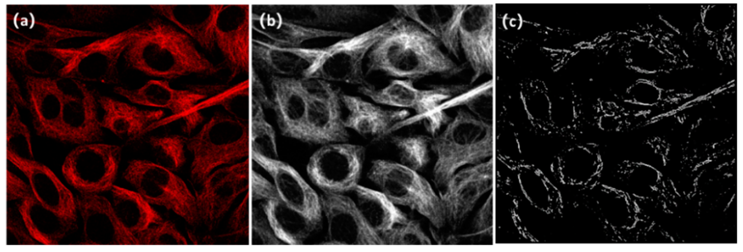
3.1. Raw Images and Processing Targets
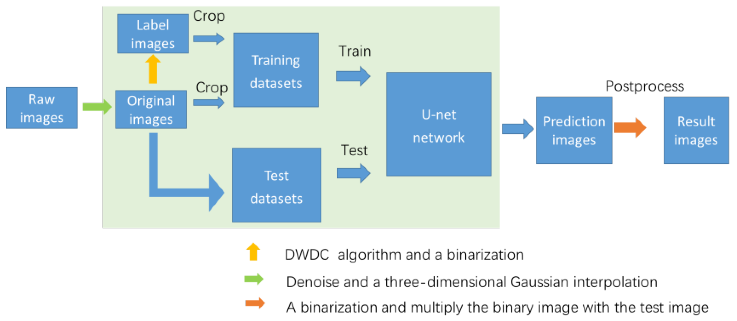
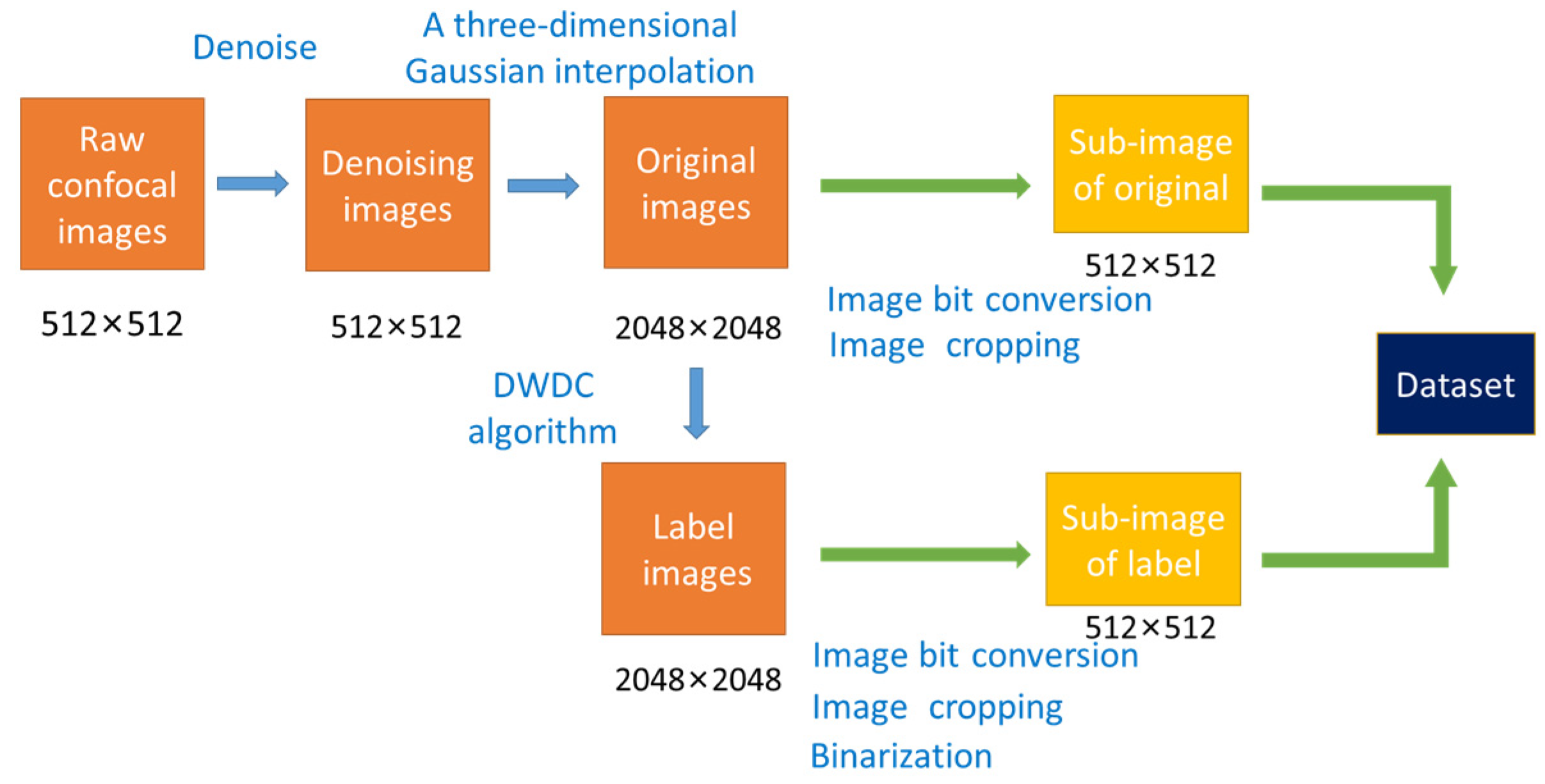
3.2. Preprocessing
3.3. A-Net Network
3.4. Postprocessing
4. Experiments
4.1. SR_MUI Dataset
4.2. Implementation
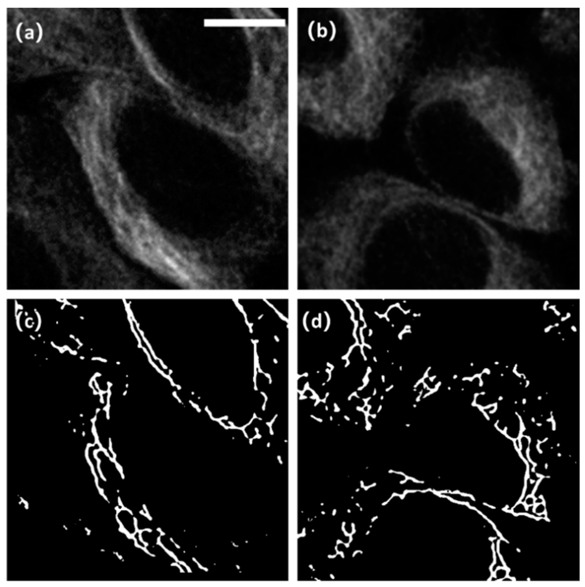
5. Results
6. Conclusions
Author Contributions
Funding
Institutional Review Board Statement
Informed Consent Statement
Data Availability Statement
Acknowledgments
Conflicts of Interest
References
- Kim, Y.; Cha, M.; Choi, Y.; Joo, H.; Lee, J. Electrokinetic separation of biomolecules through multiple nano-pores on membrane. Chem. Phys. Lett. 2013, 561, 63–67. [Google Scholar] [CrossRef]
- Furuya, K.; Sokabe, M.; Furuya, S. Characteristics of subepithelial fibroblasts as a mechano-sensor in the intestine: Cell-shape-dependent ATP release and P2Y1 signaling. J. Cell Sci. 2005, 118, 3289–3304. [Google Scholar] [CrossRef]
- Hays, J.B.; Magar, M.E.; Zimm, B.H. Persistence length of DNA. Biopolym. Orig. Res. Biomol. 1969, 8, 531–536. [Google Scholar] [CrossRef]
- Friede, R.L.; Samorajski, T. Axon caliber related to neurofilaments and microtubules in sciatic nerve fibers of rats and mice. Anat. Rec. 1970, 167, 379–387. [Google Scholar] [CrossRef] [PubMed]
- Williams, D.B.; Carter, C.B. The transmission electron microscope. In Transmission Electron Microscopy; Springer: Boston, MA, USA, 1996; pp. 3–17. [Google Scholar]
- Crewe, A.V.; Isaacson, M.; Johnson, D. A simple scanning electron microscope. Rev. Sci. Instrum. 1969, 40, 241–246. [Google Scholar] [CrossRef]
- Adrian, M.; Dubochet, J.; Lepault, J.; McDowall, A.W. Cryo-electron microscopy of viruses. Nat. Methods 1984, 308, 32–36. [Google Scholar] [CrossRef] [PubMed]
- Vicidomini, G.; Bianchini, P.; Diaspro, A. STED super-resolved microscopy. Nat. Methods 2018, 15, 173. [Google Scholar] [CrossRef]
- Timpson, P.; McGhee, E.J.; Anderson, K.I. Imaging molecular dynamics in vivo—From cell biology to animal models. J. Cell Sci. 2011, 124, 2877–2890. [Google Scholar] [CrossRef]
- Radtke, S.; Adair, J.E.; Giese, M.A.; Chan, Y.-Y.; Norgaard, Z.K.; Enstrom, M.; Haworth, K.G.; Schefter, L.E.; Kiem, H.-P. A distinct hematopoietic stem cell population for rapid multilineage engraftment in nonhuman primates. Sci. Transl. Med. 2017, 9, eaan1145. [Google Scholar] [CrossRef]
- Davila, J.C.; Cezar, G.G.; Thiede, M.; Strom, S.; Miki, T.; Trosko, J. Use and application of stem cells in toxicology. Toxicol. Sci. 2004, 79, 214–223. [Google Scholar] [CrossRef] [Green Version]
- Sousa, A.A.; Leapman, R.D. Development and application of STEM for the biological sciences. Ultramicroscopy 2012, 123, 38–49. [Google Scholar] [CrossRef]
- Lu, X.; Wang, Y.; Fung, S.; Qing, X. I-Nema: A Biological Image Dataset for Nematode Recognition. arXiv 2021, arXiv:2103.08335. [Google Scholar]
- Hunt, B.R. Super-resolution of images: Algorithms, principles, performance. Int. J. Imaging Syst. Technol. 1995, 6, 297–304. [Google Scholar] [CrossRef]
- Ng, M.K.; Bose, N.K. Mathematical analysis of super-resolution methodology. IEEE Signal Processing Mag. 2003, 20, 62–74. [Google Scholar] [CrossRef]
- Dong, C.; Loy, C.C.; He, K.; Tang, X. Learning a deep convolutional network for image super-resolution. In European Conference on Computer Vision; Springer: Cham, Switzerland, 2014. [Google Scholar]
- Dong, C.; Loy, C.C.; Tang, X. Accelerating the super-resolution convolutional neural network. In European Conference on Computer Vision; Springer: Cham, Switzerland, 2016. [Google Scholar]
- Ledig, C.; Theis, L.; Huszár, F.; Caballero, J.; Cunningham, A.; Acosta, A.; Aitken, A.; Tejani, A.; Totz, J.; Wang, Z. Photo-Realistic Single Image Super-Resolution Using a Generative Adversarial Network. In Proceedings of the IEEE Conference on Computer Vision and Pattern Recognition, Honolulu, HI, USA, 21–26 July 2017. [Google Scholar]
- Bai, H.; Bingchen, C.; Zhao, T.; Zhao, W.; Wang, K.; Zhang, C.; Bai, J. Bioimage postprocessing based on discrete wavelet transform and Lucy-Richardson deconvolution (DWDC) methods. bioRxiv 2021. [Google Scholar] [CrossRef]
- Hojjatoleslami, S.A.; Avanaki, M.R.N.; Podoleanu, A. Gh Image quality improvement in optical coherence tomography using Lucy–Richardson deconvolution algorithm. Appl. Opt. 2013, 52, 5663–5670. [Google Scholar] [CrossRef]
- Devi, A.G.; Madhum, T.; Kishore, K.L. A Novel Super Resolution Algorithm based on Fuzzy Bicubic Interpolation Algorithm. Int. J. Signal Processing Image Processing Pattern Recognit. 2015, 8, 283–298. [Google Scholar] [CrossRef]
- Zhang, Y.; Fan, Q.; Bao, F.; Liu, Y.; Zhang, C. Single-Image Super-Resolution Based on Rational Fractal Interpolation. IEEE Trans. Image Processing 2018, 27, 3782–3797. [Google Scholar]
- Tao, H.; Tang, X. Superresolution remote sensing image processing algorithm based on wavelet transform and interpolation. Image Processing Pattern Recognit. Remote Sens. 2003, 4898, 259–263. [Google Scholar]
- Nitta, K.; Shogenji, R.; Miyatake, S.; Tanida, J. Image reconstruction for thin observation module by bound optics by using the iterative backprojection method. Appl. Opt. 2006, 45, 2893–2900. [Google Scholar] [CrossRef]
- Fan, C.; Wu, C.; Li, G.; Ma, J. Projections onto Convex Sets Super-Resolution Reconstruction Based on Point Spread Function Estimation of Low-Resolution Remote Sensing Images. Sensors 2017, 17, 362. [Google Scholar] [CrossRef] [PubMed]
- Wang, L.-G.; Zhao, Y. MAP based super-resolution method for hyperspectral imagery. Guang Pu Xue Yu Guang Pu Fen Xi=Guang Pu 2010, 30, 1044–1048. [Google Scholar] [PubMed]
- Huang, D.; Huang, W.; Yuan, Z.; Lin, Y.; Zhang, J.; Zheng, L. Image Super-Resolution Algorithm Based on an Improved Sparse Autoencoder. Information 2018, 9, 11. [Google Scholar] [CrossRef] [Green Version]
- Lin, Z.; He, J.; Tang, X.; Tang, C.K. Limits of Learning-Based Superresolution Algorithms. Int. J. Comput. Vis. 2008, 80, 406–420. [Google Scholar] [CrossRef]
- Rajaram, S.; Gupta, M.D.; Petrovic, N.; Huang, T.S. Learning-Based Nonparametric Image Super-Resolution. EURASIP J. Adv. Signal Processing 2006, 2006, 51306. [Google Scholar] [CrossRef]
- Li, X.; Wu, Y.; Zhang, W.; Wang, R.; Hou, F. Deep learning methods in real-time image super-resolution: A survey. J. Real-Time Image Processing 2019, 17, 1885–1909. [Google Scholar] [CrossRef]
- Sanchez-Beato, A.; Pajares, G. Noniterative Interpolation-Based Super-Resolution Minimizing Aliasing in the Reconstructed Image. IEEE Trans. Image Processing 2008, 17, 1817–1826. [Google Scholar] [CrossRef]
- Zhou, F.; Yang, W.; Liao, Q. Interpolation-Based Image Super-Resolution Using Multisurface Fitting. IEEE Trans. Image Processing 2012, 21, 3312–3318. [Google Scholar] [CrossRef]
- Zomet, A.; Rav-Acha, A.; Peleg, S. Robust super-resolution. In Proceedings of the 2001 IEEE Computer Society Conference on Computer Vision and Pattern Recognition, CVPR 2001, Kauai, HI, USA, 8–14 December 2001. [Google Scholar]
- Patel, V.; Modi, C.K.; Paunwala, C.N.; Patnaik, S. Hybrid Approach for Single Image Super Resolution Using ISEF and IBP. In Proceedings of the 2011 International Conference on Communication Systems and Network Technologies, Katra, India, 3–5 June 2011. [Google Scholar]
- Lukeš, T.; Křížek, P.; Švindrych, Z.; Benda, J.; Ovesný, M.; Fliegel, K.; Klíma, M.; Hagen, G.M. Three-dimensional super-resolution structured illumination microscopy with maximum a posteriori probability image estimation. Opt. Express 2014, 22, 29805–29817. [Google Scholar] [CrossRef]
- Babacan, S.D.; Molina, R.; Katsaggelos, A.K. Variational Bayesian super resolution. IEEE Trans. Image Processing 2010, 20, 984–999. [Google Scholar] [CrossRef]
- Humblot, F.; Mohammad-Djafari, A. Super-resolution Using Hidden Markov Model and Bayesian Detection Estimation Framework. EURASIP J. Adv. Signal Processing 2006, 2006, 126–141. [Google Scholar] [CrossRef]
- Wu, W.; Liu, Z.; He, X. Learning-based super resolution using kernel partial least squares. Image Vis. Comput. 2011, 29, 394–406. [Google Scholar] [CrossRef]
- Gajjar, P.P.; Joshi, M.V. New learning based super-resolution: Use of DWT and IGMRF prior. IEEE Trans. Image Processing 2010, 19, 1201–1213. [Google Scholar] [CrossRef]
- Bevilacqua, M.; Roumy, A.; Guillemot, C.; Alberi-Morel, M.L. Low-complexity single-image super-resolution based on nonnegative neighbor embedding. In Proceedings of the British Machine Vision Conference, Guildford, UK, 3–7 September 2012; pp. 135.1–135.10. [Google Scholar]
- Zhang, Y.; Du, Y.; Ling, F.; Fang, S.; Li, X. Example-Based Super-Resolution Land Cover Mapping Using Support Vector Regression. IEEE J. Sel. Top. Appl. Earth Obs. Remote Sens. 2014, 7, 1271–1283. [Google Scholar] [CrossRef]
- Ni, K.S.; Nguyen, T.Q. Image Superresolution Using Support Vector Regression. IEEE Trans. Image Processing 2007, 16, 1596–1610. [Google Scholar] [CrossRef]
- Lu, X.; Yuan, Y.; Yan, P. Image Super-Resolution Via Double Sparsity Regularized Manifold Learning. IEEE Trans. Circuits Syst. Video Technol. 2013, 23, 2022–2033. [Google Scholar] [CrossRef]
- Yang, J.; Wright, J.; Huang, T.S.; Ma, Y. Image Super-Resolution Via Sparse Representation. IEEE Trans. Image Processing 2010, 19, 2861–2873. [Google Scholar] [CrossRef]
- Zhu, Z.; Guo, F.; Yu, H.; Chen, C. Fast Single Image Super-Resolution via Self-Example Learning and Sparse Representation. IEEE Trans. Multimed. 2014, 16, 2178–2190. [Google Scholar] [CrossRef]
- Kim, J.; Kwon, L.J.; Mu, L.K. Accurate Image Super-resolution Using Very Deep Nonvolutional Networks. In Proceedings of the 2016 IEEE Conference on Computer Vision and Pattern Recognition (CVPR), Las Vegas, NV, USA, 27–30 June 2016; pp. 1646–1654. [Google Scholar]
- Ronneberger, O.; Fischer, P.; Brox, T. U-Net: Convolutional Networks for Biomedical Image Segmentation. In International Conference on Medical Image Computing and Computer-Assisted Intervention; Springer: Cham, Switzerland, 2015. [Google Scholar]
- Vicidomini, G.; Hell, S.W.; Schönle, A. Automatic deconvolution of 4Pi-microscopy data with arbitrary phase. Opt. Lett. 2009, 34, 3583–3585. [Google Scholar] [CrossRef]
- Liu, Y.; Lu, Y.; Yang, X.; Zheng, X.; Wen, S.; Wang, F.; Vidal, X.; Zhao, J.; Liu, D.; Zhou, Z.; et al. Amplified stimulated emission in upconversion nanoparticles for super-resolution nanoscopy. Nature 2017, 543, 229–233. [Google Scholar] [CrossRef]
- Westphal, V.; Rizzoli, S.O.; Lauterbach, M.A.; Kamin, D.; Jahn, R.; Hell, S.W. Video-Rate Far-Field Optical Nanoscopy Dissects Synaptic Vesicle Movement. Science 2008, 320, 246–249. [Google Scholar] [CrossRef] [PubMed] [Green Version]


Publisher’s Note: MDPI stays neutral with regard to jurisdictional claims in published maps and institutional affiliations. |
© 2022 by the authors. Licensee MDPI, Basel, Switzerland. This article is an open access article distributed under the terms and conditions of the Creative Commons Attribution (CC BY) license (https://creativecommons.org/licenses/by/4.0/).
Share and Cite
Chen, Q.; Bai, H.; Che, B.; Zhao, T.; Zhang, C.; Wang, K.; Bai, J.; Zhao, W. Super-Resolution Reconstruction of Cytoskeleton Image Based on A-Net Deep Learning Network. Micromachines 2022, 13, 1515. https://doi.org/10.3390/mi13091515
Chen Q, Bai H, Che B, Zhao T, Zhang C, Wang K, Bai J, Zhao W. Super-Resolution Reconstruction of Cytoskeleton Image Based on A-Net Deep Learning Network. Micromachines. 2022; 13(9):1515. https://doi.org/10.3390/mi13091515
Chicago/Turabian StyleChen, Qian, Haoxin Bai, Bingchen Che, Tianyun Zhao, Ce Zhang, Kaige Wang, Jintao Bai, and Wei Zhao. 2022. "Super-Resolution Reconstruction of Cytoskeleton Image Based on A-Net Deep Learning Network" Micromachines 13, no. 9: 1515. https://doi.org/10.3390/mi13091515
APA StyleChen, Q., Bai, H., Che, B., Zhao, T., Zhang, C., Wang, K., Bai, J., & Zhao, W. (2022). Super-Resolution Reconstruction of Cytoskeleton Image Based on A-Net Deep Learning Network. Micromachines, 13(9), 1515. https://doi.org/10.3390/mi13091515