1. Introduction
Blood is a multi-component suspension and consists mostly of plasma (~55%), red blood cells (RBCs, ~45%) and white blood cells and platelets (~1%). Due to their high content, RBCs play major role in flow dynamics and rheological properties of blood. A healthy RBC has a biconcave shape with a diameter 6–8
m and thickness 2
m [
1]. The RBC membrane consists of a lipid bilayer and a spectrin network attached to the inner side of the bilayer. The cytoplasm contains mostly hemoglobin, a protein responsible for oxygen transfer. This protein causes higher viscosity of the inner cytoplasm compared to the outer plasma, which is referred to as viscosity contrast.
The blood flow in large vessels is mostly driven by a uniform shear flow that occurs near the vessel walls or by the fairly uniform flow in the central parts of the vessels. On the contrary, in vessel bifurcations and in small arterioles and microcapilaries with diameters comparable to the size of the cells, the parabolic velocity profile introduces non-uniformity and the flow patterns differ significantly from those in large vessels.
The shape of the red blood cell in large vessels is mostly close to the relaxed biconcave shape or to prolonged ellipsoidal shapes, with dynamic patterns such as tumbling and tank-treading [
2,
3,
4,
5]. In capillaries, the shape patterns are richer. Different flow conditions result in cup-like parachute shapes at the vessel center, elongated slipper shapes at an off-center position, bullet-like shapes in very narrow vessels, snaking dynamics—a periodic cell swinging around the tube center, or tumbling trilobe state at large flow rates and low confinements [
6].
Besides the flow conditions and the elasticity of the membrane, an important parameter influencing the cell dynamics is the viscosity contrast
. It has been shown that
significantly affects the RBC behavior in simple shear flow [
7,
8,
9,
10]. Only recently, several studies have confirmed that the viscosity contrast is important in microcapillary flow [
6,
11,
12,
13,
14]. In [
6], the authors study the dependence of the RBC shape and dynamics on the viscosity contrast in tube flow. They provide state diagrams of RBC dynamical states for various viscosity contrasts and wide ranges of flow rates and tube diameters. They conclude that the region of parachute shapes is significantly larger for
in comparison to
. In another study [
13], many-cell simulations show an increasing difference between relative apparent viscosity for
and
with increasing Reynolds number. This indicates that the viscosity contrast plays a more important role as the flow shear rates increase.
An interesting result concerns the cell free layer (CFL). While in works [
11,
13] the authors conclude that the viscosity contrast influences the thickness of the CFL only very weakly, if at all, the opposite conclusion has been drawn in [
14] where the authors claim that at 10% hematocrit, the viscosity contrast is not negligible when calculating the CFL thickness. They study small arteriole flows (20–40
m) with a hematocrit of 10–20% and a physiological viscosity contrast, which is
on average [
15,
16].
The viscosity contrast has proven to play an important role in microcirculation. In this work, we employ a novel approach to taking the viscosity contrast into account. We extend the existing red blood cell model based on lattice-Botzmann method (LBM) for governing the fluid and spring network for governing the elasticity of cell membrane [
17,
18]. We include dissipative particles (DPs) inside the cell as a coarse-grained hemoglobin model to increase the viscosity of the resulting suspension inside the cell. We analyse the influence of suspension properties on its effective viscosity. We model two scenarios to measure the suspension viscosity. The results from these two computational experiments are then used in the RBC model with DPs. The new model is validated using biological data from the static RBC stretching and the dynamic release [
19].
2. Viscosity Contrast in Other Red Blood Cell Models
Many of the recent simulation studies for simplicity assume the viscosity contrast
[
20,
21,
22,
23]. For lower shear stresses and for the flows with no small confinements, it is a reasonable assumption that can be deduced from conclusions of [
11,
13].
There are, however, models that assume non-unit viscosity contrast. The continuous model in [
14] for example treats the coupled problem governed by Navier–Stokes equations that conserve momentum both in the fluid and in the membrane sub-domains. Computational domain is divided into fluid and cell with the stress balance to be satisfied at the boundary of fluid and cell. The cell is modeled as a 2D hyperelastic membrane with Skalak model. To solve the coupled fluid–solid problem, they utilize an Immersed Finite Element Method. The viscosity contrast is naturally incorporated by different fluid properties inside the cell domain. This method requires re-meshing of the computational domain when the cell deforms.
The method in [
6,
11] is based on smoothed dissipative particle dynamics. Here, the fluid consists of fluid particles which interact through conservative, dissipative and random forces. The cytosol inside the RBC is separated from the outside fluid (plasma) by the layer of membrane particles. The number of membrane particles is typically around 3000 and the density of the fluid particles can be set from 9 to 12 per unit volume (1
m
) [
6,
11]. The viscosity of the inner and outer fluid is achieved by frictional dissipative force between neighbouring particles. Therefore, the viscosity contrast can be increased simply by taking two different magnitudes of the dissipative forces for the inner and outer particles. The elasticity of the membrane is achieved by using a spring network of particles with elastic moduli: stretching, bending, local and global area and volume modulus. The elastic forces are computed by minimization of total potential energy of the particle system.
The model in [
13] consists of coupled lattice-Boltzmann and Immersed Boundary method (IBM). The blood plasma is represented as a continuous incompressible Newtonian fluid that is computed using LBM with a fixed lattice with 19 directions providing second order accuracy for fluid computations. The cells are represented as spring-network meshes with elastic properties defined by the total potential energy similar to that of the model presented in [
6,
11]. The fluid and the membrane are coupled using a validated immersed boundary method [
22]. The fluid viscosity in LBM is controlled by a relaxation parameter
and in general, this parameter can be variable in space ensuring different viscosities at different locations. It is important to carefully handle the discontinuity when considering two distinct viscosities for inner and outer membrane fluid. To introduce a viscosity contrast into such model, one needs to keep track of the fluid nodes residing inside the RBC membranes. These membranes are represented as closed surface triangular meshes which enclose lattice nodes of the fluid grid. For these grid nodes, the relaxation parameter
of the LBM method can be altered to express the increase in local viscosity. In [
22], determining whether a lattice point is inside an RBC was done using the ray-casting algorithm, where for a point inside or outside a polygon a ray is cast and the number of membrane intersections is counted. Odd number means the point is an interior point. Although the complexity of such algorithm is high, the authors have optimised the performance to ensure the increase in typical runtime is less than 25%.
3. RBC Model and the Concept of Dissipative Particles
We work with an RBC model that we previously developed and introduced in [
17,
18]. The model consists of two principal components: the fluid and elastic objects immersed in it. For the fluid, we use the lattice-Boltzmann method [
24]. The three-dimensional space is discretized with a fixed lattice. Fictive particles can move and collide over the edges and the diagonals of this lattice, representing coarse-grained fluid. From the density and movements of these particles, one can express the velocity, density and other properties of the fluid in each time step on a fixed lattice grid.
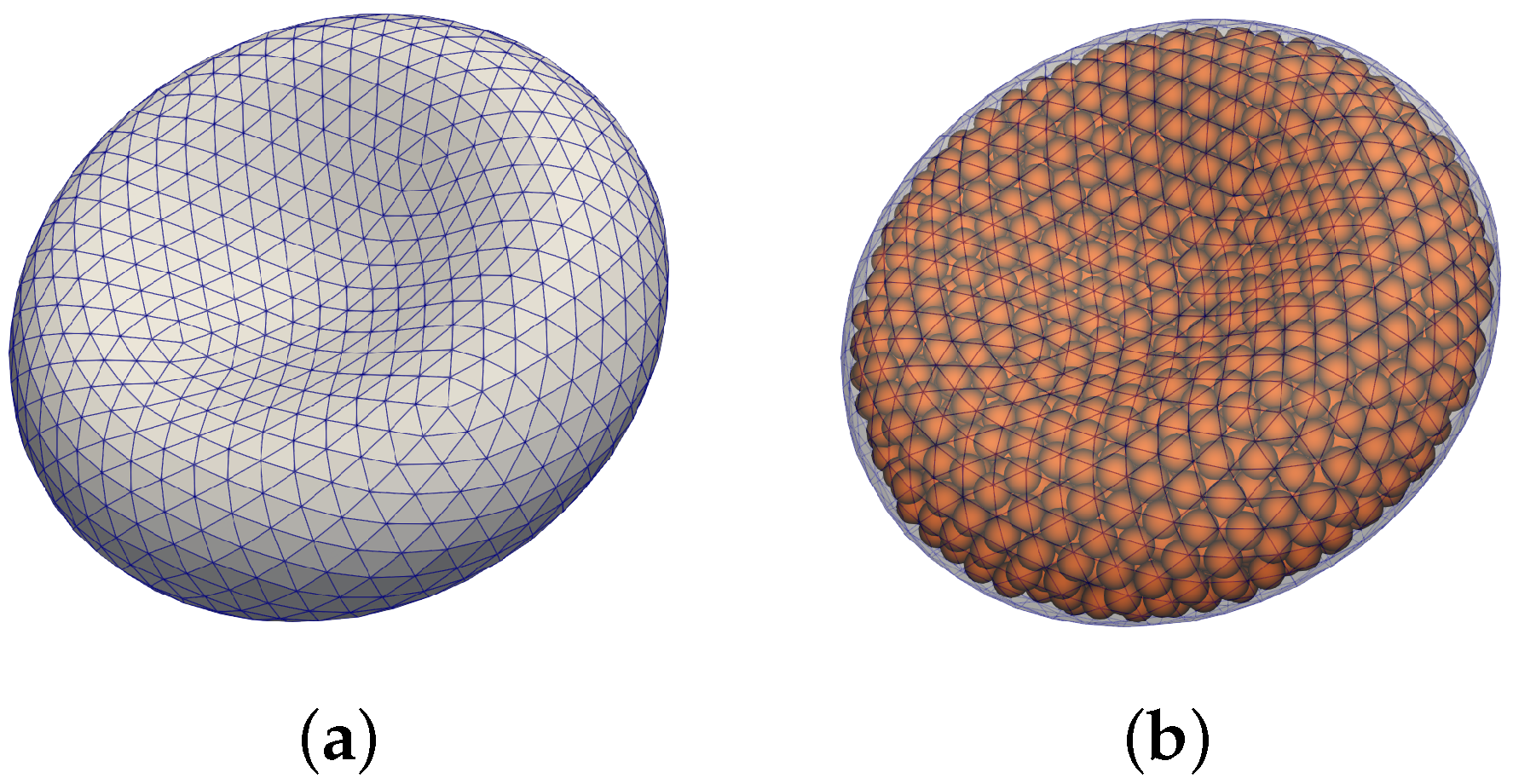
The second component is a triangular mesh representing a closed surface of the cell membrane, see
Figure 1a. The elastic properties of the object are represented with different types of force-like bonds between neighboring mesh points. This way, the deformation of the object changes the relaxed distances between the mesh points and this induces forces acting against the change at the corresponding mesh points.
Unlike in the IBM described above, the fluid and the elastic objects are coupled via a dissipative force here. Forces induced by the cell deformation enter the lattice-Boltzmann equation. Analogously, fluid forces are also transferred to the object’s mesh points. This method has been known as Immersed Boundary via Dissipative Coupling (IB-DC).
The two distinct meshes—the lattice mesh for the fluid and the triangular mesh for the cell—overlap, which results in uniform viscosity for the fluid inside and outside the cell. One solution for introducing the viscosity contrast in LBM was described above in combination with the IBM method [
13]. Another solution, presented here, is to introduce the viscosity contrast by mimicking the biological essence of cytosol content, the hemoglobin proteins.
The major component of RBC is water (721 mg mL
RBC), which is twice the mass of total RBC protein (371 mg mL
RBC). Hemoglobin makes up 95% of total RBC protein [
25]. This may suggest that including hemoglobin into the model of RBC would lead to correct modelling of the viscosity contrast.
Hemoglobin is a protein that folds into globular structures [
26]. There are no substantial holes and almost no water molecules in the protein interior. As a consequence, the proteins are rigid structures. Their spheroidal shape was confirmed by micrograph [
27] to be of 6 × 6 × 5 nm
as presented in Table 4 in [
28].
In this work, we employ a coarse-graining method called dissipative particle dynamics (DPD). Since modelling each individual hemoglobin molecule is computationally too expensive (rough calculation would lead to
hemoglobin molecules in one cell), we represent a virtual cluster of hemoglobin molecules as one soft dissipative particle (DP). The dissipative forces are included in the particle interactions due to the eliminated degree of freedom during the coarse-graining procedure [
29]. Similar approach for modelling of the aligned hemoglobin polymer in sickle-cell RBCs was presented in [
30,
31]. The vizualization of the model with particles is depicted in
Figure 1b.
4. Practical Considerations for Model Implementation
The typical number of mesh points in the triangular mesh of IB-DC model can vary. At least 200 mesh points are needed to capture the cell shape properly but with increased demand on the accuracy, the mesh can contain up to few thousand mesh-points. The aim is to keep the complexity of the model comparable and thus the number of inner particles should not exceed couple thousand.
The coarse-graining procedure clusters a large number of hemoglobin molecules into one dissipative particle. Although the hemoglobin molecules are rigid, the virtual clustering causes the particle to be soft. It is thus modelled as a non-dimensional particle with radius interacting with other particles by two kinds of forces: conservative and dissipative. The classical DPD approach also includes random forces but on the scale we are interested in, the Brownian motion is not of the interest and thus we omit the random component. The conservative forces depend on the position of the particles and are purely repulsive, while the dissipative forces depend on the relative velocity between the particles.
Conservative forces We consider two different repulsive potentials with cutoff distance being twice the radius of the DPs.
The first is the soft-sphere potential leading to the repulsive forces
between two particles at distance
d
where the parameters
define the magnitude and steepness of the potential and
its cutoff distance. Note that the soft-sphere forces blow up at zero particle distance and are not continuous at the cutoff distance.
The second potential is a hat potential defined as
where
defines the maximal repulsive force when the two particles overlap which linearly decreases to zero at cutoff distance
.
Dissipative forces For modelling of the viscosity, the dissipative forces consist of two components, one that aligns with the particle-particle line and one that is perpendicular to it:
where
denotes scalar product,
is the unit vector between two particles
,
is the relative velocity and
is the cutoff radius. Although the dissipative forces have two distinct contributions, parallel with and normal to
and can in principle be scaled differently, we use a common multiplicative parameter
for both of them, so
The number of particles inside an RBC can vary and depends on the and the desired solid-volume fraction . Both and influence the viscosity of the resulting suspension.
To ensure that the DPs stay within the cell membrane, we use another soft-sphere potential defining the repulsive forces
between the membrane mesh and the DPs. The definition of
is analogous to
with parameters
and
. The cutoff radius for this potential is denoted by
and its fine-tuning depends on the size of edges in the triangular membrane mesh. The cutoff radius
must be large enough so that the DPs cannot slip through any of the triangles. A reasonable value of
is the average length of the edges in the relaxed mesh. A similar force is also used for the repulsive interaction between the membrane and the outer suspension in
Section 5.2.2 with parameters given in
Table A4.
Once we decide the size and number of particles, we randomly seed them inside a rhomboid inscribed into the cell. We turn on the repulsive forces between the DPs and between the DPs and the triangular mesh and we let the particles relax into equilibrium. An increase in or is needed if they do not fill up the whole inner region of the cell. The resulting equilibrium positions are saved and used later for subsequent simulations as initial seedings.
5. Viscosity of Particle Suspensions
Particles suspended in liquid increase its effective viscosity. There are different phenomena for suspensions of rigid particles and soft particles.
5.1. Suspensions of Spheres or Colloids
For rigid spheres, it is possible to derive analytical formulas that relate the viscosity of suspension to the underlying solid volume fraction. If the particle concentration
is very low (≲0.1 volume fraction), the resulting viscosity can be expressed as
where
is the viscosity of the underlying fluid [
32]. The corrected version for a dilute emulsion of viscous droplets was derived in [
33]
where
is the viscosity of the droplet fluid.
The Formula (
1) was later adapted [
34,
35] in the case of pure straining without effect of Brownian motion for spheres of the same size with total volume fraction from 0.15 to 0.2 as
For even higher volume fractions there is an analytical expression [
36] that takes into account also two other parameters
where
is the maximum possible solid fraction and
is a parameter related to particle shape (with value of 2.5 for spheres). The maximum solid fraction is
for a regular packing and approximately
for a random packing of spheres [
37].
While the formulas for rigid spheres are not easily applied to soft-sphere suspensions that exhibit much richer rheological properties, they can serve as an upper bound.
For colloidal suspensions [
38,
39], the models treat particles as hard or soft spheres with lubrication forces suspended in a fluid. The modelling of particle behaviour involves tracking their position, mass and rotational inertia that enter the Newton motion equations together with lubrication forces. The results presented in the above works show nonlinear dependence of the suspension viscosity on the volume fraction and the shear rate.
In Ref. [
40], the authors use simulations to establish a relation between the structure of soft colloids and their macroscopic properties in the flow. They study colloids consisting of linear, star-shaped or dendrimer polymers.
When modeling the colloids, the particles in the model typically represent individual physical objects. In our case, the molecules of hemoglobin are too small to be treated individually and we coarse-grain thousands of them into one particle.
5.2. Computational Viscosity Measurements
Looking at the biological viscosity values, listed in
Table 1 and taking into account the large variance of whole blood viscosities (depending on the shear rate under which it was measured), it is generally concluded that the RBC cytosol is about five times as viscous as the blood plasma. Our aim is to determine parameters of DPs so that the resulting medium will reach those values. To this end, we provide a study analysis of the influence of those parameters on the suspension viscosity.
To measure the viscosity of a particle suspension, we design two computational experiments that resemble the laboratory experiments for measuring the viscosity. The classical viscometers employ either rotational shear or falling of a sphere principle. In both approaches, the fluid exerts drag force either on a rotating plate or on a sinking ball. Simulation parameters can be found in the
Appendix A,
Table A1,
Table A2,
Table A3 and
Table A4.
5.2.1. Shear Flow between Two Plates
To mimic the shearing viscometer, we model a simple shear flow between two plates. In Couette (shear) flow, the velocity varies linearly from zero at the bottom to at the top. This means that the shear rate defined as , where h is the height, is constant.
The relationship between the applied force per unit area and the (dynamic) viscosity is as follows:
While this relationship between shear stress and viscosity is linear and can be used as a first approximation, it is known that blood is a shear-thinning fluid, meaning that its viscosity decreases as the shear stress increases, due to blood cells aligning and sliding over each other.
In this computational experiment, we apply the given force per area A, measure the shear rate and calculate the resulting viscosity. We can do this for various soft sphere suspensions and determine the parameters that give the viscosity we need.
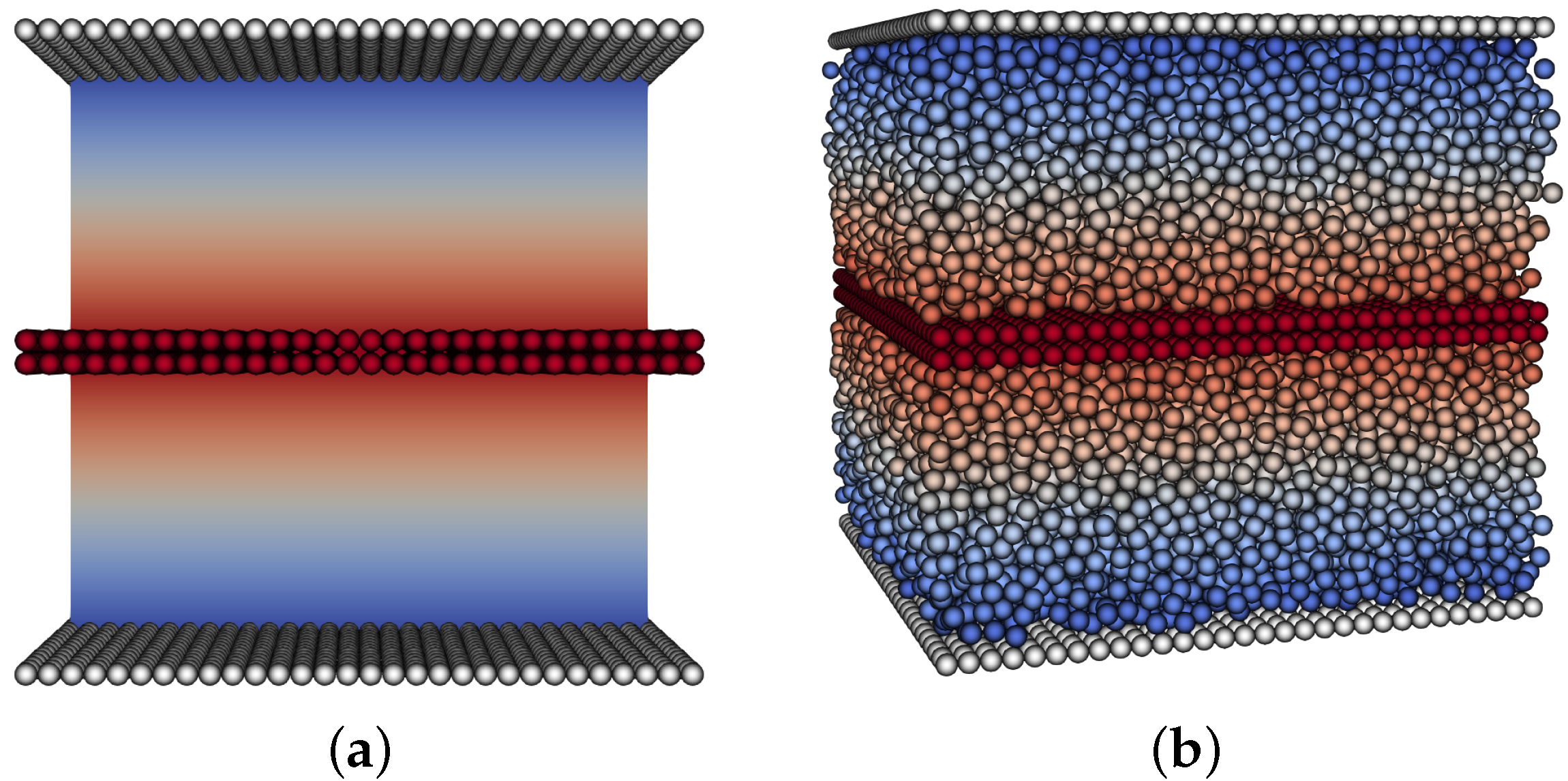
In order to apply the force per unit area on the moving upper plate, we modify the experiment,
Figure 2, and mirror the geometry. Here, both upper and lower boundaries are stationary and there is a layer of particles in the middle that has a force applied in the
x-direction. In order to validate this viscosity measurement, we tested an empty channel and recovered the same viscosity as was set as the fluid parameter.
To measure the viscosity of the simulated particle suspension, we also fix a layer of stationary particles at the bottom and top walls to avoid slip issues at the boundaries.
The shear rates that we want to examine range from 0 to 200 s
, since these levels of rates were measured for red blood cells in biological experiments [
47,
48].
5.2.2. Drag Force Experiment
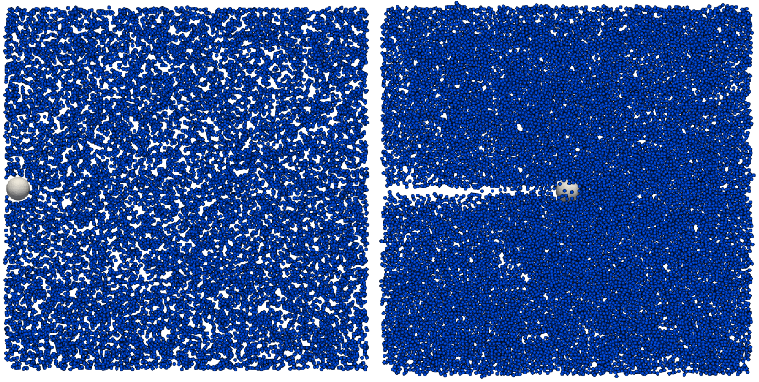
To make a computational analogue to the falling-sphere experiment, we apply force
in the direction of
x-axis to have a sphere moving in a stationary fluid (suspension of soft DPs), see
Figure 3.
The viscosity is then measured, using the Stokes Law, as
where
is the dynamic viscosity,
is the drag force,
R is the radius of the sphere and
v is the (terminal) flow velocity.
This relation holds in an ideal infinite domain. For practical computational purposes, we cannot use periodic boundary conditions since this leads to ever-increasing velocity of the sphere. On the other hand, by imposing solid boundaries, i.e., zero velocity on the boundary, we introduce an artificial boundary effect and the terminal velocity is lower than theoretical. In order to compensate for this, we first evaluate the motion of the sphere in free fluid without particles. In this case, the fluid viscosity is known and thus we can compute the terminal velocity from (
5). Given
nN,
R = 3
m, number of mesh nodes = 304, and
= 1.2 mPas, we calculate the terminal velocity
= 5.894 mms
in infinite domain. We compared different sizes of cube simulation boxes
L to measure the boundary effects,
Table 2.
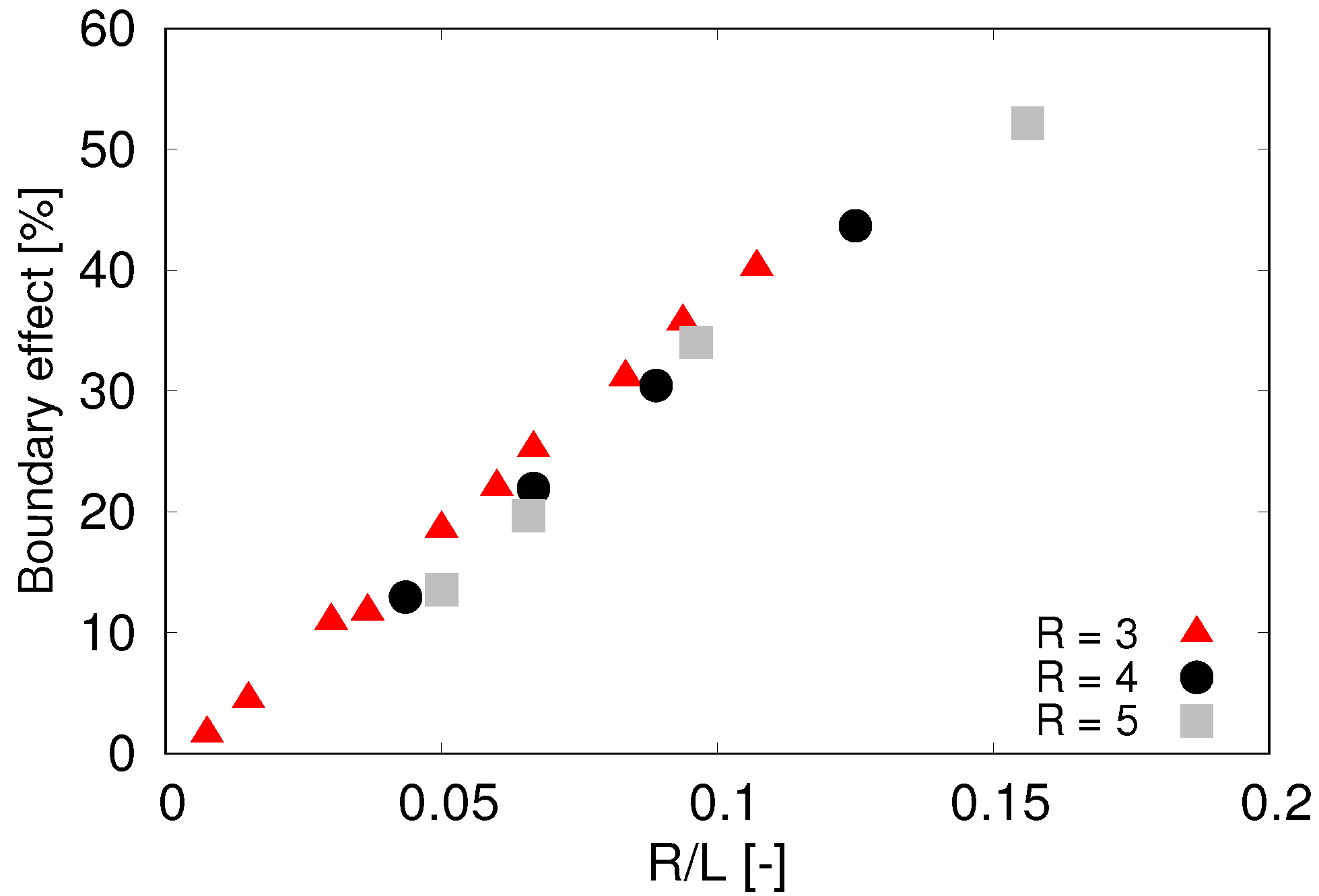
The boundary effect is calculated as relative deviation of computed terminal velocity from the theoretically predicted value
Testing various sizes of the sphere revealed that the effect of the boundary is not fixed to the size
L of the channel but rather to the ratio
of the cell radius and the size of the cross section of the channel. The complete analysis of the boundary effect is presented in
Figure 4 which gives us guidelines how to correct the simulated terminal velocities depending on the ratio of object size and size of the simulation box.
We also tested a range of drag forces 0.05–0.4 nN and two values of fluid viscosity 0.7, 1.2 mPas. These variations had only insignificant impact on the terminal velocity.
Due to the shear thinning properties of particulate suspensions, we need to compare results corresponding to the same shear rates. While in the experiment with two parallel moving plates, the shear rate is explicitly given by the velocity of the moving plates, in the drag force experiment, the shear rate is computed from the fluid velocity gradient near the top and bottom pole of the sphere, assuming horizontal movement of the sphere in the positive x-direction.
The computational complexity of large dense simulations restricts the number of dissipative particles for this computational experiment and implies a lower bound on the radius of the particles. In order to maximize the domain size which reduces the correcting factor depicted in
Figure 4, we performed most computational experiments with particle size
= 0.5
m. For the computational domain 100 × 100 × 100
m
with particle-volume fraction
this accounts for ∼10
particles. A decrease to
= 0.25
m would lead to eight-fold increase in number of particles with the same solid-volume fraction.
5.3. Determining Appropriate Particle-Volume Fraction
Our aim is to reach the viscosity ratio of at least 4. In relation (
4), one can take the values
from [
36] and conclude that we need at least
to have the viscosity contrast close to 4.
Computational experiments for purely conservative forces ( that correspond to no phenomenological viscosity effects in particle suspension) show that it is not possible to have the viscosity ratio higher than two. It is thus clear that we need to also include the dissipative forces. For such forces to have any effect, the pairs of particles need to be closer than the cutoff distance. This fact thus creates a lower bound for . Indeed, if the particle-volume fraction is too low, the particles do not touch and their distance is larger than cutoff distance for dissipative forces and therefore no dissipation is present.
On the other hand, too high value of would make the inter-particle distances smaller than cutoff (effectively meaning an overlap of the DPs) which in turn, in combination with conservative forces, would create a constant tension and make the inner suspension too stiff for a cell to relax back to its original shape.
To determine the appropriate value of particle-volume fraction , we performed the following set of computational experiments for various particle-volume ratios:
Random initialisation of particles inside a 2 × 2 × 2 m domain without boundaries;
Random initialisation of particles inside a 2 × 2 × 2 m domain with boundaries in y and z direction;
Random initialisation of particles inside red blood cell.
The value 2
m was chosen to reflect the thickness of RBC. For all of these we let the suspension relax with conservative forces turned on. We measured the minimal inter-particle distance and number of particle pairs that overlap, i.e., their distance is less than
,
Table 3. Here, we see that the boundaries have a significant effect. The same particle-volume fraction
results in no overlap in the small cubical domain without boundaries, but causes overlap of particles in domain with boundaries. Similarly,
, which is low enough for all particles to relax in cubical domain with or without boundaries is high enough in RBC to cause 513 pairs of particles to overlap. The boundary effect means that there are larger particle-free areas next to boundary than in the middle of the suspension. The RBC with its particularly large surface (boundary) with respect to volume (that helps to transport oxygen in blood) means that the suspension needs to have a lower
. Therefore, in the following, we will consider
and
.
5.4. Considerations for Initial Values of Simulation Parameters
Given the typical ~8
m size of an RBC, we decided to use slightly reduced radius of the sphere
R = 3
m to keep the volume of the sphere closer to that of an RBC. From
Table 2 we see that to keep the correction term from boundary effects close to 10% we need to use ratio
less than
which gives us lower bound for box size
L = 100
m.
From
Table 1 we can see that the viscosity of water and PBS solution ranges from
to 1.2 mPas, while the viscosity of blood plasma ranges from
to 2.2 mPas, depending on the temperature. We will use viscosity of suspending medium
= 1.2 mPas as a mid value.
We will work with the triangulated spheres with 304 nodes and RBCs with 1002 nodes. These triangulations give us the average edge length 0.66 m for sphere with R = 3 m and 0.4 m for the RBC. The fluid in the lattice-Boltzmann method is discretized into a cubical lattice with grid size 1 m.
5.5. Results
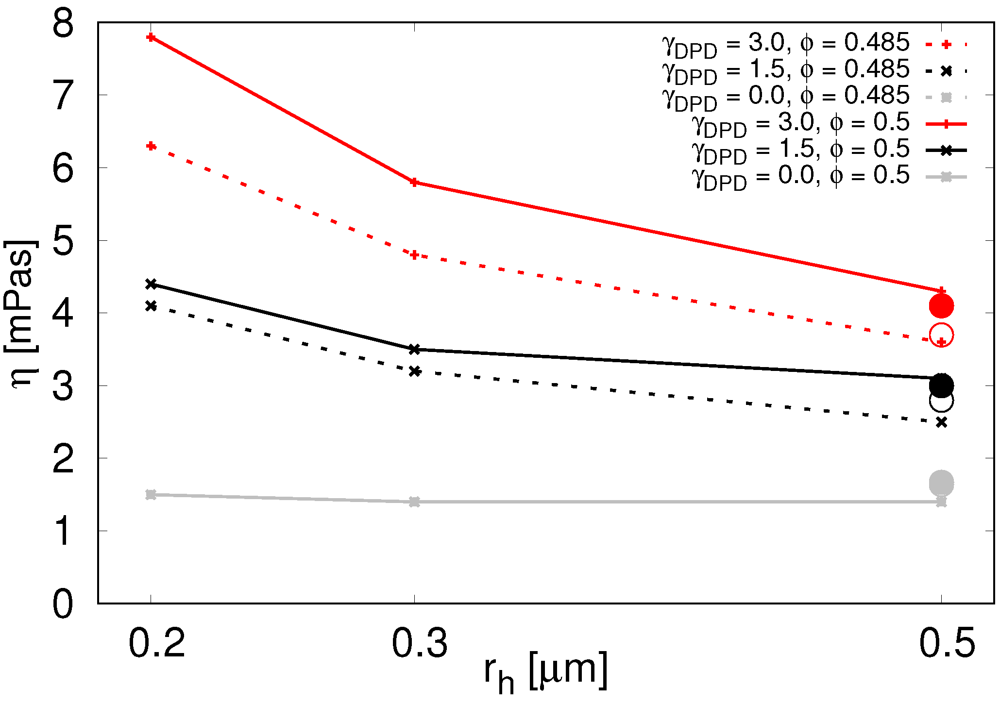
When using the conservative forces alone,
Figure 5 grey line, we see only very slight impact on the effective viscosity at volume fractions around
. The particles rearrange quickly when needed and the desired higher values of viscosity cannot be achieved.
The inclusion of the dissipative forces effectively slows the particles and enables higher viscosity.
With the dissipative forces included, in
Table 4 and
Figure 5 we see that the parallel plate computational experiment and drag force computational experiment give very similar effective viscosity values at
= 0.5
m. Due to significantly larger number of particles needed for simulations with radii small enough to be relevant for inner RBC suspension, we performed only the parallel plate experiment with these, assuming there would be a similar correspondence to the drag force experiment. In the following, we summarize the results from the parallel plate experiment.
In
Figure 5, we see that viscosity increases with decreasing particle radius. This is true for various values of
as well as for various particle volume densities. The second thing we see from
Figure 5 is that viscosity increases with increasing
. This means we can use the parameter
to tune the viscosity contrast.
Next, in
Table 5, we see that for small shear rates there is almost no difference between viscosities measured at different shear rates. The shear-thinning properties of blood manifest at higher shear rates.
Furthermore, finally, there is a steep decline of viscosity for lower particle volume fractions as evidenced in
Table 6. Volume fractions below 45% do not engage the particle dissipative forces enough to raise the viscosity sufficiently.
From these results, we conclude that it is possible to use various combinations of
and
to achieve the desired viscosity ratio. We list some of the suitable combinations in
Table 7.
6. Model Validation
The primary motivation for using inner soft particles was to enable viscosity contrast in red blood cell model. Therefore, we next consider the following computational experiments with red blood cells with inner particle suspension: the gold standard optical tweezers experiment; both the stretching part to observe the elastic response of the membrane and the dynamic release part to observe the viscous response during relaxation.
6.1. Optical Tweezers-Stretching
We performed the computational stretching experiments similar to [
49]. The elastic parameters of the RBC model and other details of the computational experiments were set according to recommendations from [
18]. The final axial and transversal diameters of RBC with dissipative particles stretched with the applied force 0.192 nN (
and
) were 14.2–14.25
m and 4.28–4.54
m, respectively. Data for other stretching forces are available in
Table A6. For all stretching forces the diameters were within the biological data range. This was expected, as this is a static experiment and the particles have larger impact on the dynamics.
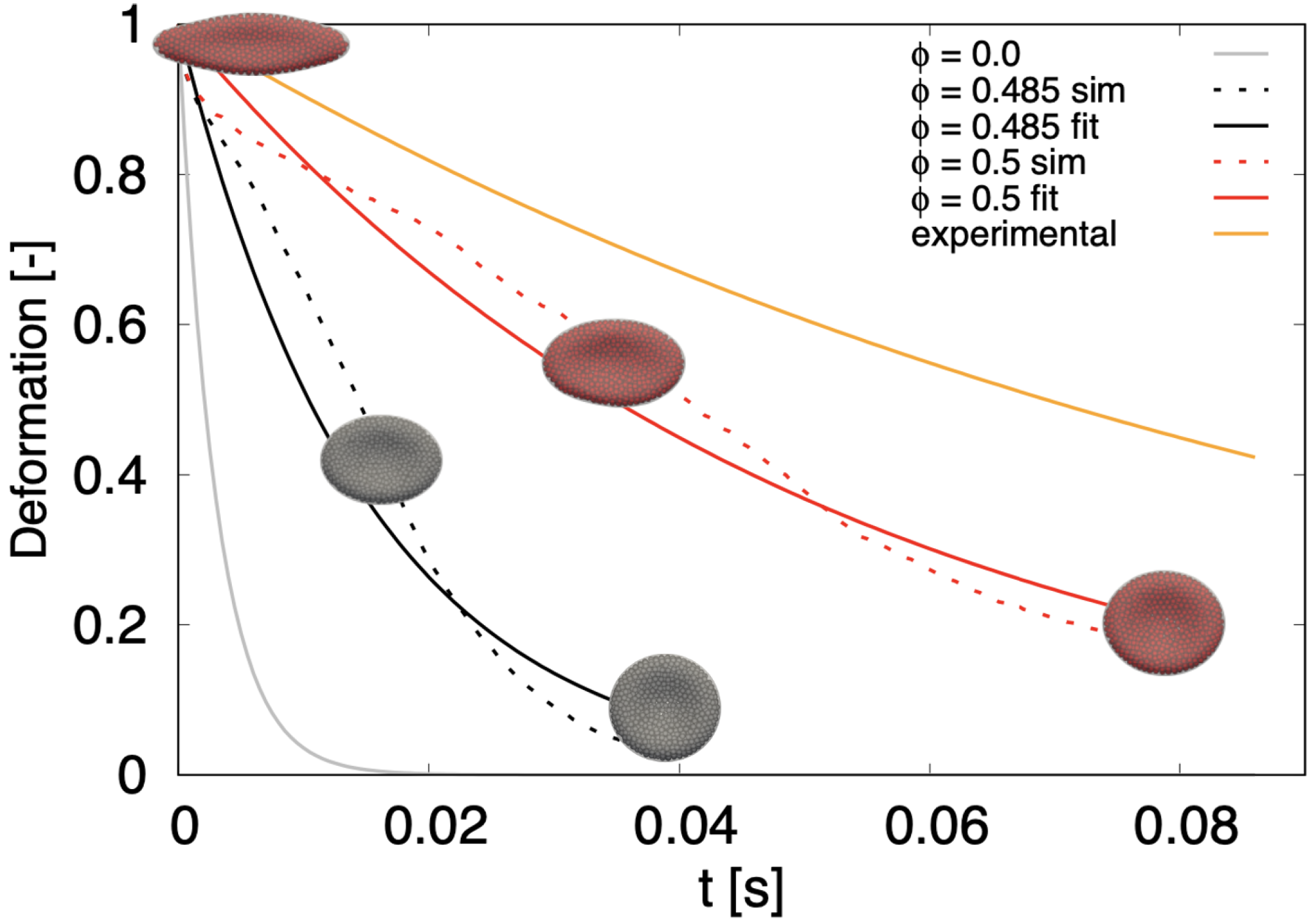
6.2. Optical Tweezers-Release
For the dynamical part of the optical tweezers computational experiment, we released the stretched cells and let them relax back to the original biconcave discoid shape. Similarly to [
49,
50], during the release we calculate the ratio
where
,
is the axial diameter,
is the transversal diameter and
represents the maximum deformation just before the release. In order to compare the return of the cell to the relaxed state, we fitted each time series (
7) with an exponential curve
with characteristic time-constant
. The results are shown in
Figure 6.
The grey line represents the relaxation of a simulated cell without dissipative particles (
) with time constant
s. The orange line represents data from biological experiment [
50]. While the ranges given in the literature vary, the fastest release times shown here correspond to
s. The two dotted lines correspond to computational experiments with particles: black with
and red with
. We see that the larger particle-volume fraction slows the return to relaxed shape more. The respective solid lines represent the exponential fit with
s and
s.
Although the relaxation time of the presented model is lower than time from the biological experiment, we see a significant shift towards the biological data compared to the previous model. Already in [
50] the authors attribute the slow relaxation time to the viscosity of the RBC membrane. We expect that introducing phenomenological viscosity to membrane particles would further prolong the relaxation time towards the values measured in the biological experiment.
7. Discussion
In the present work, we have developed an RBC model that accounts for non-trivial viscosity ratio. We have analyzed the suspensions of dissipative particles that increase the viscosity of the suspending medium in two computational experiments: the parallel plate experiment and drag force experiment. The results of both overlapped and gave us the parameters of soft particle suspension that gives the desired inner cell viscosity. Using these parameters we have filled the membrane model of RBC with DPs and we tested this model. First we performed a static validation test—stretching of an RBC. Then we showed that inclusion of dissipative particles significantly reduced the discrepancy of the membrane RBC model in the computational release experiment. The relaxation time was increased from s for the membrane model to s for RBC model with inner particles, almost reaching biological RBC value of s.
7.1. Model Limitations
Adding DPD particles has improved the performance of the model and achieved a slower relaxation of RBC to its original discoid shape. However, there are still possible improvements and limitations to the extent of its use.
We expect that introducing phenomenological viscosity to the membrane would slow down the relaxation time in the release experiment even further and thus achieve even better agreement with the biological data. The main limitations of our approach lie in the added computational complexity. The use of DPD particles requires using meshes with a larger number of nodes. This increases the computational time and thus this approach is less appropriate for modeling dense RBC suspensions.
The computational complexity is also the reason for performing drag force experiments only with small sized simulation boxes. We have assumed that since we achieved comparable results in the drag force experiment and the shear flow between two plates experiment, the results would be comparable also when using smaller particles in the drag force experiment. We estimated the effect of boundaries in a smaller box using simulations without DPD suspension and this allowed us to remove the effect from the simulation with DPD suspension. However, a more precise validation would have been achieved with the larger simulation box which would require at least an 8-fold increase in computational time. In our opinion the precision gain would not justify the computational time.
7.2. Novelty
The use of LBM for the inner and outer fluid and dissipative particles only for increasing the inner viscosity (as opposed to full DPD) leverages the LBM fixed lattice that is naturally suitable for parallelization and decreases computational time. The increase in inner viscosity is thus an emerging property without the need to solve equations to track the inner points at individual timesteps or detect them anew using ray-casting or similar methods.
The newly developed model proves to be more accurate while maintaining the computational complexity.
Author Contributions
Conceptualization, I.C.; methodology, I.C., I.J. and A.B.; software, I.C., I.J. and A.B.; validation, I.J. and A.B.; formal analysis, I.J. and I.C.; investigation, I.C., I.J. and A.B.; data curation, I.J. and A.B.; writing—original draft preparation, I.C.; writing—review and editing, I.J.; visualization, I.J. and A.B.; supervision, I.C.; project administration, I.C.; funding acquisition, I.C. All authors have read and agreed to the published version of the manuscript.
Funding
This research was supported by Operational Program “Integrated Infrastructure” of the project “Integrated strategy in the development of personalized medicine of selected malignant tumor diseases and its impact on life quality”, ITMS code: 313011V446, co-financed by resources of European Regional Development Fund.
Data Availability Statement
Data are contained within the article.
Conflicts of Interest
The authors declare no conflict of interest.
Abbreviations
The following abbreviations are used in this manuscript:
| RBC | Red blood cell |
| CFL | Cell free layer |
| LBM | Lattice-Boltzmann method |
| IBM | Immersed boundary method |
| IB-DC | Immersed boundary via dissipative coupling |
| DP | Dissipative particles |
| DPD | Dissipative particle dynamics |
Appendix A
Table A1.
Simulation parameters, fluid.
Table A1.
Simulation parameters, fluid.
| LBM Grid [m] | Time Step [s] | Viscosity [mPas] | Density [kg/m] |
|---|
| 1 | 0.05 | 1.2 | 1 |
| | RBC | Sphere |
|---|
| [N/m] | 0.009 | 2 |
| [Nm] | 0.007 | 2 |
| [N/m] | 0.09 | 2 |
| [N/m] | 0.9 | 2 |
| [N/m] | 0.9 | 2 |
| no. of nodes | 1002 | 304 |
| mean edge length [m] | 0.4 | 0.66 |
Table A3.
Simulation parameters, conservative interaction in the particle suspension.
Table A3.
Simulation parameters, conservative interaction in the particle suspension.
| Soft-Sphere | Hat |
|---|
| a | n | |
| 0.00032 | 1.5 | 0.6 |
Table A4.
Simulation parameters, interaction of the particle suspension with the membrane. Outer interaction of suspension in the drag force experiment. Inner interaction of particle suspension with cell membrane from the inside, both drag force
Section 5.2.2 and RBC experiments
Section 6.1 and
Section 6.2.
| Interaction | a* | n* | [m] |
|---|
| inner | 0.02 | 1.5 | |
| outer | 0.128 | 1.5 | |
Table A5.
Effective viscosity of particle suspensions in shear flow between parallel plates. The viscosity of the underlying fluid was 1.2 mPas. For we used the soft-sphere interaction.
Table A5.
Effective viscosity of particle suspensions in shear flow between parallel plates. The viscosity of the underlying fluid was 1.2 mPas. For we used the soft-sphere interaction.
| m] | [nNms] | Shear Rate [s | [mPas] |
|---|
| 0.5 | 0.5 | 0 | 53 | 1.4 |
| 0.5 | 0.3 | 0 | 70 | 1.4 |
| 0.5 | 0.2 | 0 | 83 | 1.5 |
| 0.5 | 0.5 | 1.5 | 86 | 2.8 |
| 0.5 | 0.3 | 1.5 | 71 | 3.5 |
| 0.5 | 0.2 | 1.5 | 57 | 4.4 |
| 0.5 | 0.5 | 3 | 68 | 4.3 |
| 0.5 | 0.3 | 3 | 64 | 5.8 |
| 0.5 | 0.2 | 3 | 65 | 7.8 |
| 0.485 | 0.5 | 0 | 53 | 1.4 |
| 0.485 | 0.3 | 0 | 70 | 1.4 |
| 0.485 | 0.2 | 0 | 85 | 1.5 |
| 0.485 | 0.5 | 1.5 | 77 | 2.5 |
| 0.485 | 0.3 | 1.5 | 84 | 3.2 |
| 0.485 | 0.2 | 1.5 | 98 | 4.1 |
| 0.485 | 0.5 | 3 | 53 | 3.6 |
| 0.485 | 0.3 | 3 | 56 | 4.8 |
| 0.485 | 0.2 | 3 | 56 | 6.3 |
| 0.45 | 0.5 | 3 | 65 | 3.0 |
| 0.45 | 0.3 | 3 | 70 | 3.9 |
| 0.45 | 0.2 | 3 | 64 | 4.7 |
Table A6.
Final axial and transversal diameters in optical tweezers stretching experiment at volume fraction .
Table A6.
Final axial and transversal diameters in optical tweezers stretching experiment at volume fraction .
| [nN] | [m] | [m] |
|---|
| 0 | 7.82 | 7.82 |
| 0.016 | 8.65 | 7.35 |
| 0.031 | 9.38 | 6.90 |
| 0.047 | 10.27 | 6.38 |
| 0.068 | 11.07 | 5.97 |
| 0.088 | 11.70 | 5.59 |
| 0.109 | 12.40 | 5.26 |
| 0.13 | 12.95 | 5.05 |
| 0.15 | 13.24 | 4.87 |
| 0.172 | 13.64 | 4.71 |
| 0.192 | 13.98 | 4.60 |
References
- Evans, E.A.; Skalak, R. Mechanics and Thermodynamics of Biomembranes, 1st ed.; CRC Press: Boca Raton, FL, USA, 1980. [Google Scholar]
- Fischer, T.M. Shape memory of human red blood cells. Biophys. J. 2004, 86, 3304–3313. [Google Scholar] [CrossRef] [Green Version]
- Scotheim, J.; Secomb, T. Red blood cells and other nonspherical capsules in shear flow: Oscillatory dynamics and the tank-treading-to-tumbling transition. Phys. Rev. Lett. 2007, 98, 078301. [Google Scholar] [CrossRef] [Green Version]
- Abkarian, M.; Faivre, M.; Viallat, A. Swinging of red blood cells under shear flow. Phys. Rev. Lett. 2007, 98, 188302. [Google Scholar] [CrossRef] [PubMed] [Green Version]
- Abkarian, M.; Faivre, M.; Viallat, A. Full dynamics of a red blood cell in shear flow. Proc. Natl. Acad. Sci. USA 2012, 109, 20808–20813. [Google Scholar]
- Dasanna, A.K.; Mauer, J.; Gompper, G.; Fedosov, D.A. Importance of viscosity contrast for the motion of erythrocytes in microcapillaries. bioRxiv 2021. [Google Scholar] [CrossRef]
- Lanotte, L.; Mauer, J.; Mendez, S.; Fedosov, D.A.; Fromental, J.M.; Claveria, V.; Nicoud, F.; Gompper, G.; Abkarian, M. Red cells’ dynamic morphologies govern blood shear thinning under microcirculatory flow conditions. Proc. Natl. Acad. Sci. USA 2016, 113, 13289–13294. [Google Scholar] [CrossRef] [PubMed] [Green Version]
- Mauer, J.; Mendez, S.; Lanotte, L.; Nicoud, F.; Abkarian, M.; Gompper, G.; Fedosov, D.A. Flow-Induced Transitions of Red Blood Cell Shapes under Shear. Phys. Rev. Lett. 2018, 121, 118103. [Google Scholar] [CrossRef] [Green Version]
- Yazdani, A.Z.K.; Bagchi, P. Phase diagram and breathing dynamics of a single red blood cell and a biconcave capsule in dilute shear flow. Phys. Rev. E 2011, 84, 026314. [Google Scholar] [CrossRef] [PubMed]
- Cordasco, D.; Yazdani, A.; Bagchi, P. Comparison of erythrocyte dynamics in shear flow under different stress-free configurations. Phys. Fluids 2014, 26, 041902. [Google Scholar] [CrossRef]
- Chien, W.; Gompper, G.; Fedosov, D.A. Effect of cytosol viscosity on the flow behavior of red blood cell suspensions in microvessels. Microcirculation 2021, 28, e12668. [Google Scholar] [CrossRef]
- Mauer, J. Shapes and Dynamics of Blood Cells in Poiseuille and Shear Flows. Ph.D. Thesis, Mathematisch-Naturwissenschaftlichen Fakultat der Universitat zu Kolln, Köln, Germany, 2016. [Google Scholar]
- De Haan, M.; Zavodszky, G.; Azizi, V.; Hoekstra, A.G. Numerical Investigation of the Effects of Red Blood Cell Cytoplasmic Viscosity Contrasts on Single Cell and Bulk Transport Behaviour. Appl. Sci. 2018, 8, 1616. [Google Scholar] [CrossRef] [Green Version]
- Saadat, A.; Guido, C.J.; Shaqfeh, E.S.G. Effect of Cytoplasmic Viscosity on Red Blood Cell Migration in Small Arteriole-level Confinements. bioRxiv 2019. [Google Scholar] [CrossRef]
- Cokelet, G.R.; Meiselman, H.J. Rheological Comparison of Hemoglobin Solutions and Erythrocyte Suspensions. Science 1968, 162, 275–277. [Google Scholar] [CrossRef]
- Wells, R.; Schmid-Schönbein, H. Red cell deformation and fluidity of concentrated cell suspensions. J. Appl. Physiol. 1969, 27, 213–217. [Google Scholar] [CrossRef]
- Jančigová, I.; Kovalčíková, K.; Weeber, R.; Cimrák, I. PyOIF: Computational tool for modelling of multi-cell flows in complex geometries. PLoS Comput. Biol. 2020, 16, 1–21. [Google Scholar] [CrossRef] [PubMed]
- Jančigová, I.; Kovalčíková, K.; Bohiniková, A.; Cimrák, I. Spring-network model of red blood cell: From membrane mechanics to validation. Int. J. Numer. Methods Fluids 2020, 92, 1368–1393. [Google Scholar] [CrossRef]
- Dao, M.; Li, J.; Suresh, S. Molecularly based analysis of deformation of spectrin network and human erythrocyte. Mater. Sci. Eng. C 2006, 26, 1232–1244. [Google Scholar] [CrossRef]
- Wang, T.; Rongin, U.; Xing, Z. A micro-scale simulation of red blood cell passage through symmetric and asymmetric bifurcated vessels. Nat. Sci. Rep. 2016, 6, 20262. [Google Scholar] [CrossRef]
- Ye, T.; Peng, L.; Li, Y. Three-dimensional motion and deformation of a red blood cell in bifurcated microvessels. J. Appl. Phys. 2018, 123, 064701. [Google Scholar] [CrossRef] [Green Version]
- Závodszky, G.; van Rooij, B.; Azizi, V.; Hoekstra, A. Cellular Level In-silico Modeling of Blood Rheology with An Improved Material Model for Red Blood Cells. Front. Physiol. 2017, 8, 563. [Google Scholar] [CrossRef] [Green Version]
- Hsieh, H.J. Numerical simulation of the three-dimensional dynamics of healthy and hardened red blood cells passing through a stenosed microvessel by immersed boundary-lattice Boltzmann method. Eng. Rep. 2020, 3, e12320. [Google Scholar] [CrossRef]
- Krueger, T.; Kusumaatmaja, H.; Kuzmin, A.; Shardt, O.; Silva, G.; Viggen, E.M. The Lattice Boltzmann Method; Springer: Berlin/Heidelberg, Germany, 2016. [Google Scholar]
- Cooling, L. The RBC as a Physiological Object. In Pathobiology of Human Disease; McManus, L.M., Mitchell, R.N., Eds.; Academic Press: San Diego, CA, USA, 2014; pp. 3049–3067. [Google Scholar]
- Richards, F.M. The interpretation of protein structures: Total volume, group volume distributions and packing density. J. Mol. Biol. 1974, 82, 1–14. [Google Scholar] [CrossRef]
- Chatterjee, S.N.; Sadhukhan, P.; Chatterjea, J.B. Electron Microscope Studies on the Haemoglobin Molecules. J. Biophys. Biochem. Cytol. 1961, 10, 113–120. [Google Scholar] [CrossRef] [Green Version]
- Erickson, H. Size and shape of protein molecules at the nanometer level determined by sedimentation, gel filtration, and electron microscopy. Biol. Proced Online 2009, 11, 32–51. [Google Scholar] [CrossRef] [Green Version]
- Groot, R.D.; Warren, P.B. Dissipative particle dynamics: Bridging the gap between atomistic and mesoscopic simulation. J. Chem. Phys. 1997, 107, 4423–4435. [Google Scholar] [CrossRef]
- Lei, H.; Karniadakis, G. Predicting the morphology of sickle red blood cells using coarse-grained models of intracellular aligned hemoglobin polymers. Soft Matter 2012, 8, 4507–4516. [Google Scholar] [CrossRef] [PubMed] [Green Version]
- Li, X.; Li, H.; Chang, H.; Lykotrafitis, G.; Karniadakis, G. Computational biomechanics of human red blood cells in hematological disorders. J. Biomech. Eng. 2017, 139, 0210081–02100813. [Google Scholar] [CrossRef] [PubMed]
- Einstein, A. Berichtigung zu meiner Arbeit: “Eine neue Bestimmung der Molekuldimensionen”. Ann. Der Phys. 1911, 339, 591–592. [Google Scholar] [CrossRef] [Green Version]
- Taylor, G. The viscosity of a fluid containing small drops of another fluid. Proc. R. Soc. Lond. A 1932, 138, 41–48. [Google Scholar]
- Batchelor, G.K. Brownian diffusion of particles with hydrodynamic interaction. J. Fluid Mech. 1976, 74, 1–29. [Google Scholar] [CrossRef] [Green Version]
- Batchelor, G.K. The effect of Brownian motion on the bulk stress in a suspension of spherical particles. J. Fluid Mech. 1977, 83, 97–117. [Google Scholar] [CrossRef]
- Krieger, I.M.; Dougherty, T.J. A Mechanism for Non-Newtonian Flow in Suspensions of Rigid Spheres. Trans. Soc. Rheol. 1959, 3, 137–152. [Google Scholar] [CrossRef]
- Scott, G.D.; Kilgour, D.M. The density of random close packing of spheres. J. Phys. D Appl. Phys. 1969, 2, 863–866. [Google Scholar] [CrossRef]
- Kroupa, M.; Vonka, M.; Soos, M.; Kosek, J. Utilizing the Discrete Element Method for the Modeling of Viscosity in Concentrated Suspensions. Langmuir 2016, 32, 8451–8460. [Google Scholar] [CrossRef] [PubMed] [Green Version]
- Bolintineanu, D.; Grest, G.; Lechman, J.E.A. Particle dynamics modeling methods for colloid suspensions. Comp. Part. Mech. 2014, 1, 321–356. [Google Scholar] [CrossRef] [Green Version]
- Winkler, R.G.; Fedosov, D.A.; Gompper, G. Dynamical and rheological properties of soft colloid suspensions. Curr. Opin. Colloid Interface Sci. 2014, 19, 594–610. [Google Scholar] [CrossRef]
- RheoSense. Viscosity of Plasma and Serum as a Tool for Medical Diagnosis and Research. Technical Report. Available online: rheosense.com (accessed on 2 August 2021).
- Harkness, J. The viscosity of human blood plasma; its measurement in health and disease. Biorheology 1971, 8, 171–193. [Google Scholar] [CrossRef]
- Rand, P.W.; Lacombe, E.; Hunt, H.E.; Austin, W.H. Viscosity of normal human blood under normothermic and hypothermic conditions. J. Appl. Physiol. 1964, 19, 117–122. [Google Scholar] [CrossRef] [PubMed]
- Ditzel, J.; Kampmann, J. Whole-blood viscosity, hematocrit and plasma protein in normal subjects at different ages. Acta Physiol. Scand 1971, 81, 264–268. [Google Scholar] [PubMed]
- Dintenfass, L. Internal Viscosity of the Red Cell and a Blood Viscosity Equation. Nature 1968, 219, 956–958. [Google Scholar] [CrossRef] [PubMed]
- Au, S.H.; Storey, B.D.; Moore, J.C.; Tang, Q.; Chen, Y.L.; Javaid, S.; Sarioglu, A.F.; Sullivan, R.; Madden, M.W.; O’Keefe, R.; et al. Clusters of circulating tumor cells traverse capillary-sized vessels. Proc. Natl. Acad. Sci. USA 2016, 113, 4947–4952. [Google Scholar] [CrossRef] [PubMed] [Green Version]
- Tran-Son-Tay, R.; Sutera, S.P.; Rao, P.R. Determination of red blood cell membrane viscosity from rheoscopic observations of tank-treading motion. Biophys. J. 1984, 46, 65–72. [Google Scholar] [CrossRef] [Green Version]
- Fischer, T.M. Tank-tread frequency of the red cell membrane: Dependence on the viscosity of the suspending medium. Biophys. J. 2007, 93, 2553–2561. [Google Scholar] [CrossRef] [PubMed] [Green Version]
- Mills, J.P.; Qie, L.; Dao, M.; Lim, C.T.; Suresh, S. Nonlinear elastic and viscoelastic deformation of the human red blood cell with optical tweezers. Mol. Cell. Biomech. 2004, 1, 169–180. [Google Scholar]
- Hochmuth, R.M.; Worthy, P.R.; Evans, E.A. Red cell extensional recovery and the determination of membrane viscosity. Biophys. J. 1979, 26, 101–114. [Google Scholar] [CrossRef] [Green Version]
Figure 1.
Visualization of RBC model. (a) triangular mesh modelling the membrane, (b) dissipative particles included inside the membrane.
Figure 1.
Visualization of RBC model. (a) triangular mesh modelling the membrane, (b) dissipative particles included inside the membrane.
Figure 2.
Modified computational shear flow experiment. Both upper and lower boundaries have zero no-slip conditions, with force applied to a layer of particles in the middle. This results in two mirrored sections with linear velocity profiles. (a) no particles, (b) particle volume fraction .
Figure 2.
Modified computational shear flow experiment. Both upper and lower boundaries have zero no-slip conditions, with force applied to a layer of particles in the middle. This results in two mirrored sections with linear velocity profiles. (a) no particles, (b) particle volume fraction .
Figure 3.
Initial position of a sphere in a drag force computational experiment (left). A horizontal force is applied to the sphere, eventually resulting in a steady terminal velocity (right). To visualise the cell movement in the suspension, only a slice (width ±1 m from the central plane of the channel) of the suspensions is rendered. Size of the channel 96 × 96 × 96 m, cell radius R = 3 m.
Figure 4.
Boundary effect—relative deviation of computed terminal velocity from the theoretically predicted value. Sphere radius R given in m.
Figure 4.
Boundary effect—relative deviation of computed terminal velocity from the theoretically predicted value. Sphere radius R given in m.
Figure 5.
Viscosity for various particle radii and
(color coded) at
(solid lines) and
(dotted lines) in parallel plates computational experiment. For
(two gray lines that overlap) we used the soft-sphere interaction between the spherical particles. Data available in
Table A5. The circles represent viscosity values from the drag force computational experiment with
= 0.5
m. Solid circles correspond to
and empty circles to
. Two grey circles almost overlap.
Figure 6.
Relaxation of stretched RBC ( = 0.192 nN) to discoid shape. Dotted lines correspond to simulations with particles, solid lines represent exponential fit, either to experimental data (orange) or to simulation data (gray, black and red). stands for simulation without inner particles.
Figure 6.
Relaxation of stretched RBC ( = 0.192 nN) to discoid shape. Dotted lines correspond to simulations with particles, solid lines represent exponential fit, either to experimental data (orange) or to simulation data (gray, black and red). stands for simulation without inner particles.
Table 1.
Viscosity measurements. Blood is a shear thinning fluid and thus the whole blood viscosity depends on shear rate. The values listed here approximately correspond to the shear rates 70–100 s.
Table 1.
Viscosity measurements. Blood is a shear thinning fluid and thus the whole blood viscosity depends on shear rate. The values listed here approximately correspond to the shear rates 70–100 s.
| | Temperature [C] | Viscosity [mPa.s = cP] |
|---|
| | 20 | 1.00 |
| water | 25 | 0.89 |
| | 37 | 0.69 |
| | 20 | 2.2 [41] |
| blood plasma | 25 | 1.63 [42] |
| | 37 | 1.5 [41] |
| | 20 | ∼10 [43] |
| whole blood | 25 | ∼7 [43] |
| | 37 | ∼5 [44] |
| RBC cytosol | 37 | 3–10 [15,45] |
| PBS | 37 | 0.7 [46] |
Table 2.
Boundary effects—relative deviation of terminal velocity from theoretical value.
Table 2.
Boundary effects—relative deviation of terminal velocity from theoretical value.
| box size L [μm] | 50 | 100 | 200 | 400 |
| 0.06 | 0.03 | 0.015 | 0.0075 |
| [mms | 4.59 | 5.24 | 5.63 | 5.79 |
| boundary effect | % | % | % | % |
Table 3.
Determining the appropriate particle-volume fraction . (m) is the minimal distance of two particles (over 1000 replications), is the maximum (over 1000 replications) number of particle pairs that are closer than , where = 0.2 m.
Table 3.
Determining the appropriate particle-volume fraction . (m) is the minimal distance of two particles (over 1000 replications), is the maximum (over 1000 replications) number of particle pairs that are closer than , where = 0.2 m.
| Cube, No Boundaries | Cube, Boundaries | RBC |
|---|
| | | | | | | | |
| 0.545 | 0.400 | 0 | 0.545 | 0.351 | 93 | 0.503 | 0.371 | 513 |
| 0.503 | 0.400 | 0 | 0.524 | 0.39994 | 3 | 0.485 | 0.389 | 40 |
| 0.461 | 0.400 | 0 | 0.503 | 0.400 | 0 | 0.467 | 0.400 | 0 |
Table 4.
Comparison of effective viscosity [mPas] of particle suspensions in shear flow between parallel plates vs. in drag force experiment. The viscosity of the underlying fluid was 1.2 mPas, = 3 nNms and the radius of DPs was = 0.5 m, shear rate given in .
Table 4.
Comparison of effective viscosity [mPas] of particle suspensions in shear flow between parallel plates vs. in drag force experiment. The viscosity of the underlying fluid was 1.2 mPas, = 3 nNms and the radius of DPs was = 0.5 m, shear rate given in .
| | Parallel Plates | Drag Force Sphere |
|---|
| shear rate | | shear rate | |
| 0.5 | 68 | 4.3 | 39 | 4.1 |
| 0.485 | 53 | 3.6 | 41 | 3.7 |
| 0.45 | 65 | 3.0 | 58 | 2.9 |
Table 5.
At low shear rates, the shear rate has almost no impact on the particle suspension viscosity (here ).
Table 5.
At low shear rates, the shear rate has almost no impact on the particle suspension viscosity (here ).
| | Shear Rate | |
|---|
| [m] | [nNms] | [s] | [mPas] |
|---|
| 0.5 | 3.0 | 27 | 4.4 |
| 0.5 | 3.0 | 68 | 4.3 |
| 0.3 | 3.0 | 36 | 5.7 |
| 0.3 | 3.0 | 64 | 5.8 |
| 0.2 | 1.5 | 57 | 4.4 |
| 0.2 | 1.5 | 113 | 4.4 |
Table 6.
Decrease in effective viscosity of particle suspension with respect to the decreasing volume fraction . Here = 3 nNms, radii given in m.
Table 6.
Decrease in effective viscosity of particle suspension with respect to the decreasing volume fraction . Here = 3 nNms, radii given in m.
| | Viscosity [mPas] |
|---|
| | | |
| 0.5 | 7.8 | 5.8 | 4.3 |
| 0.485 | 6.3 | 4.8 | 3.6 |
| 0.45 | 4.7 | 3.9 | 3.0 |
Table 7.
Parameters of the inner particle suspension for RBC that result in appropriate effective viscosity .
Table 7.
Parameters of the inner particle suspension for RBC that result in appropriate effective viscosity .
| | | |
|---|
| [m] | [nNms] | [mPas] |
|---|
| 0.5 | 0.2 | 2.5 | 6.0 |
| 0.5 | 0.3 | 3.4 | 6.0 |
| 0.485 | 0.2 | 2.75 | 6.0 |
| Publisher’s Note: MDPI stays neutral with regard to jurisdictional claims in published maps and institutional affiliations. |
© 2021 by the authors. Licensee MDPI, Basel, Switzerland. This article is an open access article distributed under the terms and conditions of the Creative Commons Attribution (CC BY) license (https://creativecommons.org/licenses/by/4.0/).


