
Adaptive Notch Filter for Piezo-Actuated Nanopositioning System via Position and Online Estimate Dual-Mode
Abstract
:1. Introduction
- A novel VFF-RLS algorithm based on absolute mean error has been proposed. The VFF varies according to the relative error boundary, which is robust to the noise. It is easy to implement parameters turning and provide good performances of both fast tracking and stability.
- A POEDM method has been developed. The benefit of POEDM is that it combines the open-loop system identification with closed-loop feedback control via a simple structure. By this achievement, it is easy to utilize online estimation of PZT nanopositioning system in real-time to obtain good tracking performance.
2. Modeling and Problem Statement
2.1. Modeling of Piezo-Actuated Nanopositioning System
2.2. Description of the PZT Control Problem
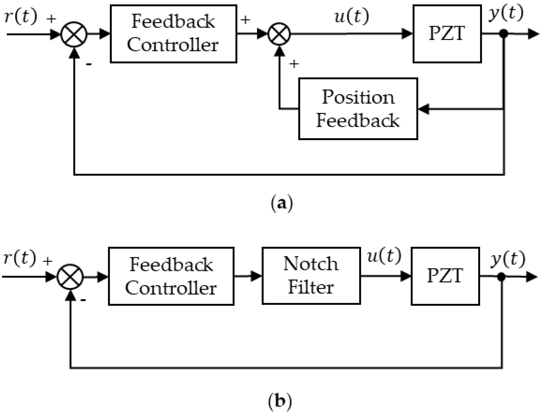
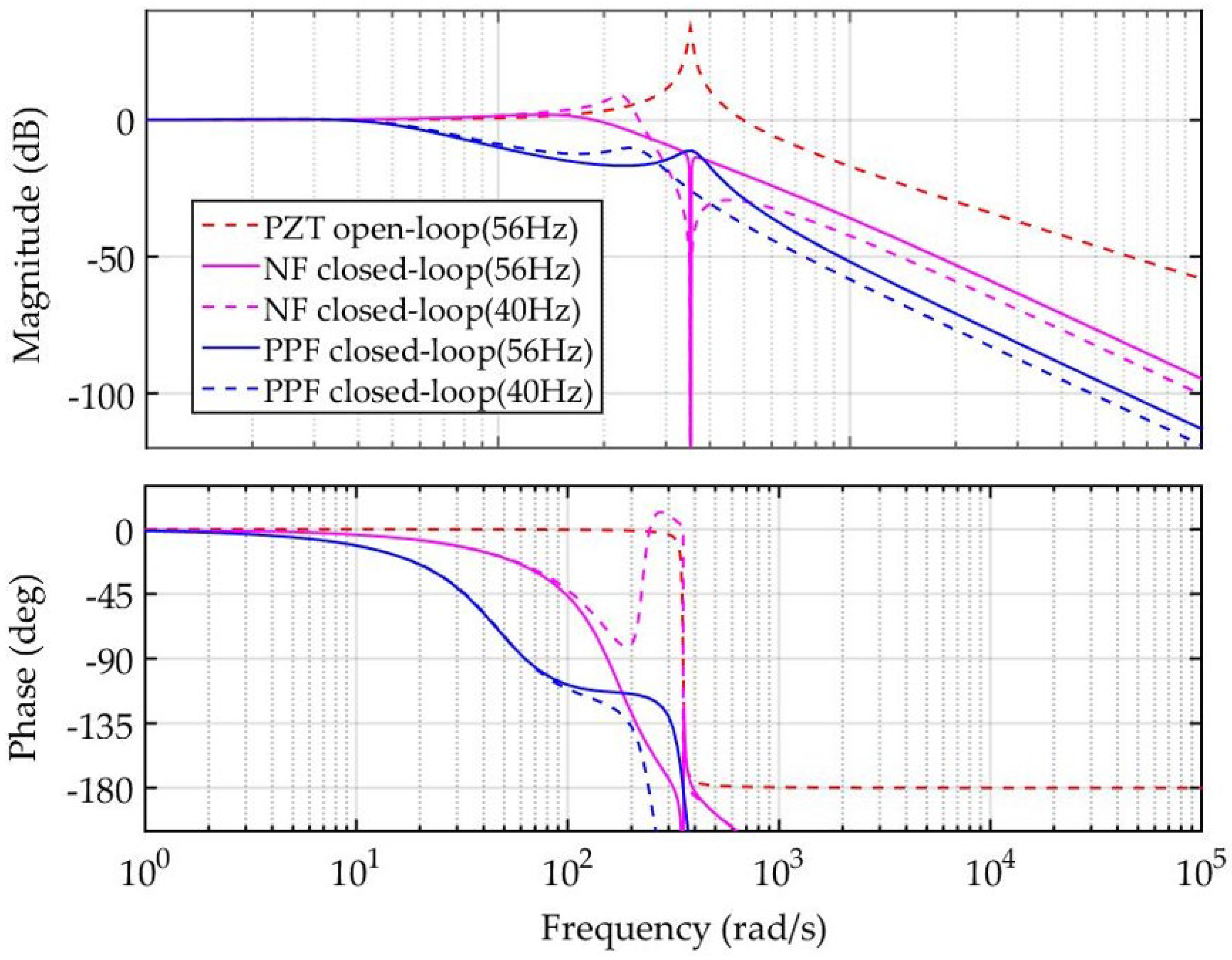
- Position feedback (PF) control, as a type of damping control, increases the damping ratio of system to improve the gain margin via an inner position loop as shown in Figure 1a. Thus, a high gain controller can be used to provide good tracking performance. In addition, since only the position feedback is required, it is easy to be utilized.
- By using NF to eliminate the resonant component in input signal of PZT, the block diagram is shown in Figure 1b. It is designed via inverse model, which is simple to analyze and offers excellent closed-loop bandwidth. By employing NF, the bandwidth is up to or even greater than the resonant frequency [10].
2.3. Description of the Online Frequency Estimate Problem
- a1.
- The order of controller must be high enough;
- a2.
- A nonlinear or time-varying controller is employed;
- a3.
- A large enough delay unit exists in either the forward or feedback path.
- b.
- The disturbance can be formed as a colored noise model.
3. Design of Variable Forgetting Factor RLS Algorithm
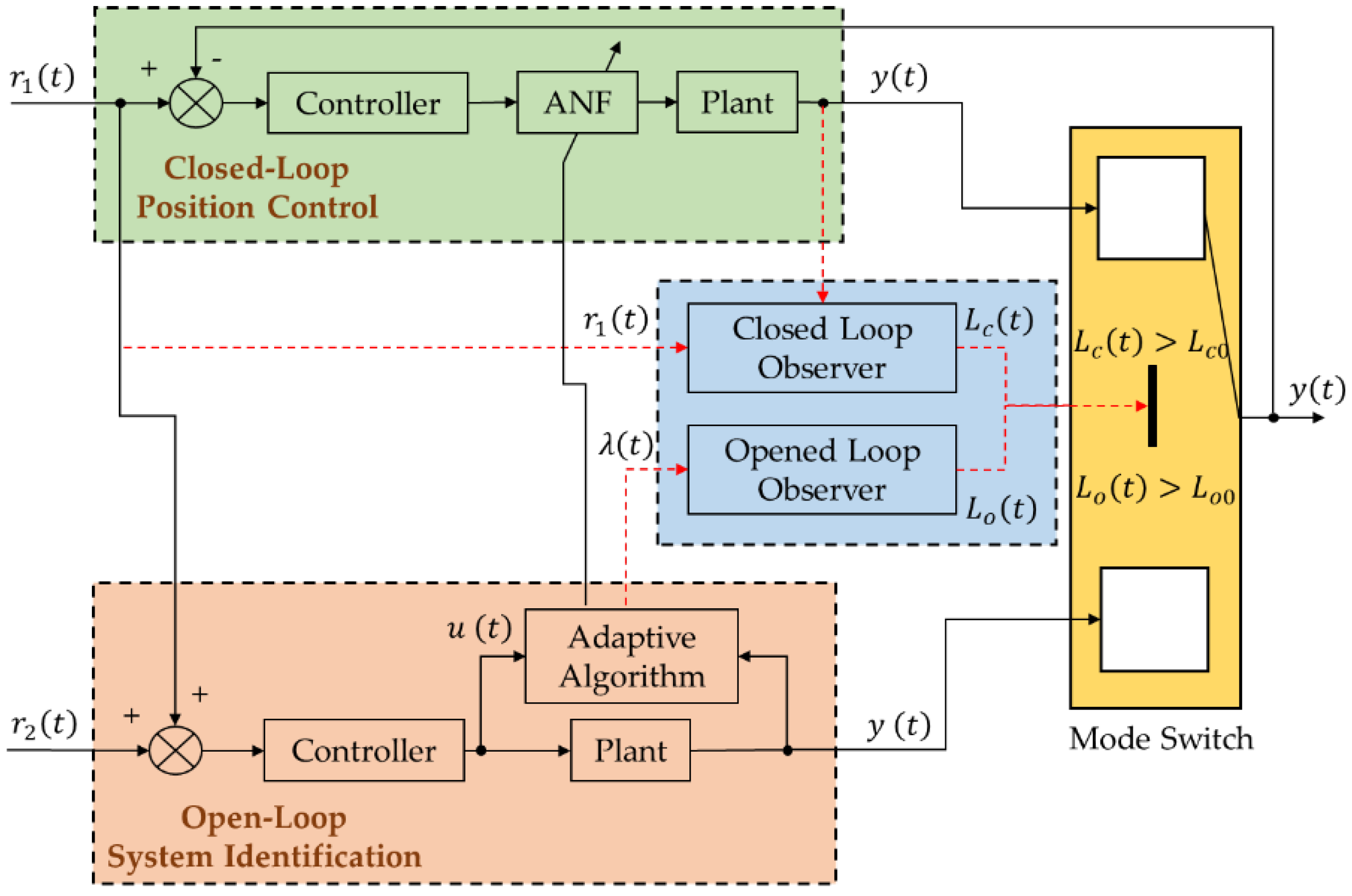
4. Design of Position and Online Estimate Dual-Mode
- The form of closed-loop reference should be set according to the input reference signal. Under the stationary or slowly varying input signal, such as step signal, will not mutate immediately, when the resonant frequency of PZT is varying. In this case, can be defined associate with , in terms of accurate tracking. Then, can be set related to , when input signal is non-stationary or fast varying signal, such as sinusoidal signal. To make it easier to observe the error, the logarithm of can be taken. In summary, can be defined as:where is the error range index and can be set from 1.05 to 1.10. Generally, the stationary signal is adopted in applications, thus the stationary is assumed in this article.
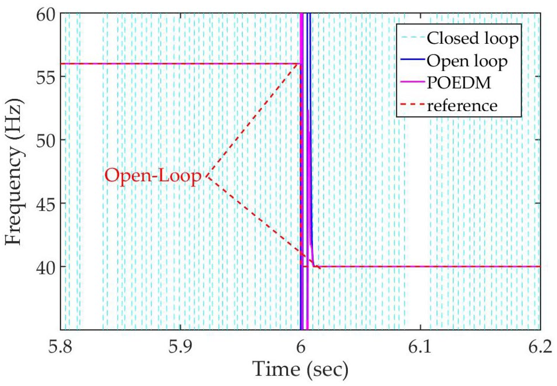
- The form of open-loop reference should be defined associate with . It can be denoted that the identification is completed, when and this will be demonstrated in Section 5.1.
- Identification signal for open-loop system identification is necessary. Due to the disturbance, union error exists in the result of system identification. Aims at reducing the error, an identification signal is required. By using Gaussian noise in , accurate identification result can be obtained. The mean square error of should be defined according to the degree of disturbance. It can be successful to implement identification without , when the frequency components of is enough and the disturbances are not serious.
- Minimum running time of closed-loop and open-loop mode and should be defined, respectively. The state values of mode and may be within their individual reference, caused by the fluctuation. Therefore, a long enough time is needed to ensure that the mode operates fully, where the system will become unstable due to frequent mode switch.
| Algorithm 1 Detailed control Strategy of POEDM. |
| Design Variables: |
| Initialization: |
| Nominal Values: |
5. Simulation Results and Discussion
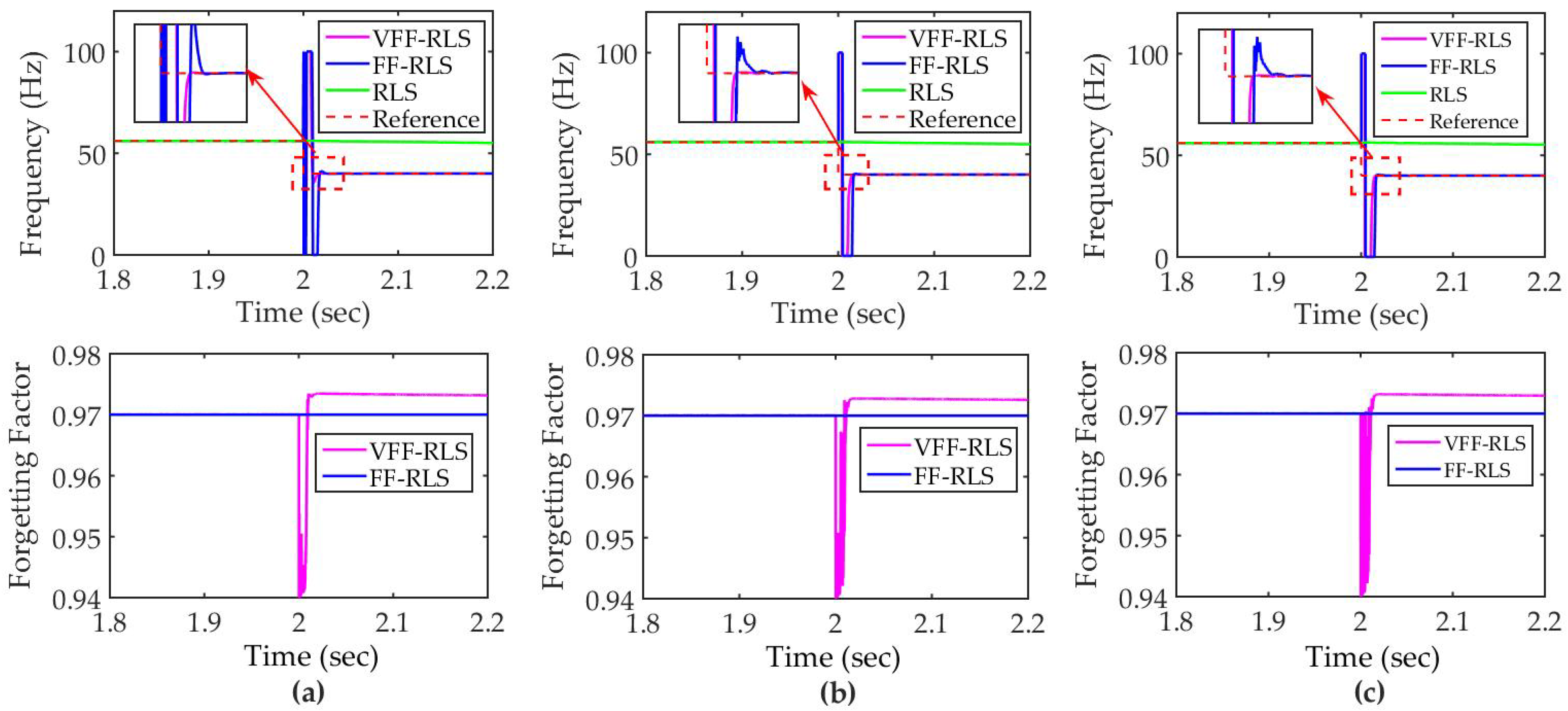
5.1. Variable Forgetting Factor RLS Algorithm Verification
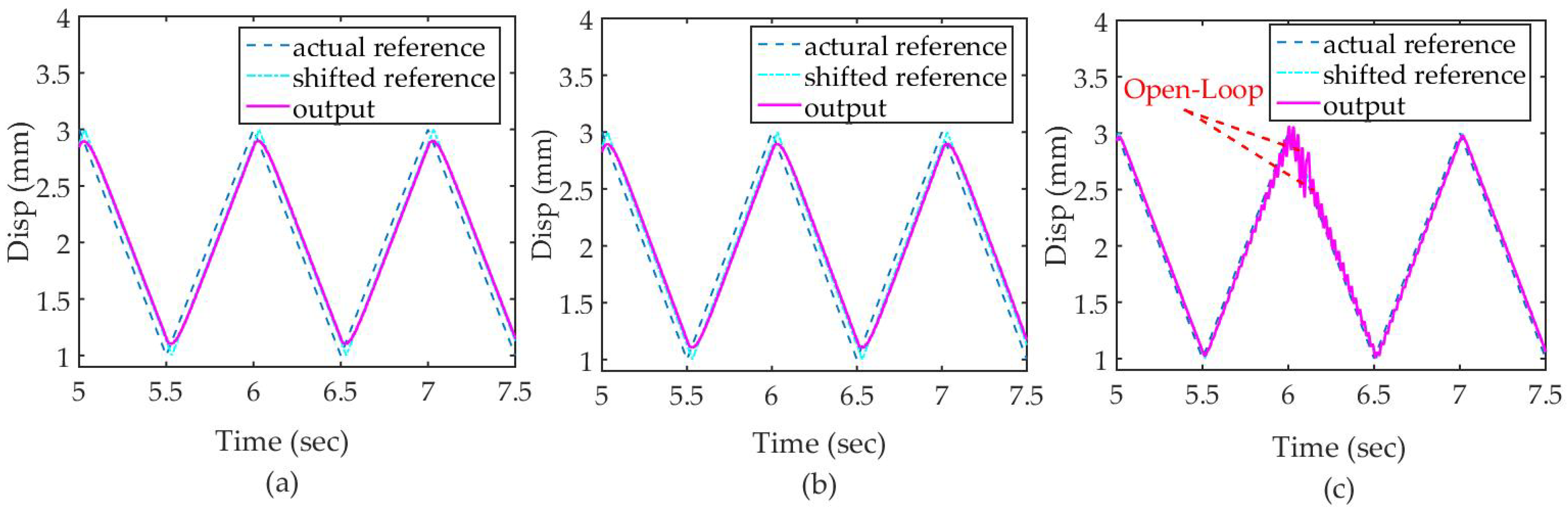
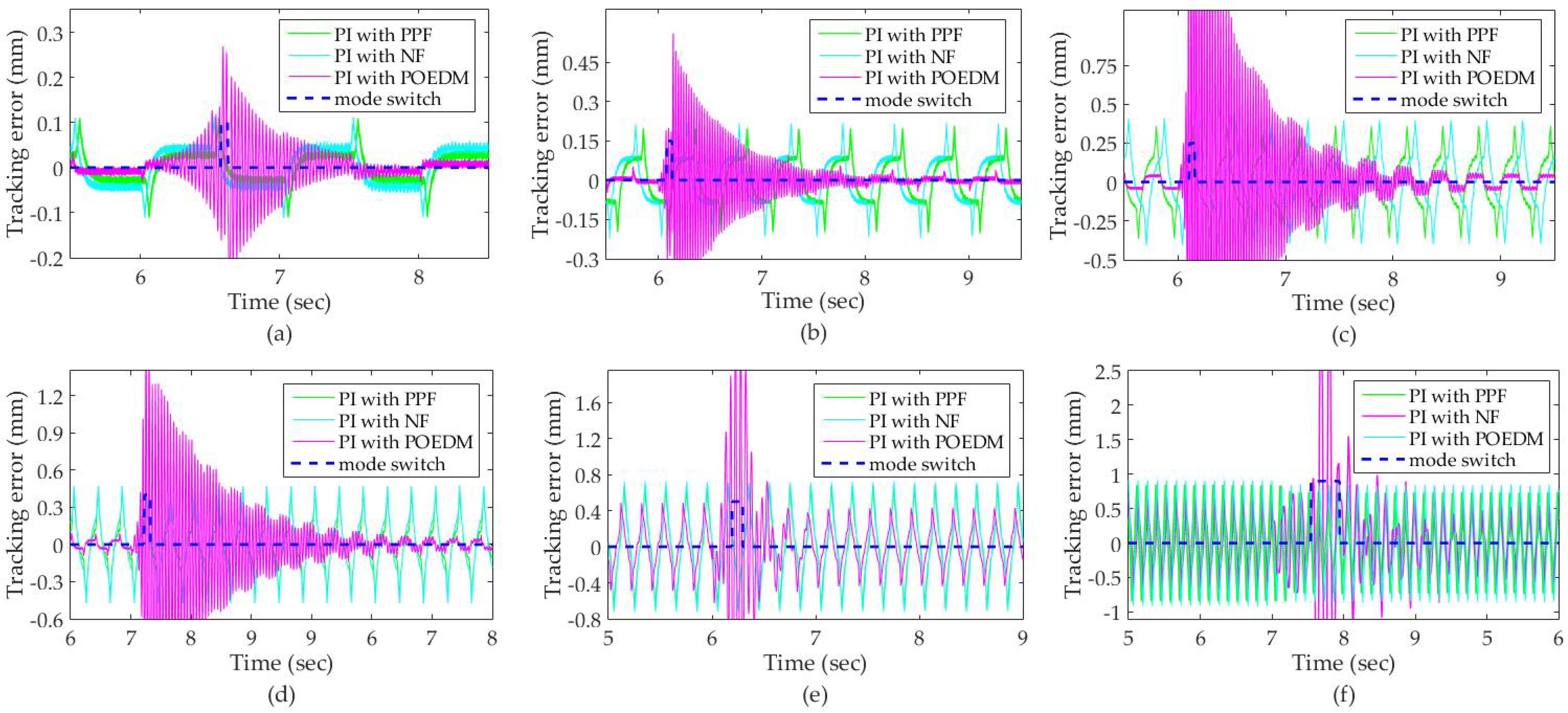
5.2. Position and Online Estimate Dual-Mode Verification
6. Conclusions
Author Contributions
Funding
Data Availability Statement
Conflicts of Interest
References
- Gu, G.; Zhu, L.; Su, C.; Ding, H.; Fatikow, S. Modeling and Control of Piezo-Actuated Nanopositioning Stages: A Survey. IEEE Trans. Autom. Sci. Eng. 2016, 13, 313–332. [Google Scholar] [CrossRef]
- Armin, M.; Roy, P.N.; Das, S.K. A Survey on Modelling and Compensation for Hysteresis in High Speed Nanopositioning of AFMs: Observation and Future Recommendation. Int. J. Autom. Comput. 2020, 17, 479–501. [Google Scholar] [CrossRef]
- Harriott, L.R. Limits of Lithography. Proc. IEEE. 2001, 89, 366–374. [Google Scholar] [CrossRef] [Green Version]
- Fuchs, A.; Vratzov, B.; Wahlbrink, T.; Georgiev, Y.; Kurz, H. Interferometric in situ alignment for UV-based nanoimprint. J. Vac. Sci. Technol. B Microelectron. Nanometer Struct. 2004, 22, 3242–3245. [Google Scholar] [CrossRef]
- Devasia, S.; Eleftheriou, E.; Moheimani, S.O.R. A Survey of Control Issues in Nanopositioning. IEEE Trans. Control Syst. Technol. 2007, 15, 802–823. [Google Scholar] [CrossRef]
- Habibullah, H.; Pota, H.R.; Petersen, I.R. A robust control approach for high-speed nanopositioning applications. Sens. Actuators A Phys. 2019, 292, 137–148. [Google Scholar] [CrossRef]
- Yang, M.; Niu, J.; Li, C.; Gu, G.; Zhu, L. High-Bandwidth Control of Nanopositioning Stages via an Inner-Loop Delayed Position Feedback. IEEE Trans. Autom. Sci. Eng. 2015, 12, 1357–1368. [Google Scholar] [CrossRef]
- Rana, M.S.; Pota, H.R.; Petersen, I.R. High-Speed AFM Image Scanning Using Observer-Based MPC-Notch Control. IEEE Trans. Nanotechnol. 2013, 12, 246–254. [Google Scholar] [CrossRef]
- Eielsen, A.A.; Vagia, M.; Gravdahl, J.T.; Pettersen, K.Y. Damping and Tracking Control Schemes for Nanopositioning. IEEE/ASME Trans. Mechatron. 2014, 19, 432–444. [Google Scholar] [CrossRef] [Green Version]
- Shan, J.; Liu, H.; Sun, D. Slewing and vibration control of a single-link flexible manipulator by positive position feedback (PPF). Mechatronics 2005, 15, 487–503. [Google Scholar] [CrossRef]
- Li, C.; Ding, Y.; Gu, G.; Zhu, L. Damping Control of Piezo-Actuated Nanopositioning Stages With Recursive Delayed Position Feedback. IEEE/ASME Trans. Mechatron. 2017, 22, 855–864. [Google Scholar] [CrossRef]
- Abramovitch, D.; Hoen, S.; Workman, R. Semi-automatic tuning of pid gains for atomic force microscopes. Asian J. Control 2008, 11, 188–195. [Google Scholar] [CrossRef]
- Levin, J.; Perez-Arancibia, N.O.; Ioannou, P.A. Adaptive Notch Filter Using Real-Time Parameter Estimation. IEEE Trans. Control Syst. Technol. 2011, 19, 673–681. [Google Scholar] [CrossRef]
- Ling, J.; Feng, Z.; Ming, M.; Xiao, X. Model reference adaptive damping control for a nanopositioning stage with load uncertainties. Rev. Sci. Instrum. 2019, 90, 045101. [Google Scholar] [CrossRef] [PubMed]
- Nehorai, A. A minimal parameter adaptive notch filter with constrained poles and zeros. IEEE Trans. Acoust. Speech Signal Process. 1985, 33, 1185–1188. [Google Scholar]
- Travassos-Romano, J.; Bellanger, M. Fast least squares adaptive notch filtering. IEEE Trans. Acoust. Speech Signal Process. 1988, 36, 1536–1540. [Google Scholar] [CrossRef]
- Regalia, P. An improved lattice-based adaptive IIR notch filter. IEEE Trans. Signal Process. 1991, 39, 2124–2128. [Google Scholar] [CrossRef]
- Khoshnood, A.; Roshanian, J.; Jafari, A.; Khaki-Sedigh, A. An Adjustable Model Reference Adaptive Control for a Flexible Launch Vehicle. J. Dyn. Syst. Meas. Control 2010, 132, 041010. [Google Scholar] [CrossRef]
- Ohno, K.; Hara, T. Adaptive resonant mode compensation for hard disk drives. IEEE Trans. Ind. Electron. 2006, 53, 624–630. [Google Scholar] [CrossRef]
- Picó, J.; Martínez, M. System Identification. Performance and Closed-Loop Issues; Springer: London, UK, 2002. [Google Scholar]
- Chan, S.; Lin, J.; Sun, X.; Tan, H.; Xu, W. A New Variable Forgetting Factor-Based Bias-Compensation Algorithm for Recursive Identification of Time-Varying Multi-Input Single-Output Systems With Measurement Noise. IEEE Trans. Instrum. Meas. 2020, 69, 4555–4568. [Google Scholar] [CrossRef]
- Deng, J.; Liu, Y.; Zhang, S.; Liu, J. Modeling and experiments of a nano-positioning and high frequency scanning piezoelectric platform based on function module actuator. Sci. China Technol. Sci. 2020, 63, 2541–2552. [Google Scholar] [CrossRef]
- Fleming, A.J.; Leang, K.K. Design, Modeling and Control of Nanopositioning Systems; Springer International Publishing: Cham, Switzerland, 2014. [Google Scholar]
- Leang, K.K.; Zou, Q.; Devasia, S. Feedforward control of piezoactuators in atomic force microscope systems. IEEE Control Syst. 2009, 29, 70–82. [Google Scholar] [CrossRef]
- Omidbeike, M.; Teo, Y.R.; Yong, Y.K.; Fleming, A.J. Tracking control of a monolithic piezoelectric nanopositioning stage using an integrated sensor. IFAC-PapersOnLine 2017, 50, 10913–10917. [Google Scholar] [CrossRef]
- Wen, Z.; Ding, Y.; Liu, P.; Ding, H. An Efficient Identification Method for Dynamic Systems With Coupled Hysteresis and Linear Dynamics: Application to Piezoelectric-Actuated Nanopositioning Stages. IEEE/ASME Trans. Mechatron. 2019, 24, 326–337. [Google Scholar] [CrossRef]
- Ljung, L. System Identification: Theory for the User; Prentice Hall: Hoboken, NJ, USA, 2002. [Google Scholar]
- Fleming, A.J.; Leang, K.K. Charge drives for scanning probe microscope positioning stages. Ultramicroscopy 2008, 108, 1551–1557. [Google Scholar] [CrossRef] [PubMed]
- Butterworth, J.A.; Pao, L.Y.; Abramovitch, D.Y. A Discrete-Time Single-Parameter Combined Feedforward/Feedback Adaptive-Delay Algorithm With Applications to Piezo-Based Raster Tracking. IEEE Trans. Control Syst. Technol. 2012, 20, 416–423. [Google Scholar] [CrossRef]


| Signal | SNR (dB) | RLS | FF-RLS | VFF-RLS | |||
|---|---|---|---|---|---|---|---|
| ST (sec) | MSE | ST (sec) | MSE | ST (sec) | MSE | ||
| Sinusoid | 40 | N/A | 7.397 | 2.048 | 0.43 | 2.028 | 0.368 |
| 50 | N/A | 7.28 | 2.042 | 0.285 | 2.021 | 0.226 | |
| 60 | N/A | 7.244 | 2.031 | 0.24 | 2.018 | 0.181 | |
| Step | 40 | N/A | 7.236 | 2.034 | 0.465 | 2.015 | 0.42 |
| 50 | N/A | 7.156 | 2.032 | 0.27 | 2.014 | 0.237 | |
| 60 | N/A | 7.13 | 2.031 | 0.221 | 2.014 | 0.189 | |
| Ramp | 40 | N/A | 7.28 | 2.045 | 0.385 | 2.017 | 0.355 |
| 50 | N/A | 7.205 | 2.035 | 0.26 | 2.016 | 0.231 | |
| 60 | N/A | 7.182 | 2.028 | 0.221 | 2.016 | 0.192 | |
| Signal (Hz) | PI with PPF | PI with NF | PI with POEDM | ||||
|---|---|---|---|---|---|---|---|
| em (%) | erms (%) | em (%) | erms (%) | em (%) | em-cl (%) | erms (%) | |
| 1 | 5.5 | 1.5 | 5.8 | 2.1 | 13.3 | 1.5 | 1.1 |
| 2 | 10.1 | 3.1 | 10.8 | 4.6 | 28.2 | 1.9 | 2.5 |
| 5 | 22.2 | 7.6 | 24.1 | 9.3 | 85.2 | 3.6 | 4.6 |
| 10 | 34.0 | 14.2 | 35.5 | 15.7 | 143.5 | 23.5 | 11.2 |
| 30 | 41.5 | 19.2 | 45.8 | 20.5 | 225.0 | 36.0 | 18.2 |
| Signal (Hz) | PI with POEDMC | |||
|---|---|---|---|---|
| tc0 (sec) | Actual tc (sec) | to0 (sec) | Actual to (sec) | |
| 1 | 2 | 6.68 | 0.05 | 0.05 |
| 2 | 2 | 6.08 | 0.05 | 0.05 |
| 3 | 2 | 6.1 | 0.05 | 0.05 |
| 5 | 2 | 6.11 | 0.05 | 0.05 |
| 10 | 3 | 6.09 | 0.05 | 0.05 |
| 30 | 3 | 6.14 | 0.1 | 0.76 |
Publisher’s Note: MDPI stays neutral with regard to jurisdictional claims in published maps and institutional affiliations. |
© 2021 by the authors. Licensee MDPI, Basel, Switzerland. This article is an open access article distributed under the terms and conditions of the Creative Commons Attribution (CC BY) license (https://creativecommons.org/licenses/by/4.0/).
Share and Cite
Huang, C.; Li, H. Adaptive Notch Filter for Piezo-Actuated Nanopositioning System via Position and Online Estimate Dual-Mode. Micromachines 2021, 12, 1525. https://doi.org/10.3390/mi12121525
Huang C, Li H. Adaptive Notch Filter for Piezo-Actuated Nanopositioning System via Position and Online Estimate Dual-Mode. Micromachines. 2021; 12(12):1525. https://doi.org/10.3390/mi12121525
Chicago/Turabian StyleHuang, Chengsi, and Hongcheng Li. 2021. "Adaptive Notch Filter for Piezo-Actuated Nanopositioning System via Position and Online Estimate Dual-Mode" Micromachines 12, no. 12: 1525. https://doi.org/10.3390/mi12121525
APA StyleHuang, C., & Li, H. (2021). Adaptive Notch Filter for Piezo-Actuated Nanopositioning System via Position and Online Estimate Dual-Mode. Micromachines, 12(12), 1525. https://doi.org/10.3390/mi12121525