
Space Detumbling Robot Arm Deployment Path Planning Based on Bi-FMT* Algorithm


Abstract
:1. Introduction
2. Space Detumbling Robot Modeling
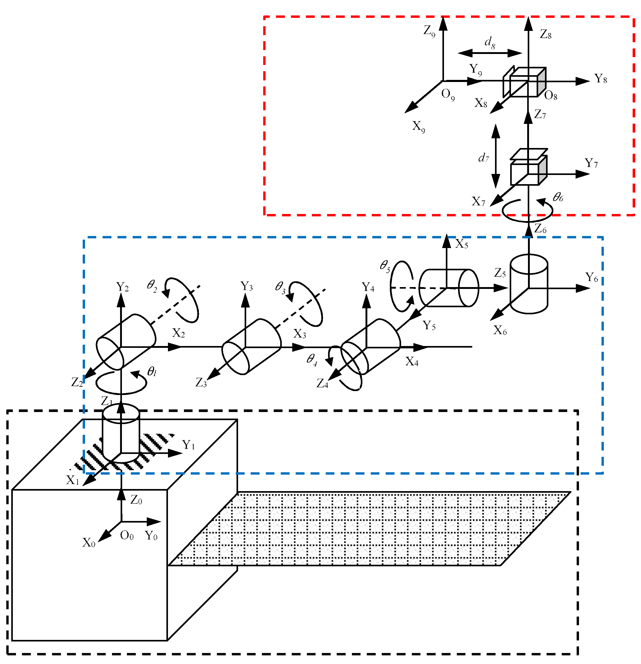
2.1. Kinematics
- (1)
- Oi+1Xi+1 is perpendicular to OiZi;
- (2)
- Oi+1Xi+1 intersects with OiZi.
2.2. Dynamics
3. Space Detumbling Robot Arm Path Planning Based on Bi-FMT* Algorithm
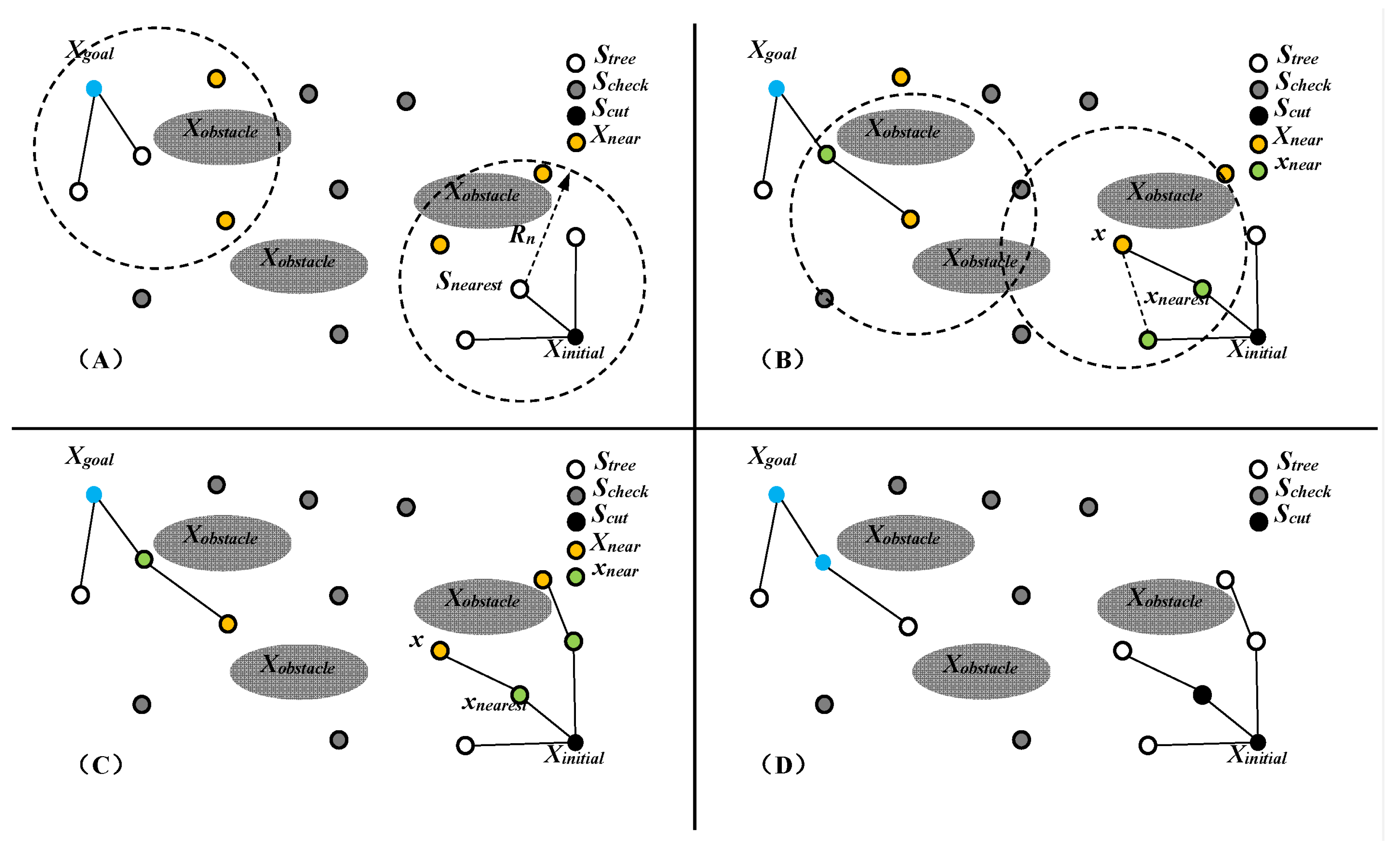
3.1. Bi-FMT* Algorithm
3.2. Problem Definition
| Given: | Θinitial, t0, Θgoal, Θfree |
| Cost function: | |
| Constraints: |
3.3. Constraint Analysis
3.3.1. Time Constraints
3.3.2. Stationary Constraints
3.3.3. Dynamic Characteristic Constraints
3.4. Path Planning Algorithm Description
4. Simulation
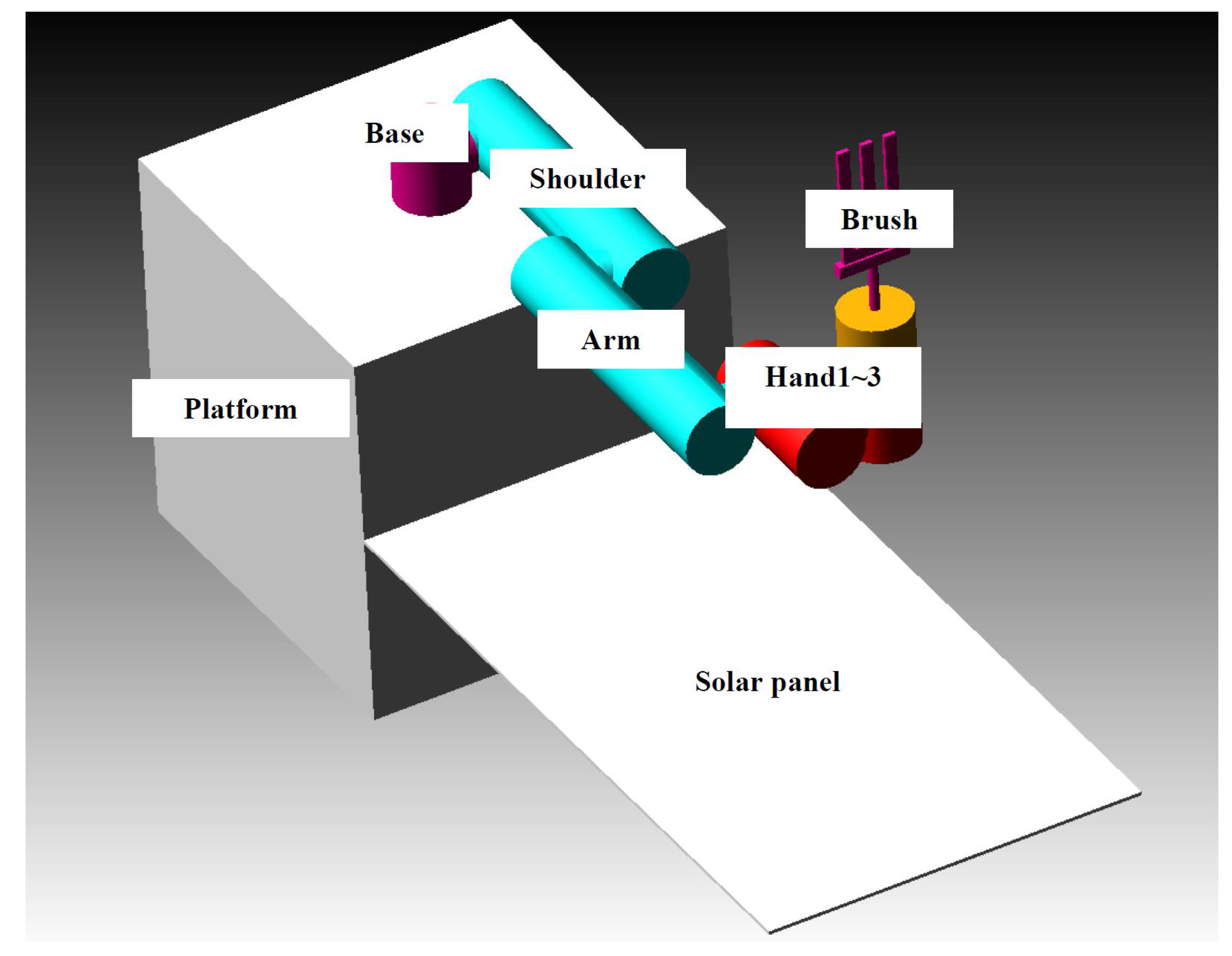
4.1. Robot Model
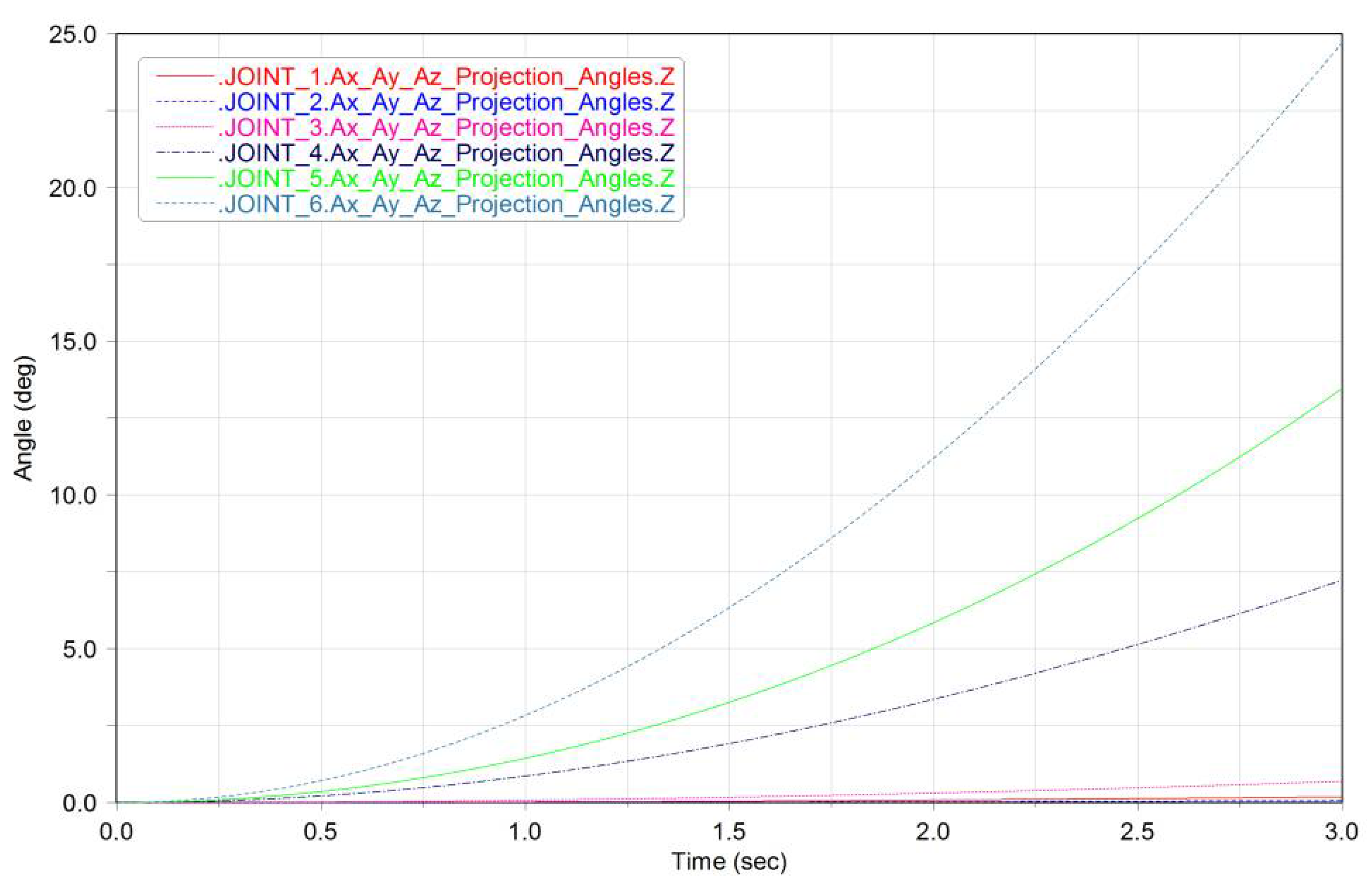
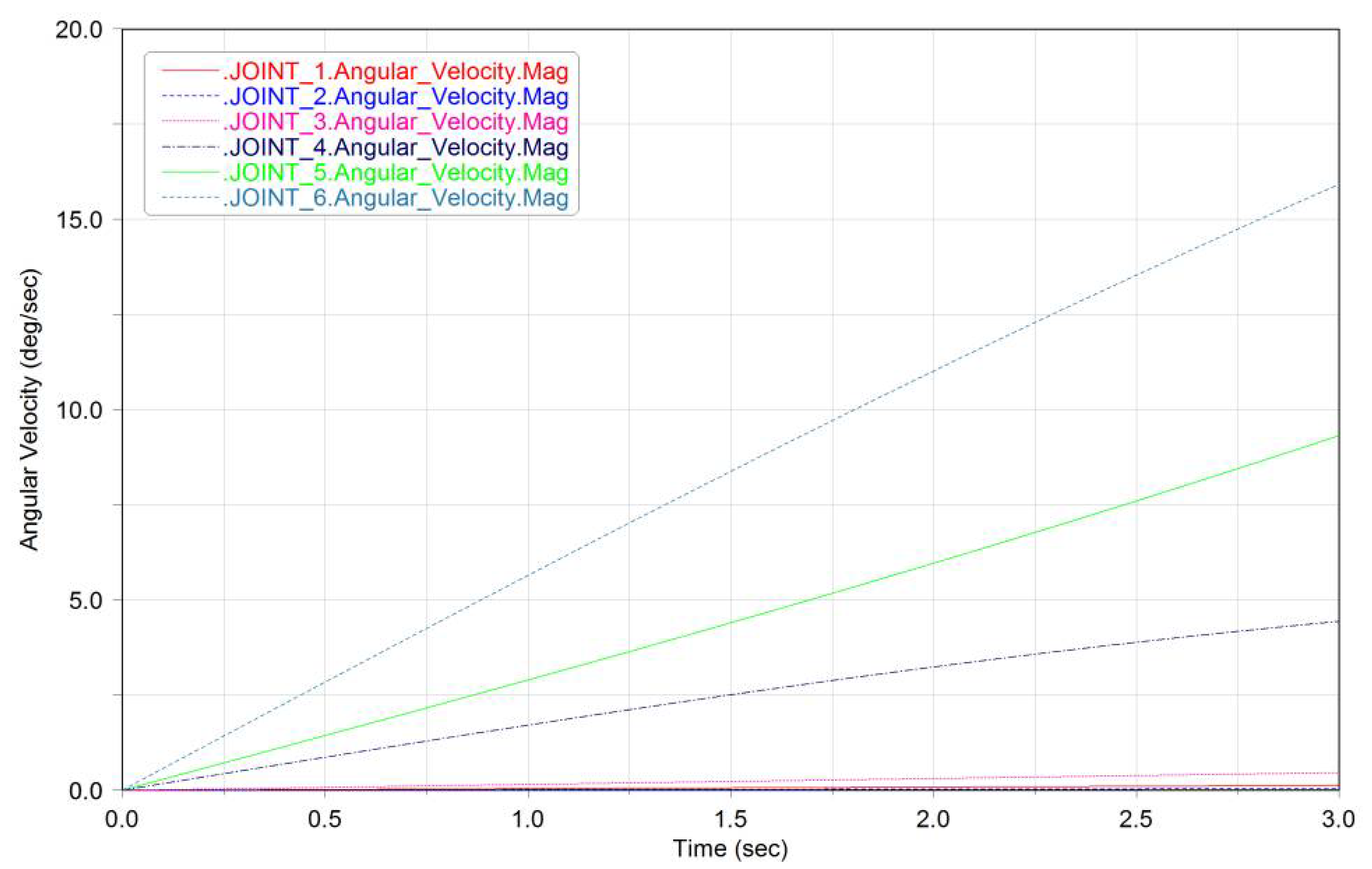
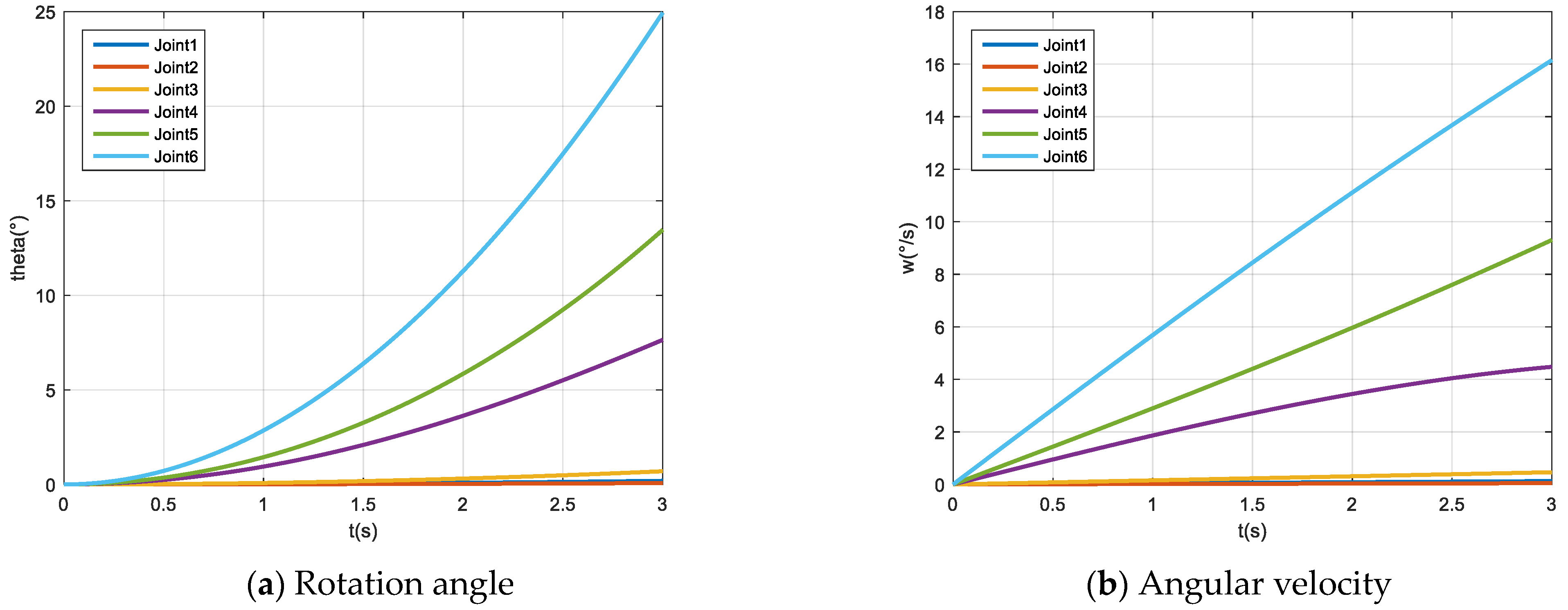
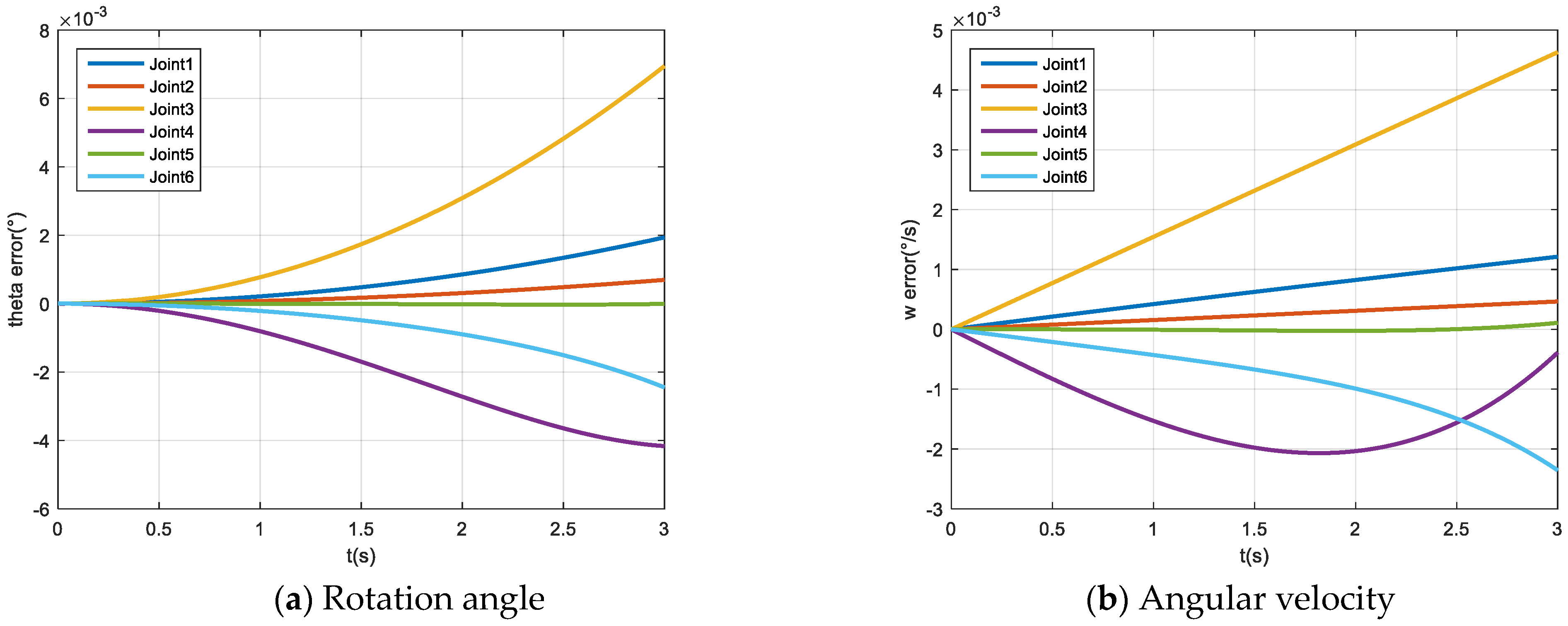
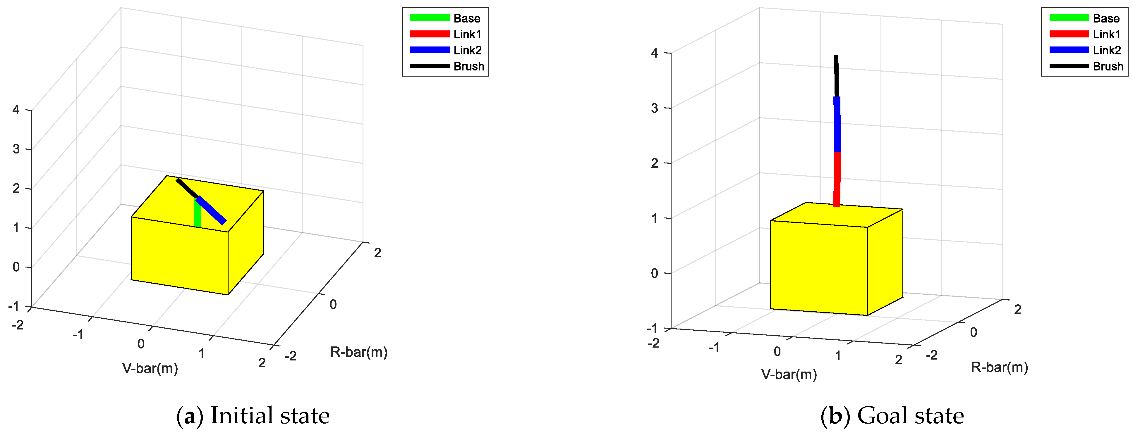
4.2. Path Planning
5. Conclusions and Future Work
Author Contributions
Funding
Data Availability Statement
Conflicts of Interest
References
- Yingzi, H.; Chunling, W.; Liang, T. Research status and development trend of space control technology. Space Control. Technol. Appl. 2014, 40, 1–8. [Google Scholar]
- Ning, C.; Yasheng, Z.; Wenhua, C. Review and Outlook of the Space Operation and Control Project Development and Technology. In Proceedings of the 3rd International Conference on Unmanned Systems (ICUS), Harbin, China, 27–28 November 2020. [Google Scholar]
- Weilin, W.; Yangang, L. Guidance and control for satellite proximity operations. Aircr. Eng. Aerosp. Technol. 2014, 86, 76–86. [Google Scholar]
- Bonnal, C.; Ruault, J.M.; Desjean, M.C. Active debris removal: Current status of activities in CNES. In Proceedings of the 6th European Conference on Space Debris, Darmstadt, Germany, 22–25 April 2013. [Google Scholar]
- Nao, T.; Hirohisa, K. Autonomous learning-type impact thrust method for damping angular momentum of malfunctioning satellites. Proc. Jpn. Aerosp. Soc. 2007, 55, 27–33. [Google Scholar]
- Ferrari, F.; Benvenuto, R.; Lavagna, M. Gas plume impingement technique for space debris de-tumbling. In Proceedings of the International ESA Conference on Guidance, Navigation & Control Systems, Oporto, Portugal, 2–6 June 2014. [Google Scholar]
- Kumar, R.; Sedwick, R.J. Despinning Orbital Debris Before Docking Using Laser Ablation. J. Spacecr. Rocket. 2015, 52, 1129–1134. [Google Scholar] [CrossRef]
- Vetrisano, M.; Thiry, N.; Vasile, M. Detumbling large space debris via laser ablation. In Proceedings of the IEEE Aerospace Conference, Big Sky, MT, USA, 7–14 March 2015. [Google Scholar]
- Caubet, A.; Biggs, J.D. Design of an attitude stabilization electromagnetic module for detumbling uncooperative targets. In Proceedings of the IEEE Aerospace Conference, Big Sky, MT, USA, 1–8 March 2014. [Google Scholar]
- Yudintsev, V.; Aslanov, V. Detumbling Space Debris Using Modified Yo-Yo Mechanism. J. Guid. Control. Dyn. 2017, 40, 1–8. [Google Scholar] [CrossRef]
- Zhang, S.; Luo, Z.; Nie, T.; Gu, Y.; Jiang, Y.; Fan, Y. Fast Rolling Target Derotating Cell Sail for On-Orbit Service and Its Working Method. Invention Patent CN105197261A, 2015. [Google Scholar]
- Bennett, T.; Schaub, H. Capitalizing on relative motion in electrostatic de-tumbling of axisymmetric GEO objects. In Proceedings of the 6th International Conference on Astrodynamics Tools and Techniques (ICATT), Darmstadt, Germany, 14–17 March 2016. [Google Scholar]
- Bennett, T.; Stevenson, D.; Hogan, E.; Schaub, H. Prospects and challenges of touchless electrostatic detumbling of small bodies. Adv. Space Res. 2015, 56, 557–568. [Google Scholar] [CrossRef]
- Zhao, Y. Research on Non-Contact Attitude Control Based on the Coulomb Force. Ph.D. Thesis, Harbin Institute of Technology, Harbin, China, 2016. [Google Scholar]
- Bennett, T.; Schaub, H. Touchless electrostatic de-tumble of a representative box-and-panel spacecraft configuration. In Proceedings of the 7th European Conference on Space Debris, Darmstadt, Germany, 18–21 April 2017. [Google Scholar]
- Kadaba, P.K.; Naishadham, K. Feasibility of noncontacting electromagnetic de-spinning of a satellite by inducing eddy currents in its skin. I. Analytical considerations. IEEE Trans. Magn. 2002, 31, 2471–2477. [Google Scholar] [CrossRef]
- Sugai, F.; Abiko, S.; Tsujita, T.; Jiang, X.; Uchiyama, M. De-tumbling an uncontrolled satellite with contactless force by using an eddy current brake. In Proceedings of the International Conference on Intelligent Robots and Systems, Hamburg, Germany, 28 September–2 October 2015. [Google Scholar]
- Gómez, N.O.; Walker, S.J.I. Eddy currents applied to de-tumbling of space debris: Analysis and validation of approximate proposed methods. Acta Astronaut. 2015, 114, 34–53. [Google Scholar] [CrossRef] [Green Version]
- Jankovic, M.; Kumar, K.; Gómez, N.O. Spacecraft concept for active de-tumbling and robotic capture of Ariane rocket bodies. In Proceedings of the 13th Symposium on Advanced Space Technologies in Robotics and Automation, Noordwijk, The Netherlands, 10–13 May 2015. [Google Scholar]
- Figura, J.S.; James, N. A laboratory demonstration of de-tumbling space debris with magnetically-induced eddy current torques. In Proceedings of the 1st IAA Conference on Space Situational Awareness, Orlando, FL, USA, 13–15 November 2017. [Google Scholar]
- Nishida, S.I.; Kawamoto, S. Strategy for capturing of a tumbling space debris. Acta Astronaut. 2011, 68, 113–120. [Google Scholar] [CrossRef]
- Matunaga, S.; Kanzawa, T.; Ohkami, Y. Rotational motion-damper for the capture of an uncontrolled floating satellite. Control. Eng. Pract. 2001, 9, 199–205. [Google Scholar] [CrossRef]
- Kawamoto, S.; Matsumoto, K.; Wakabayashi, S. Ground experiment of mechanical impulse method for uncontrollable satellite capturing. In Proceedings of the 6th International Symposium on Artificial Intelligence and Robotics & Automation in Space (i-SAIRAS), St-Hubert, QC, Canada, 18–22 June 2001; pp. 1–8. [Google Scholar]
- Huang, P.; Zhang, F.; Meng, Z.; Liu, Z. Adaptive control for space debris removal with uncertain kinematics, dynamics and states. Acta Astronaut. 2016, 128, 416–430. [Google Scholar] [CrossRef]
- O’Connor, W.J.; Hayden, D.J. De-tumbling of space debris by a net and elastic tether. J. Guid. Control. Dyn. 2017, 40, 1829–1836. [Google Scholar] [CrossRef]
- Shan, M.; Guo, J.; Gill, E. Tumbling space debris capturing using a net. In Proceedings of the 7th European Conference on Space Debris, Darmstadt, Germany, 18–21 April 2017. [Google Scholar]
- Hovell, K.; Ulrich, S. Attitude stabilization of an uncooperative spacecraft in an orbital environment using visco-elastic tethers. In Proceedings of the AIAA Guidance, Navigation, and Control Conference, Kissimmee, FL, USA, 5–9 January 2015. [Google Scholar]
- Velez, P.; Atie, T.; Alazard, D.; Cumer, C. Space Debris Removal using a Tether: A Model. IFAC-PapersOnLine 2017, 50, 7247–7252. [Google Scholar] [CrossRef]
- LaValle, S.M. Planning Algorithms; Cambridge University Press: Cambridge, UK, 2006. [Google Scholar]
- Jiang, J.; Ma, Y. Path planning strategies to optimize accuracy, quality, build time and material use in additive manufacturing: A review. Micromachines 2020, 11, 633. [Google Scholar] [CrossRef]
- Omisore, O.; Han, S.; Al-Handarish, Y.; Du, W.; Duan, W.; Akinyemi, T.; Wang, L. Motion and trajectory constraints control modeling for flexible surgical robotic systems. Micromachines 2020, 11, 386. [Google Scholar] [CrossRef] [Green Version]
- Liu, Y.; Wang, D.; Zhang, Y.; Yuan, Z.; Liu, J.; Yang, S.; Yu, Y. Design and experimental study of space continuous robots applied to space non-cooperative target capture. Micromachines 2021, 12, 536. [Google Scholar] [CrossRef]
- Kumar, P.; Gauthier, M.; Dahmouche, R. Path planning for 3-D in-hand manipulation of micro-objects using rotation decomposition. Micromachines 2021, 12, 986. [Google Scholar] [CrossRef]
- Kavraki, L.E.; Svestka, P.; Latombe, J.C.; Overmars, M.H. Probabilistic roadmaps for path planning in high-dimensional spaces. IEEE Trans. Robot. Autom. 1996, 12, 566–580. [Google Scholar] [CrossRef] [Green Version]
- LaValle, S.M. Randomized kinodynamic planning. Int. J. Robot. Res. 2001, 20, 378–400. [Google Scholar] [CrossRef]
- Phillips, J.M.; Bedrossian, N.; Kavraki, L.E. Guided expansive spaces trees: A search strategy for motion and cost constrained state spaces. In Proceedings of the IEEE International Conference on Robotics & Automation, IEEE, New Orleans, LA, USA, 26 April–1 May 2004. [Google Scholar]
- Karaman, S.; Frazzoli, E. Sampling-Based Algorithms for Optimal Motion Planning; Sage Publications Inc.: Thousand Oaks, CA, USA, 2011. [Google Scholar]
- Karaman, S.; Frazzoli, E. Optimal kinodynamic motion planning using incremental sampling-based methods. In Proceedings of the 49th IEEE Conference on Decision and Control, Atlanta, GA, USA, 15–17 December 2010. [Google Scholar]
- Gammell, J.D.; Srinivasa, S.S.; Barfoot, T.D. Batch Informed Trees (BIT*): Sampling-based optimal planning via the heuristically guided search of implicit random geometric graphs. In Proceedings of the IEEE International Conference on Robotics and Automation, Hong Kong, China, 31 May–7 June 2014. [Google Scholar]
- Arslan, O.; Tsiotras, P. Use of relaxation methods in sampling-based algorithms for optimal motion planning. In Proceedings of the IEEE International Conference on Robotics & Automation, Karlsruhe, Germany, 6–10 May 2013. [Google Scholar]
- Janson, L.; Schmerling, E.; Clark, A.; Pavone, M. Fast marching tree: A fast marching sampling-based method for optimal motion planning in many dimensions. Int. J. Robot. Res. 2015, 34, 883–921. [Google Scholar] [CrossRef]
- Urmson, C.; Anhalt, J.; Bagnell, D.; Baker, C.; Bittner, R.; Clark, M.N.; Dolan, J.; Duggins, D.; Galatali, T.; Geyer, C.; et al. Autonomous driving in urban environments: Boss and the Urban Challenge. J. Field Robot. 2008, 25, 425–466. [Google Scholar] [CrossRef] [Green Version]
- Montemerlo, M.; Becker, J.; Bhat, S.; Dahlkamp, H.; Dolgov, D.; Ettinger, S.; Haehnel, D.; Hilden, T.; Hoffmann, G.; Huhnke, B.; et al. Junior: The Stanford entry in the urban challenge. J. Field Robot. 2008, 25, 569–597. [Google Scholar] [CrossRef] [Green Version]
- Fletcher, L.; Teller, S.; Olson, E.; Moore, D.; Kuwata, Y.; How, J.; Leonard, J.; Miller, I.; Campbell, M.; Dan, H. The DARPA Urban Challenge: Autonomous Vehicles in City Traffic; Springer Publishing Company: Berlin, Germany, 2009. [Google Scholar]
- Kuwata, Y.; Teo, J.; Fiore, G.; Karaman, S.; Frazzoli, E.; How, J.P. Real-time motion planning with applications to autonomous urban driving. IEEE Trans. Control. Syst. Technol. 2009, 17, 1105–1118. [Google Scholar] [CrossRef]
- Chen, W.; Xu, J.; Zhao, X.; Liu, Y.; Yang, J. Separated sonar localization system for indoor robot navigation. IEEE Trans. Ind. Electron. 2020, 68, 6042–6052. [Google Scholar] [CrossRef]
- Xie, Y.; Zhou, R.; Yang, Y. Improved distorted configuration space path planning and its application to robot manipulators. Sensors 2020, 20, 6060. [Google Scholar] [CrossRef] [PubMed]
- Premachandra, C.; Murakami, M.; Gohara, R.; Ninomiya, T.; Kato, K. Improving landmark detection accuracy for self-localization through baseboard recognition. Int. J. Mach. Learn. Cybern. 2017, 8, 1815–1826. [Google Scholar] [CrossRef]
- Chu, X.; Hu, Q.; Zhang, J. Path planning and collision avoidance for a multi-arm space maneuverable robot. IEEE Trans. Aerosp. Electron. Syst. 2017, 54, 217–232. [Google Scholar] [CrossRef]
- Frazzoli, E. Quasi-random algorithms for real-time spacecraft motion planning and coordination. Acta Astronaut. 2003, 53, 485–495. [Google Scholar] [CrossRef]
- Kobilarov, M.; Pellegrino, S. Trajectory planning for cubesat short-time-scale proximity operations. J. Guid. Control. Dyn. 2017, 37, 566–579. [Google Scholar] [CrossRef] [Green Version]
- Frazzoli, E.; Dahleh, M.A.; Feron, E.; Kornfeld, R. A randomized attitude slew planning algorithm for autonomous spacecraft. In Proceedings of the AIAA Guidance Navigation and Control Conference, Montreal, Canada, 6–9 August 2001. [Google Scholar]
- Phillips, J.M.; Bedrosian, N.; Kavraki, L.E. Spacecraft rendezvous and docking with real-time randomized optimization. In Proceedings of the AIAA Guidance Navigation and Control Conference, Boston, MA, USA, 19–12 August 2013. [Google Scholar]
- Starek, J.A.; Barbee, B.W.; Pavone, M. A sampling based approach to spacecraft autonomous maneuvering with safety specifications. In Proceedings of the 38th Annual American Astronomical Society Conference on Guidance and Control (AAS GNC Conference), Breckenridge, CO, USA, 30 January–4 February 2015; pp. 15–116. [Google Scholar]
- Starek, J.A.; Schmerling, E.; Maher, G.D.; Barbee, B.W.; Pavone, M. Real-time, propellant-optimized spacecraft motion planning under Clohessy-Wiltshire-Hill dynamics. In Proceedings of the Aerospace Conference, IEEE, Big Sky, MT, USA, 5–12 March 2016. [Google Scholar]
- Starek, J.A.; Schmerling, E.; Maher, G.D.; Barbee, B.W.; Pavone, M. Fast, safe, propellant-efficient spacecraft motion planning under Clohessy–Wiltshire–Hill dynamics. J. Guid. Control. Dyn. 2017, 40, 418–438. [Google Scholar] [CrossRef] [Green Version]
- Starek, J.A. Sampling-Based Motion Planning for Safe and Efficient Spacecraft Proximity Operations; MIT: Cambridge, MA, USA, 2016. [Google Scholar]
- Chen, N.; Zhang, Y.; Li, Z.; Cheng, W.; Li, J.; Diao, H.; Wang, W.; Fang, Y. An improved sampling-based approach for spacecraft proximity operation path planning in near-circular orbit. IEEE Access 2020, 8, 41794–41804. [Google Scholar] [CrossRef]
- Spong, M.W.; Hutchinson, S.; Vidyasagar, M. Robot modeling and control. Ind. Robot. Int. J. 2006, 17, 709–737. [Google Scholar]
- Pohl, I. Bidirectional and Heuristic Search in Path Problems; Stanford University Press: Stanford, CA, USA, 1969. [Google Scholar]
- Luby, M.; Ragde, P. A bidirectional shortest-path algorithm with good average-case behavior. Algorithmica 1989, 4, 551–567. [Google Scholar] [CrossRef]
- Hwang, Y.K.; Ahuja, N. Gross motion planning—A survey. ACM Comput. Surv. 1992, 24, 219–291. [Google Scholar] [CrossRef]
- Wenhua, C. Detumbling and Control of Space Non-Cooperative Targets for Proximity Operation. Ph.D. Thesis, Space Engineering University, Beijing, China, 2019. [Google Scholar]


| Category | Schematic Diagram | Brief Description |
|---|---|---|
| Injection [4,5,6,7,8] |  | The service satellite injects substances such as a gas, ion beam or laser into the target, changing the quality characteristics of the target, including mass and inertia. Thus, it is known from the angular momentum conservation law that the target will be detumbling. On the other hand, the injection could hinder the movement of the target, thereby achieving the purpose of eliminating the target rotation. Using this method, it is necessary to carry an additional end effector and substances for the purpose of detumbling, except for gas injection which can be injected through its own engine but needs more fuel. |
| Auxiliary Device [9,10,11] | 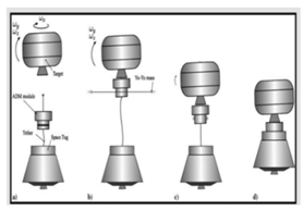 | Attaching an auxiliary device to the target through the service satellite and using the auxiliary device to eliminate the target rotation. The service satellite can avoid contact with the target, and the detumbling mode can flexibly adopt various means according to the target situation. However, similar to the above, the detumbling mode needs to be an additional device that is dedicated to the service satellite and has certain maneuverability and controllability which increases the system complexity. |
| Electrostatic [12,13,14,15] | 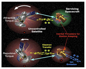 | Electrons are continuously emitted to the target through an electron-emitting device carried on the service satellite, charging the target. By doing this, the target rotation is detumbled by Coulomb electrostatic force generated by the voltage difference between the service satellite and the target. This also avoids contact between the service satellite and target. However, in this method, it is necessary to continuously charge and discharge to change the potential of the service satellite and target. In addition, this method needs to be further studied in the identification of target charge and discharge characteristics, formation maintenance and charge and discharge control algorithms. |
| Electromagnetic [16,17,18,19,20] | 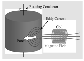 | Space debris mostly contains conductive materials such as aluminum alloys and titanium alloys. Therefore, when the target is in an external magnetic field, eddy currents are internally induced to hinder the relative motion. By using a superconducting coil to construct an external magnetic field, the target can be detumbled. The electromagnetic damping effect passively eliminates the component angular rate perpendicular to the component of the external magnetic field but does not affect the angular rate component parallel to the magnetic field direction. Thus, the relative position between the magnetic field source and the target is to be changed. In addition, the use of superconducting coils to construct a wide range of electromagnetic fields requires a corresponding power supply and cooling system. How to superimpose the superconducting magnetic field source system with service satellites requires further study. |
| Robotic Contact [21,22,23] | 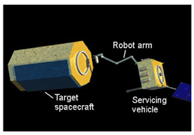 | In this method, the service satellite touches the target intermittently by using the elastic deceleration device attached to the end of the arm. The target rotation is detumbled by the friction. Robotic contact detumbling can actively adjust the direction, size and time of the control force and provide a higher braking efficiency with an accurate torque control model. However, this type of detumbling mode needs a service satellite to perform a complex orbit maneuver before implementation, located at a position very close to the target, and the collision risk is also increased. In addition, it is suitable for a target with a lower speed considering the on-orbit identification efficiency and the manipulator control precision. |
| Net or Tether [24,25,26,27,28] | 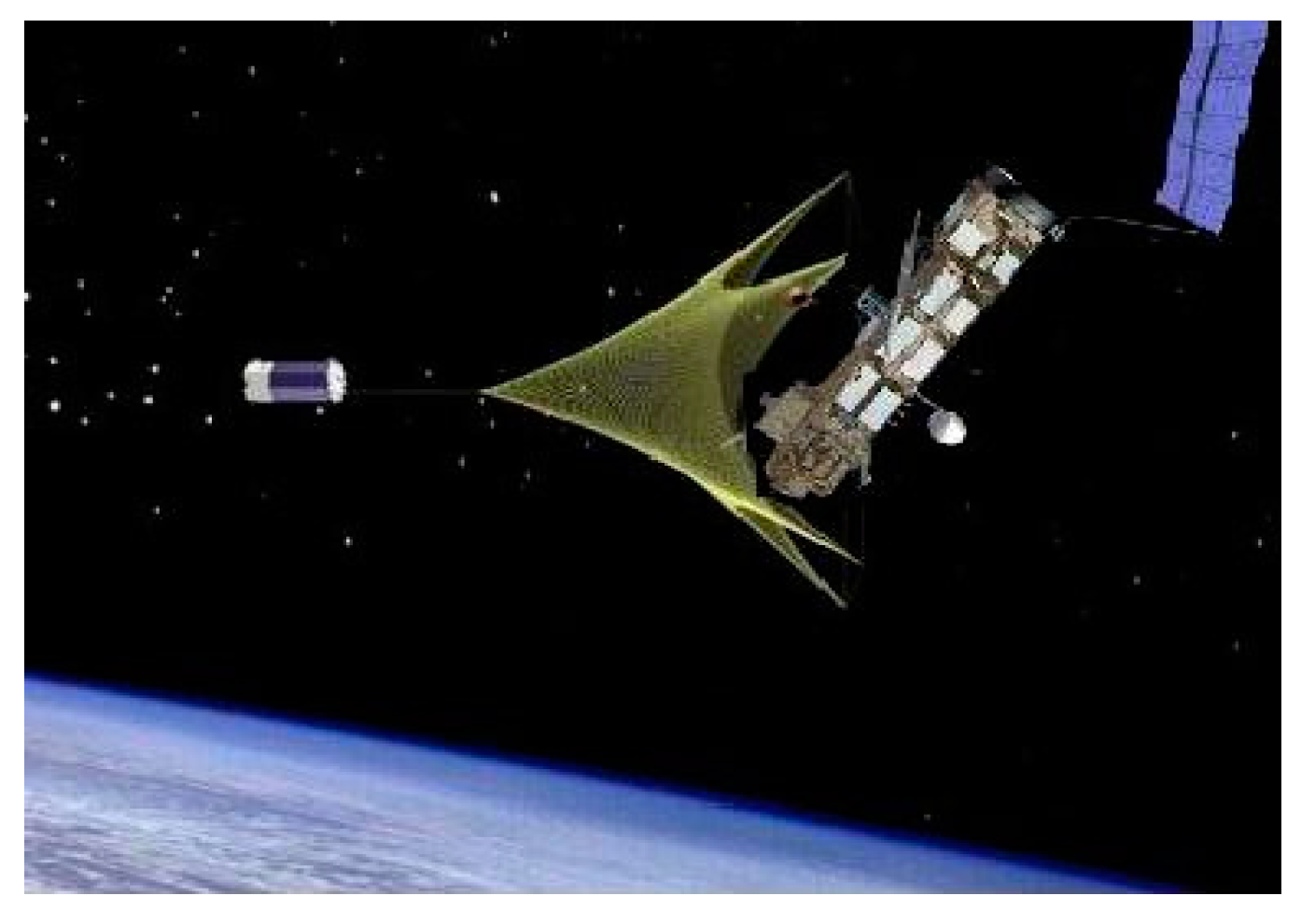 | When the net or tether catches the target, the target rotational speed is reduced by the tension and damping force of the tether. This method is only used for debris. In addition, how to avoid failure in catching and preventing the entanglement of the rope also needs further research. |
| Joint | ai | αi | di | θi |
|---|---|---|---|---|
| 0 | 0 | 0 | d0 | 0 |
| 1 | 0 | 90° | 0 | θ1 * |
| 2 | L1 | 0 | 0 | θ2 * |
| 3 | L2 | 0 | 0 | θ3 * |
| 4 | 0 | 90° | 0 | θ4 * |
| 5 | 0 | 90° | 0 | θ5 * |
| 6 | 0 | 0 | d6 | θ6 * |
| 7 | 0 | 0 | d7 * | 0 |
| 8 | a8 * | 0 | 0 | 0 |
| 1: | given initial state Θinitial, Θgoal, task time Tplan, sampling point number N, maximum angular velocity ωmax and maximum angular acceleration |
| 2: | Calculating single step response time Δt by using (23) |
| 3: | The state space is sampled by means of Halton sampling method, and the set of sampling points ΘS is obtained. |
| 4: | The path trees {Stree, Scheck, Scut} and {S’tree, S’check, S’cut} which are based on Θinitial and Θgoal is generated |
| -- | While Do |
| 5: | Finding the intersection Smeet of Stree and S’tree |
| 6: | Smeet is not empty |
| 7: | Calculate the path cost J of each point |
| 8: | Find the sampling point θmeet with the smallest J |
| 9: | By connecting Stree and S’tree with θmeet as the connection point, the path between Θinitial and Θgoal is obtained |
| 10: | Smeet is empty |
| 11: | performing FMT*algorithms on {Stree, Scheck, Scut} and {S’tree, S’check, S’cut}, respectively, and updating Stree and S’tree |
| -- | While Done |
| 12: | The local cubic polynomial interpolation is used to generate trajectory between sampling points in path |
| Type | Subtype | Value |
|---|---|---|
| Satellite platform | Central body | |
| Solar panel | ||
| Robot arm | Joint1, Joint4~6 | |
| Joint2~3 | ||
| Flexible brush | Flexible brush | |
| Simulation parameters | Initial joint state | |
| Joint torque |
| Joint | ai | αi | di | θi |
|---|---|---|---|---|
| 0 | 0 | 0 | 0.95 | 0 |
| 1 | 0 | 90° | 0 | 90° |
| 2 | 1 | 0 | 0 | 0 |
| 3 | 1 | 0 | 0 | 0 |
| 4 | 0 | 90° | 0 | 90° |
| 5 | 0 | 90° | 0 | 90° |
| 6 | 0 | 0 | 0 | 0 |
| 7 | 0 | 0 | 0.75 | 0 |
| 8 | 0 | 0 | 0 | 0 |
Publisher’s Note: MDPI stays neutral with regard to jurisdictional claims in published maps and institutional affiliations. |
© 2021 by the authors. Licensee MDPI, Basel, Switzerland. This article is an open access article distributed under the terms and conditions of the Creative Commons Attribution (CC BY) license (https://creativecommons.org/licenses/by/4.0/).
Share and Cite
Chen, N.; Zhang, Y.; Cheng, W. Space Detumbling Robot Arm Deployment Path Planning Based on Bi-FMT* Algorithm. Micromachines 2021, 12, 1231. https://doi.org/10.3390/mi12101231
Chen N, Zhang Y, Cheng W. Space Detumbling Robot Arm Deployment Path Planning Based on Bi-FMT* Algorithm. Micromachines. 2021; 12(10):1231. https://doi.org/10.3390/mi12101231
Chicago/Turabian StyleChen, Ning, Yasheng Zhang, and Wenhua Cheng. 2021. "Space Detumbling Robot Arm Deployment Path Planning Based on Bi-FMT* Algorithm" Micromachines 12, no. 10: 1231. https://doi.org/10.3390/mi12101231
APA StyleChen, N., Zhang, Y., & Cheng, W. (2021). Space Detumbling Robot Arm Deployment Path Planning Based on Bi-FMT* Algorithm. Micromachines, 12(10), 1231. https://doi.org/10.3390/mi12101231