Elastic Turbulence of Aqueous Polymer Solution in Multi-Stream Micro-Channel Flow


Abstract
:1. Introduction
2. Materials and Methods
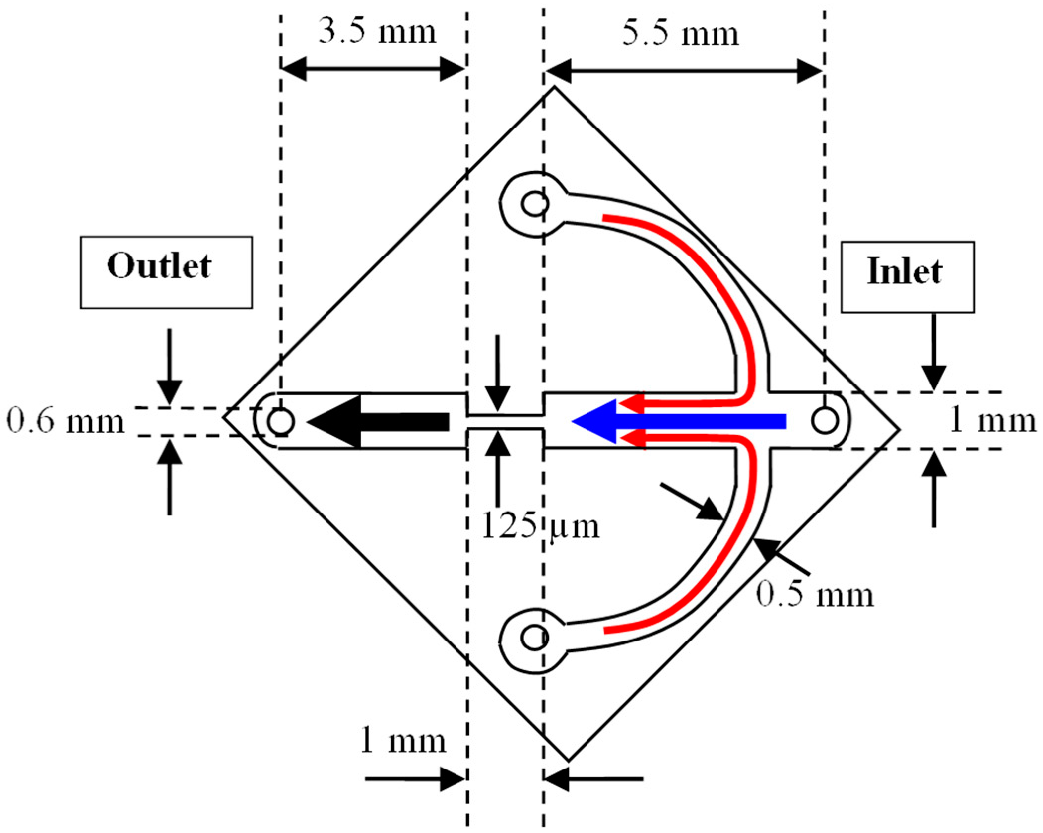
2.1. Micro-Channel
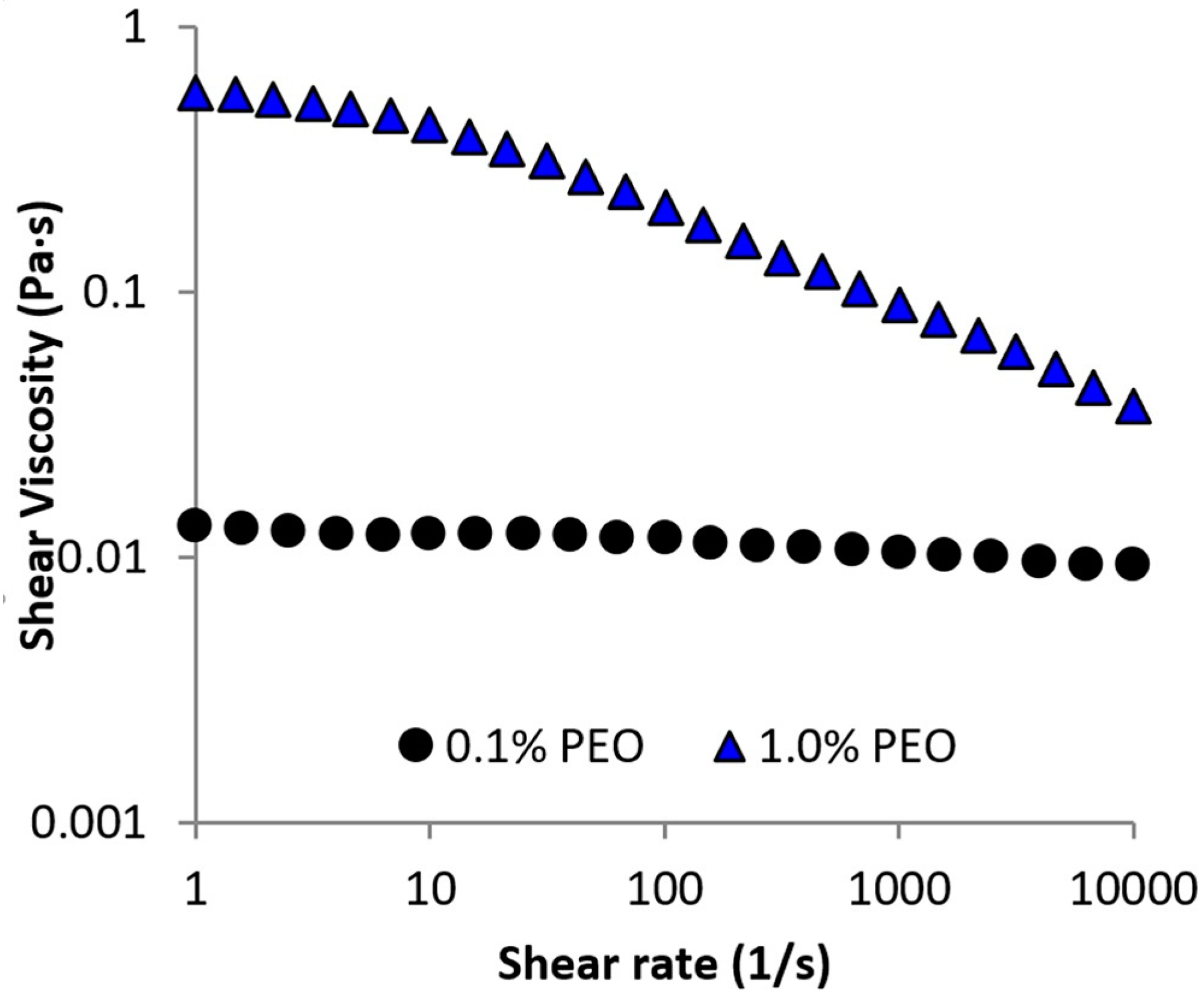
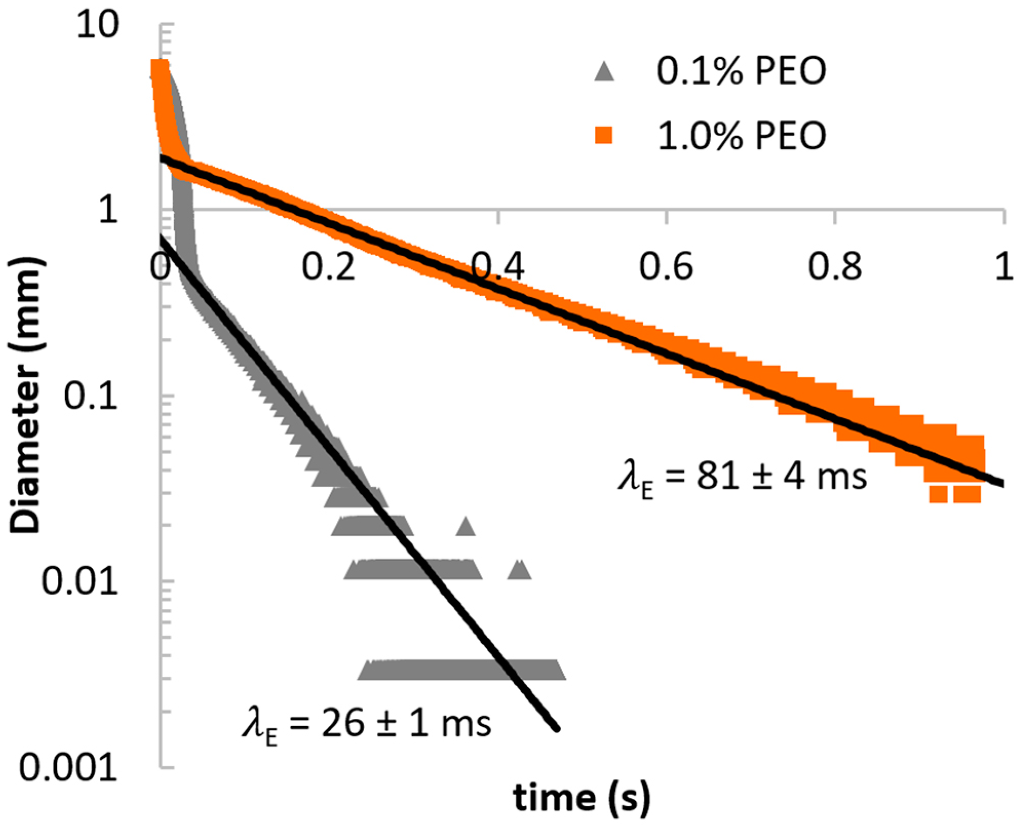
2.2. Test Liquids
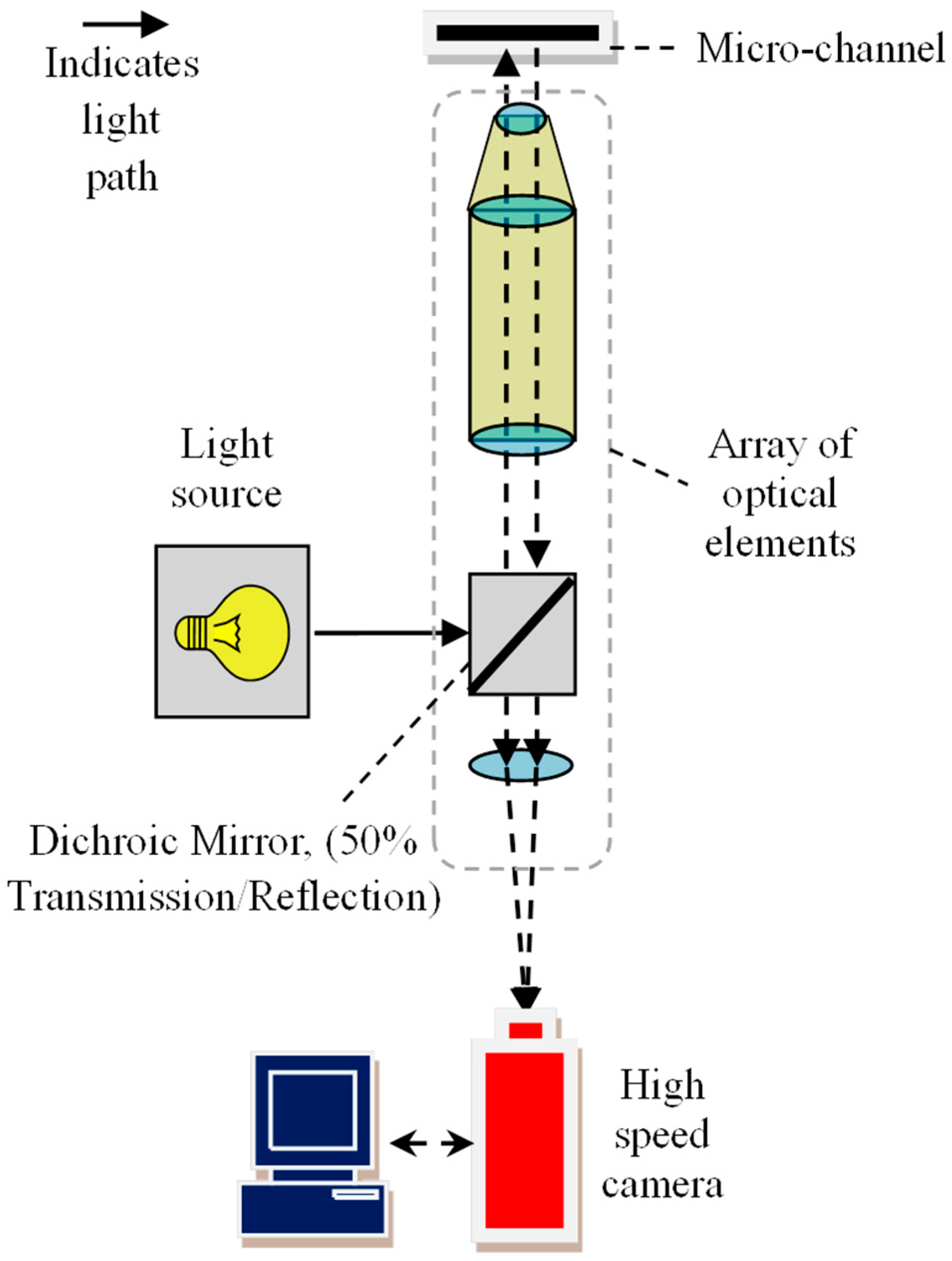
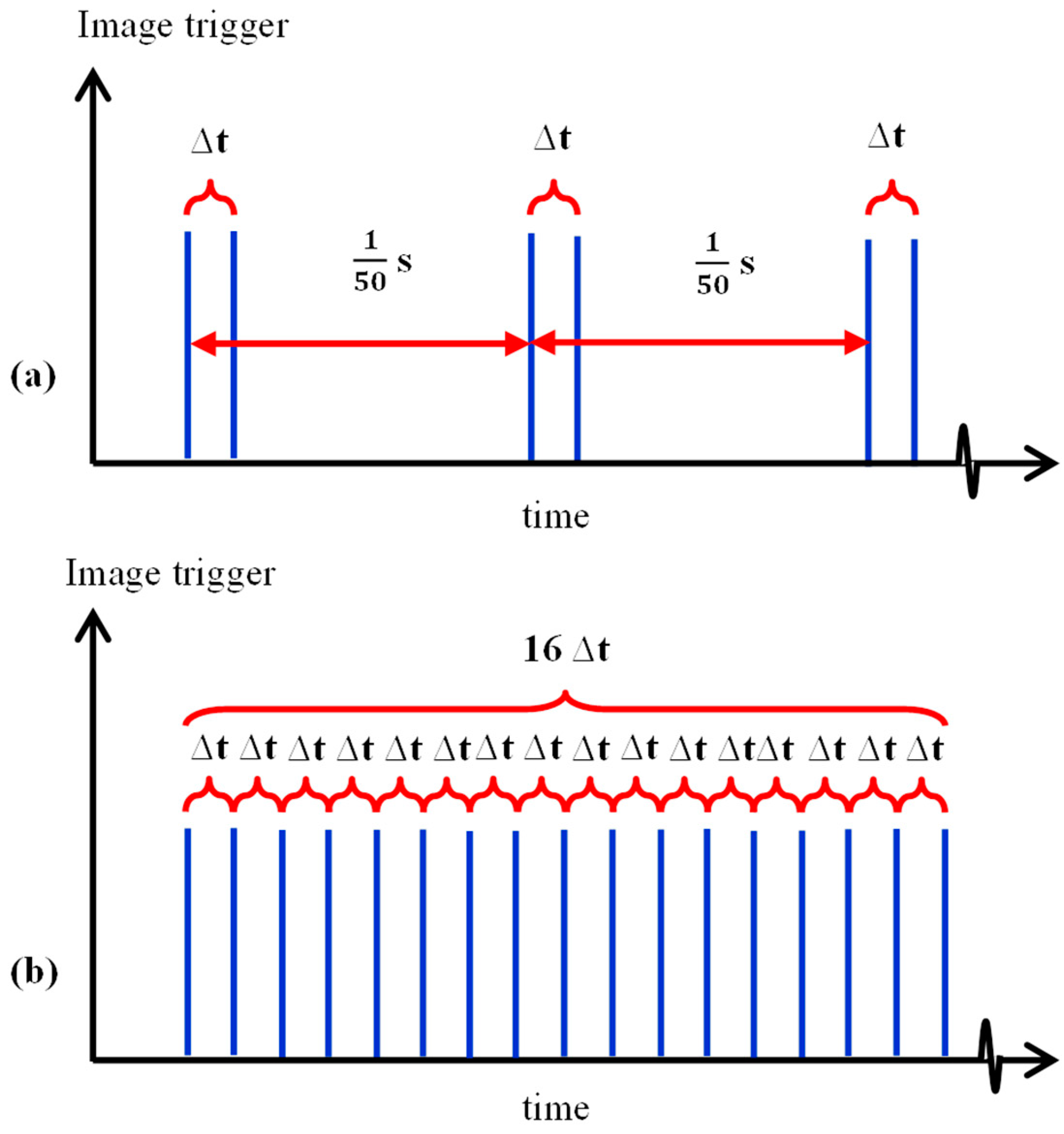
2.3. Optical Setup
3. Results and Discussion
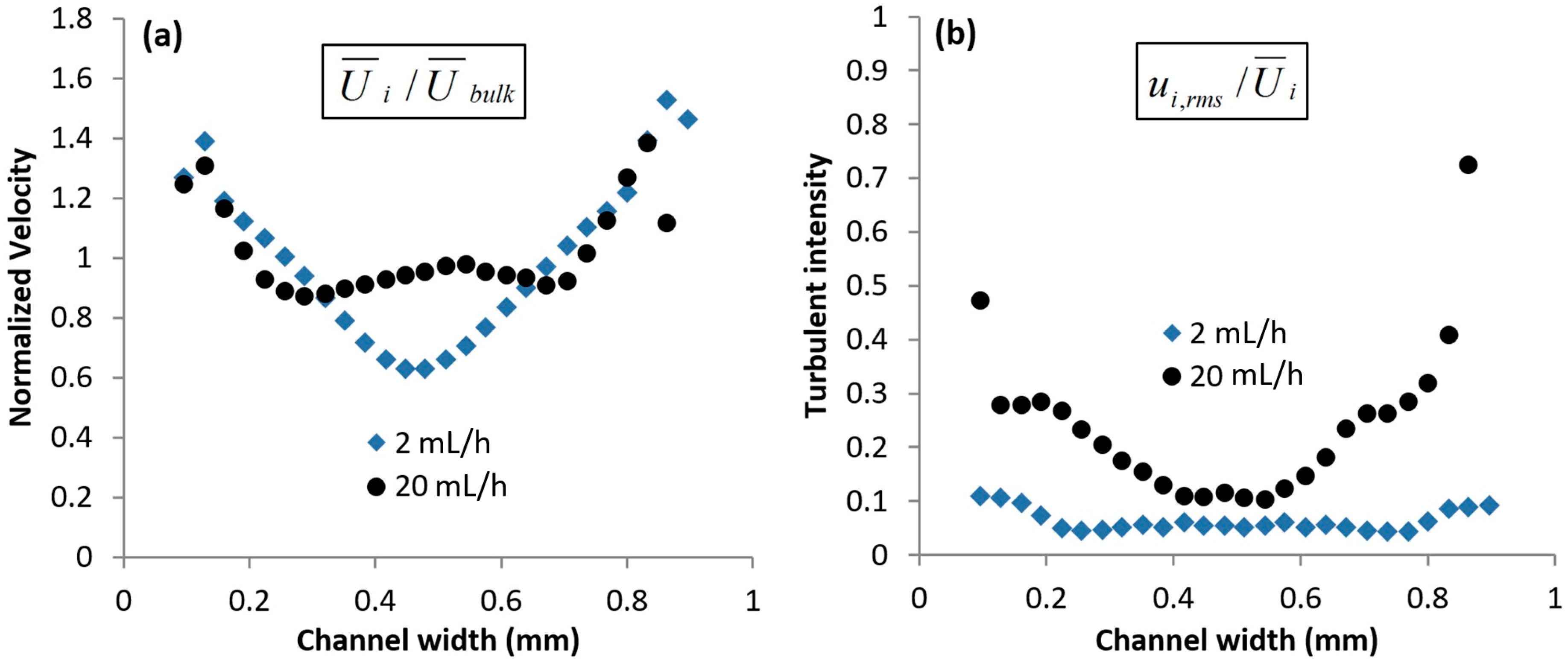
3.1. Mean Flow Statistics
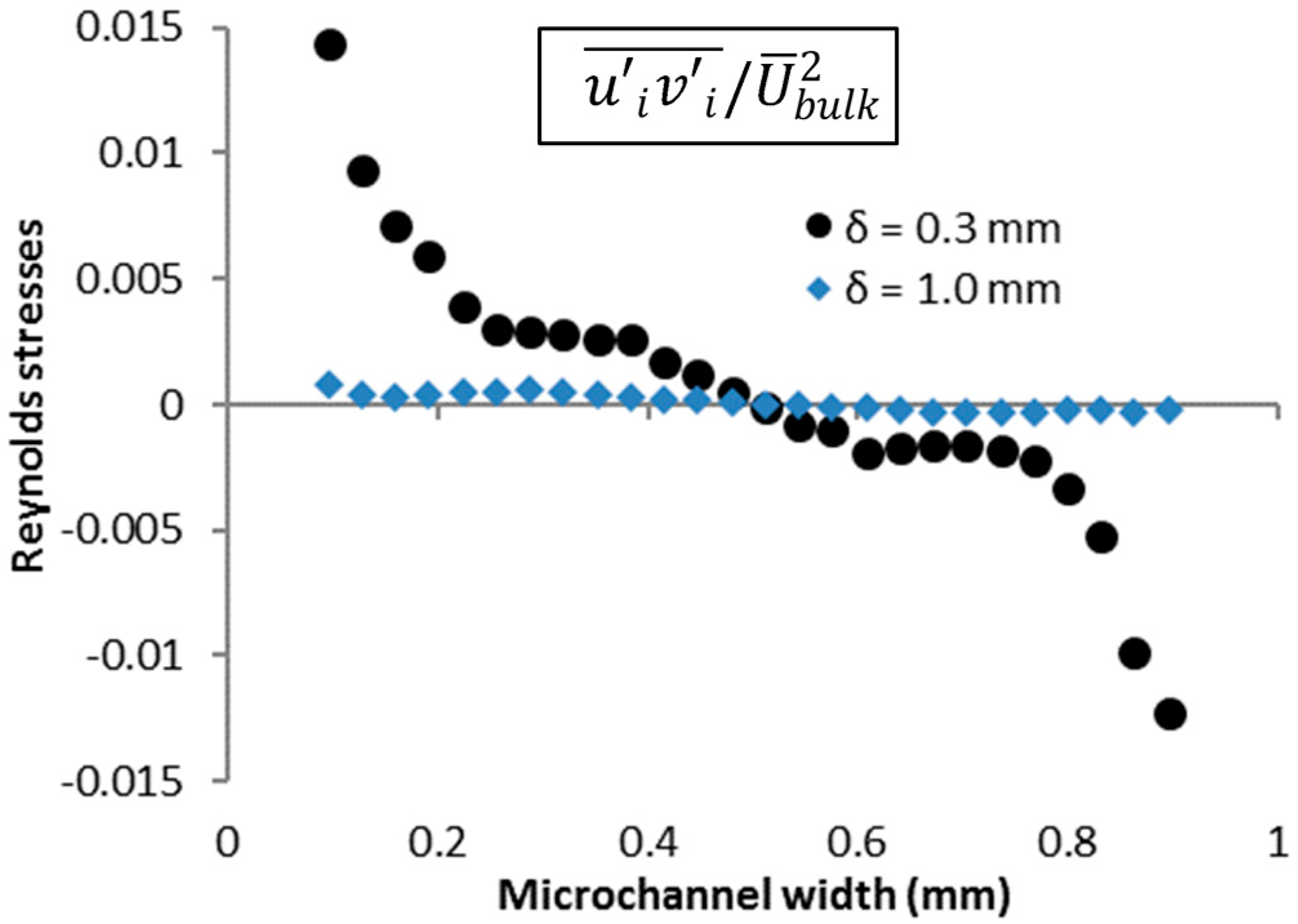
3.2. Normalized Reynolds Stresses
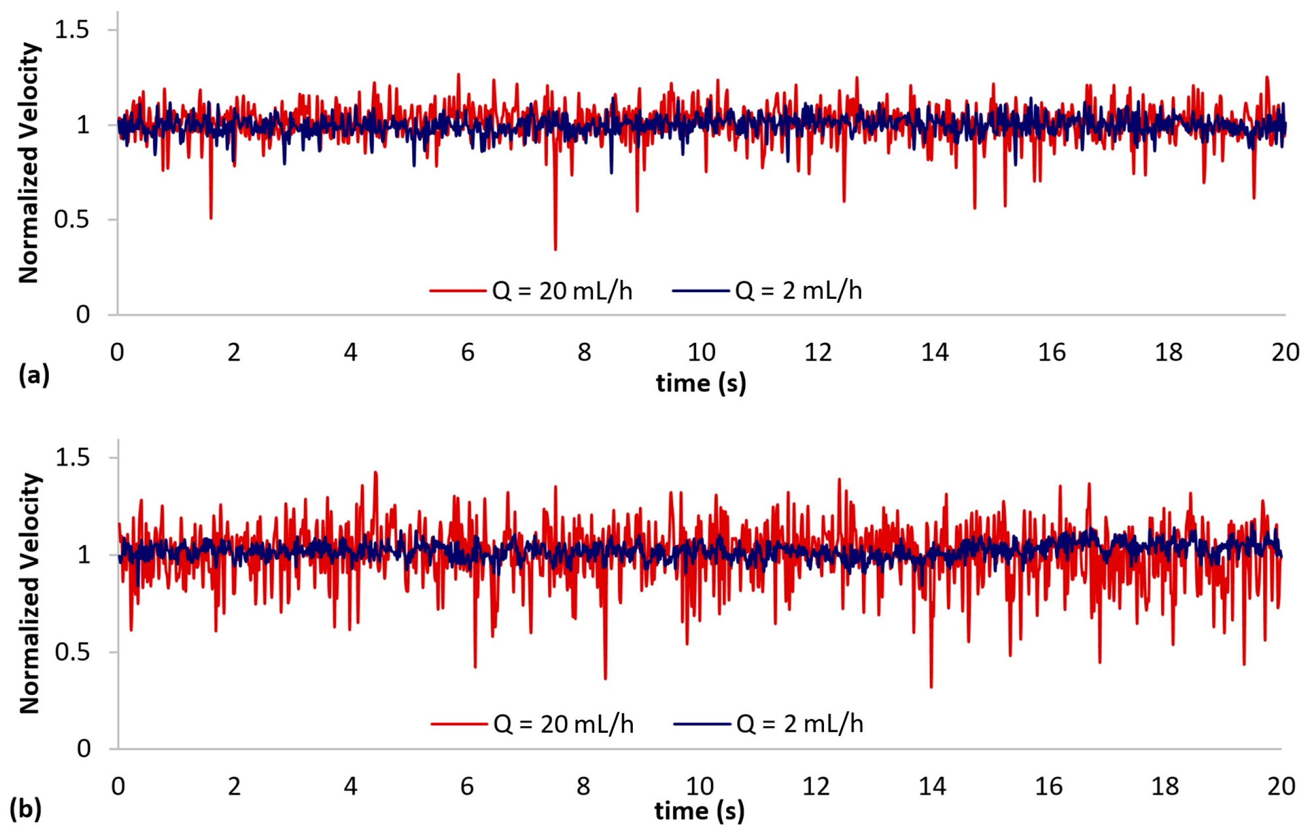
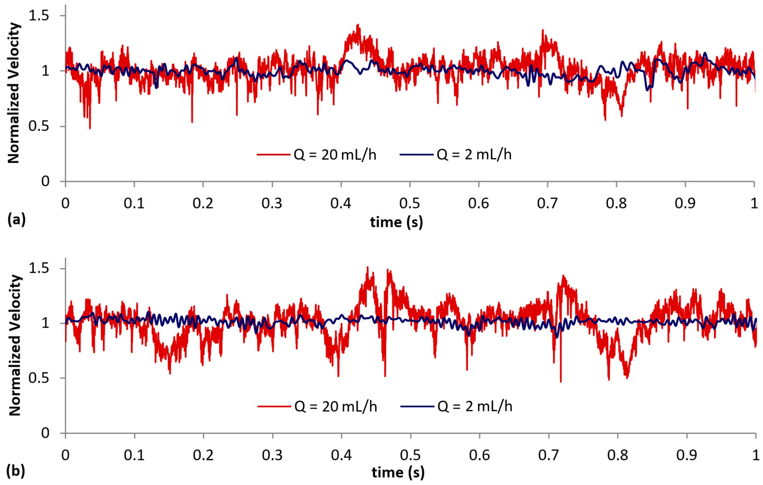
3.3. Single-Point Flow Statistics
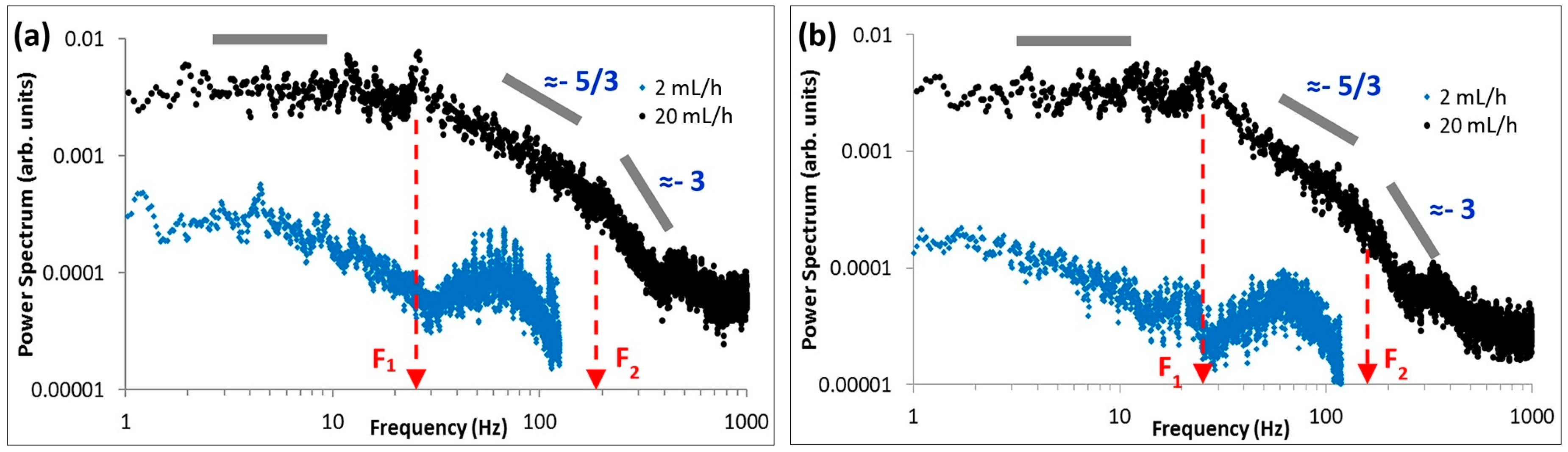
3.4. Velocity Power Spectra
3.5. Flow Field Visualization
4. Conclusions
Supplementary Materials
Author Contributions
Funding
Acknowledgments
Conflicts of Interest
References
- Tai, J.; Lim, C.P.; Lam, Y.C. Visualization of polymer relaxation in viscoelastic turbulent micro-channel flow. Sci. Rep. 2016, 5, 16633. [Google Scholar] [CrossRef] [PubMed]
- Vinogradov, G.V.; Ivanova, L.I. Wall slippage and elastic turbulence of polymers in the rubbery state. Rheol. Acta 1968, 7, 243–254. [Google Scholar] [CrossRef]
- Giesekus, H. On instabilities in Poiseuille and Couette flows of viscoelastic fluids. Prog. Heat Mass Transf. 1972, 5, 187–193. [Google Scholar]
- Groisman, A.; Steinberg, V. Elastic turbulence in a polymer solution flow. Nature 2000, 405, 53–55. [Google Scholar] [CrossRef] [PubMed]
- Groisman, A.; Steinberg, V. Stretching of polymers in a random three-dimensional flow. Phys. Rev. Lett. 2001, 86, 934. [Google Scholar] [CrossRef] [PubMed]
- Liu, Y.; Steinberg, V. Molecular sensor of elastic stress in a random flow. EPL 2010, 90, 44002. [Google Scholar] [CrossRef]
- Groisman, A.; Steinberg, V. Elastic turbulence in curvilinear flows of polymer solutions. New J. Phys. 2004, 6, 29. [Google Scholar] [CrossRef]
- Latrache, N.; Crumeyrolle, O.; Abcha, N.; Mutabazi, I. Destabilization of inertio-elastic mode via spatiotemporal intermittency in a Couette-Taylor viscoelastic flow. JPCS 2008, 137, 012022. [Google Scholar] [CrossRef]
- Dutcher, C.S.; Muller, S.J. Effects of moderate elasticity on the stability of co-and counter-rotating Taylor–Couette flows. J. Rheol. 2013, 57, 791–812. [Google Scholar] [CrossRef]
- Arratia, P.E.; Thomas, C.C.; Diorio, J.; Gollub, J.P. Elastic instabilities of polymer solutions in cross-channel flow. Phys. Rev. Lett. 2006, 96, 144502. [Google Scholar] [CrossRef]
- Haward, S.J.; Ober, T.J.; Oliveira, M.S.; Alves, M.A.; McKinley, G.H. Extensional rheology and elastic instabilities of a wormlike micellar solution in a microfluidic cross-slot device. Soft Matter 2012, 8, 536–555. [Google Scholar] [CrossRef]
- Groisman, A.; Steinberg, V. Efficient mixing at low Reynolds numbers using polymer additives. Nature 2001, 410, 905–908. [Google Scholar] [CrossRef] [PubMed]
- Burghelea, T.; Segre, E.; Bar-Joseph, I.; Groisman, A.; Steinberg, V. Chaotic flow and efficient mixing in a microchannel with a polymer solution. Phys. Rev. E 2004, 69, 066305. [Google Scholar] [CrossRef] [PubMed]
- Jun, Y.; Steinberg, V. Elastic turbulence in a curvilinear channel flow. Phys. Rev. E 2011, 84, 056325. [Google Scholar] [CrossRef] [PubMed]
- Tatsumi, K.; Takeda, Y.; Suga, K.; Nakabe, K. Turbulence characteristics and mixing performances of viscoelastic fluid flow in a serpentine microchannel. JPCS 2011, 318, 092020. [Google Scholar] [CrossRef]
- Rodd, L.E.; Scott, T.P.; Boger, D.V.; Cooper-White, J.J.; McKinley, G.H. The inertio-elastic planar entry flow of low-viscosity elastic fluids in micro-fabricated geometries. J. Nonnewton. Fluid Mech. 2005, 129, 1–22. [Google Scholar] [CrossRef]
- Rodd, L.E.; Cooper-White, J.J.; Boger, D.V.; McKinley, G.H. Role of the elasticity number in the entry flow of dilute polymer solutions in micro-fabricated contraction geometries. J. Nonnewton. Fluid Mech. 2007, 143, 170–191. [Google Scholar] [CrossRef]
- Gan, H.Y.; Lam, Y.C.; Nguyen, N.T.; Tam, K.C.; Yang, C. Efficient mixing of viscoelastic fluids in a microchannel at low Reynolds number. Microfluid. Nanofluid. 2007, 3, 101–108. [Google Scholar] [CrossRef]
- Lam, Y.C.; Gan, H.Y.; Nguyen, N.T.; Lie, H. Micromixer based on viscoelastic flow instability at low Reynolds number. Biomicrofluidics 2009, 3, 014106. [Google Scholar] [CrossRef]
- Rodd, L.E.; Lee, D.; Ahn, K.H.; Cooper-White, J.J. The importance of downstream events in microfluidic viscoelastic entry flows: Consequences of increasing the constriction length. J. Nonnewton. Fluid Mech. 2010, 165, 1189–1203. [Google Scholar] [CrossRef]
- Bonn, D.; Ingremeau, F.; Amarouchene, Y.; Kellay, H. Large velocity fluctuations in small-Reynolds-number pipe flow of polymer solutions. Phys. Rev. E 2011, 84, 045301. [Google Scholar] [CrossRef] [PubMed]
- Gan, H.Y.; Lam, Y.C. Experimental observations of flow instabilities and rapid mixing of two dissimilar viscoelastic liquids. AIP Adv. 2012, 2, 042146. [Google Scholar] [CrossRef]
- Li, F.C.; Kinoshita, H.; Li, X.B.; Oishi, M.; Fujii, T.; Oshima, M. Creation of very-low-Reynolds-number chaotic fluid motions in microchannels using viscoelastic surfactant solution. Exp. Therm. Fluid Sci. 2010, 34, 20–27. [Google Scholar] [CrossRef]
- Grilli, M.; Vázquez-Quesada, A.; Ellero, M. Transition to turbulence and mixing in a viscoelastic fluid flowing inside a channel with a periodic array of cylindrical obstacles. Phys. Rev. Lett. 2013, 110, 174501. [Google Scholar] [CrossRef] [PubMed]
- White, J.L.; Kondo, A. Flow patterns in polyethylene and polystyrene melts during extrusion through a die entry region: Measurement and interpretation. J. Nonnewton. Fluid Mech. 1977, 3, 41–64. [Google Scholar] [CrossRef]
- Nguyen, H.; Boger, D.V. The kinematics and stability of die entry flows. J. Nonnewton. Fluid Mech. 1979, 5, 353–368. [Google Scholar] [CrossRef]
- Lawler, J.V.; Muller, S.J.; Brown, R.A.; Armstrong, R.C. Laser Doppler velocimetry measurements of velocity fields and transitions in viscoelastic fluids. J. Nonnewton. Fluid Mech. 1986, 20, 51–92. [Google Scholar] [CrossRef]
- Yesilata, B.; Öztekin, A.; Neti, S. Instabilities in viscoelastic flow through an axisymmetric sudden contraction. J. Nonnewton. Fluid Mech. 1999, 85, 35–62. [Google Scholar] [CrossRef]
- Zhang, H.N.; Li, F.C.; Cao, Y.; Kunugi, T.; Yu, B. Direct numerical simulation of elastic turbulence and its mixing-enhancement effect in a straight channel flow. Chin. Phys. B 2013, 22, 024703. [Google Scholar] [CrossRef]
- Whalley, R.D.; Abed, W.M.; Dennis, D.J.C.; Poole, R.J. Enhancing heat transfer at the micro-scale using elastic turbulence. TAML 2015, 5, 103–106. [Google Scholar] [CrossRef]
- Abed, W.M.; Whalley, R.D.; Dennis, D.J.; Poole, R.J. Experimental investigation of the impact of elastic turbulence on heat transfer in a serpentine channel. J. Nonnewton. Fluid Mech. 2016, 231, 68–78. [Google Scholar] [CrossRef]
- Ligrani, P.; Copeland, D.; Ren, C.; Su, M.; Suzuki, M. Heat transfer enhancements from elastic turbulence using sucrose-based polymer solutions. J. Thermophys. Heat Transf. 2018, 32, 51–60. [Google Scholar] [CrossRef]
- Taylor, Z.J.; Gurka, R.; Kopp, G.; Liberzon, A. Long-duration time-resolved PIV to study unsteady aerodynamics. IEEE Trans. Instrum. Meas. 2010, 59, 3262–3269. [Google Scholar] [CrossRef]
- Barnes, H.A.; Hutton, J.F.; Walters, K. An Introduction to Rheology; Elsevier: Amsterdam, The Netherlands, 1989; Volume 3, p. 62. [Google Scholar]
- Tamano, S.; Itoh, M.; Inoue, T.; Kato, K.; Yokota, K. Turbulence statistics and structures of drag-reducing turbulent boundary layer in homogeneous aqueous surfactant solutions. Phys. Fluids 2009, 21, 045101. [Google Scholar] [CrossRef]
- Japper-Jaafar, A.; Escudier, M.P.; Poole, R.J. Laminar, transitional and turbulent annular flow of drag-reducing polymer solutions. J. Nonnewton. Fluid Mech. 2010, 165, 1357–1372. [Google Scholar] [CrossRef]
- Kraichnan, R.H. Inertial ranges in two-dimensional turbulence. Phys. Fluids 1967, 10, 1417. [Google Scholar] [CrossRef]
- Leith, C.E. Diffusion approximation for two-dimensional turbulence. Phys. Fluids 1968, 11, 671–672. [Google Scholar] [CrossRef]
- Batchelor, G.K. Computation of the energy spectrum in homogeneous two-dimensional turbulence. Phys. Fluids 1969, 12, II–233. [Google Scholar] [CrossRef]
- Raffel, M.; Willert, C.; Wereley, S.; Kompenhans, J. Particle Image Velocimetry—A Practical Guide, 2nd ed.; Springer: Berlin/Heidelberg, Germany, 2007; p. 193. [Google Scholar]
- Adrian, R.J.; Christensen, K.T.; Liu, Z.C. Analysis and interpretation of instantaneous turbulent velocity fields. Exp. Fluids 2000, 29, 275–290. [Google Scholar] [CrossRef]


| Test Liquid | PEO (g) | Glycerol (g) | Water (g) | Microsphere (g) |
|---|---|---|---|---|
| Center-stream | 1.00 | 55 | 44 | 0.03 |
| Side-stream | 0.10 | 55 | 44 | 0.03 |
| Properties | Extensional Relaxation Time (ms) | Flow Rate (mL/h) | Δt (s) | Mean Velocity (, m/s) | Shear Rate (, s−1) | Viscosity (, Pa·s) | Re | De | |
|---|---|---|---|---|---|---|---|---|---|
| Fluid | |||||||||
| Center-stream Liquid | 81 ± 4 | 2 | 0.004 | 0.03 | 364 | 0.126 | 0.022 | 27 | |
| 20 | 0.00025 | 0.31 | 4262 | 0.052 | 0.528 | 278 | |||
| Side-stream Liquid | 26 ± 1 | 2 | 0.004 | 0.02 | 1107 | 0.01 | 0.145 | 6 | |
| 20 | 0.00025 | 0.21 | 10514 | 0.01 | 1.45 | 59 | |||
© 2019 by the authors. Licensee MDPI, Basel, Switzerland. This article is an open access article distributed under the terms and conditions of the Creative Commons Attribution (CC BY) license (http://creativecommons.org/licenses/by/4.0/).
Share and Cite
Tai, J.; Lam, Y.C. Elastic Turbulence of Aqueous Polymer Solution in Multi-Stream Micro-Channel Flow. Micromachines 2019, 10, 110. https://doi.org/10.3390/mi10020110
Tai J, Lam YC. Elastic Turbulence of Aqueous Polymer Solution in Multi-Stream Micro-Channel Flow. Micromachines. 2019; 10(2):110. https://doi.org/10.3390/mi10020110
Chicago/Turabian StyleTai, Jiayan, and Yee Cheong Lam. 2019. "Elastic Turbulence of Aqueous Polymer Solution in Multi-Stream Micro-Channel Flow" Micromachines 10, no. 2: 110. https://doi.org/10.3390/mi10020110
APA StyleTai, J., & Lam, Y. C. (2019). Elastic Turbulence of Aqueous Polymer Solution in Multi-Stream Micro-Channel Flow. Micromachines, 10(2), 110. https://doi.org/10.3390/mi10020110