Accelerated Particle Separation in a DLD Device at Re > 1 Investigated by Means of µPIV

 , , ,
, , ,  and
and 
Abstract
:1. Introduction
2. Materials and Methods
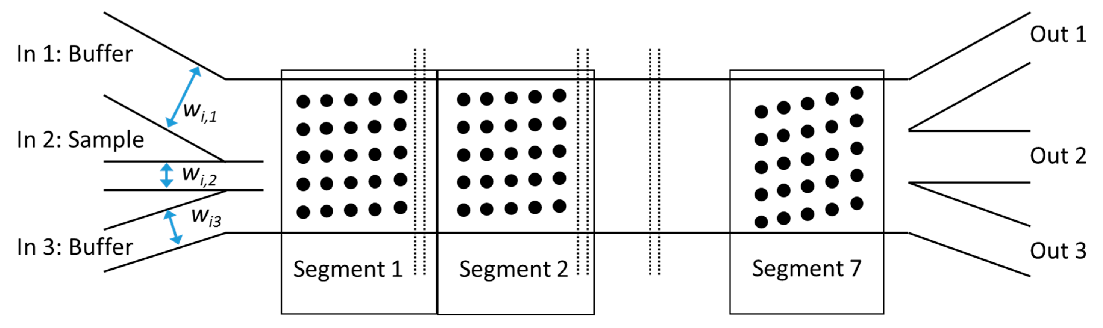
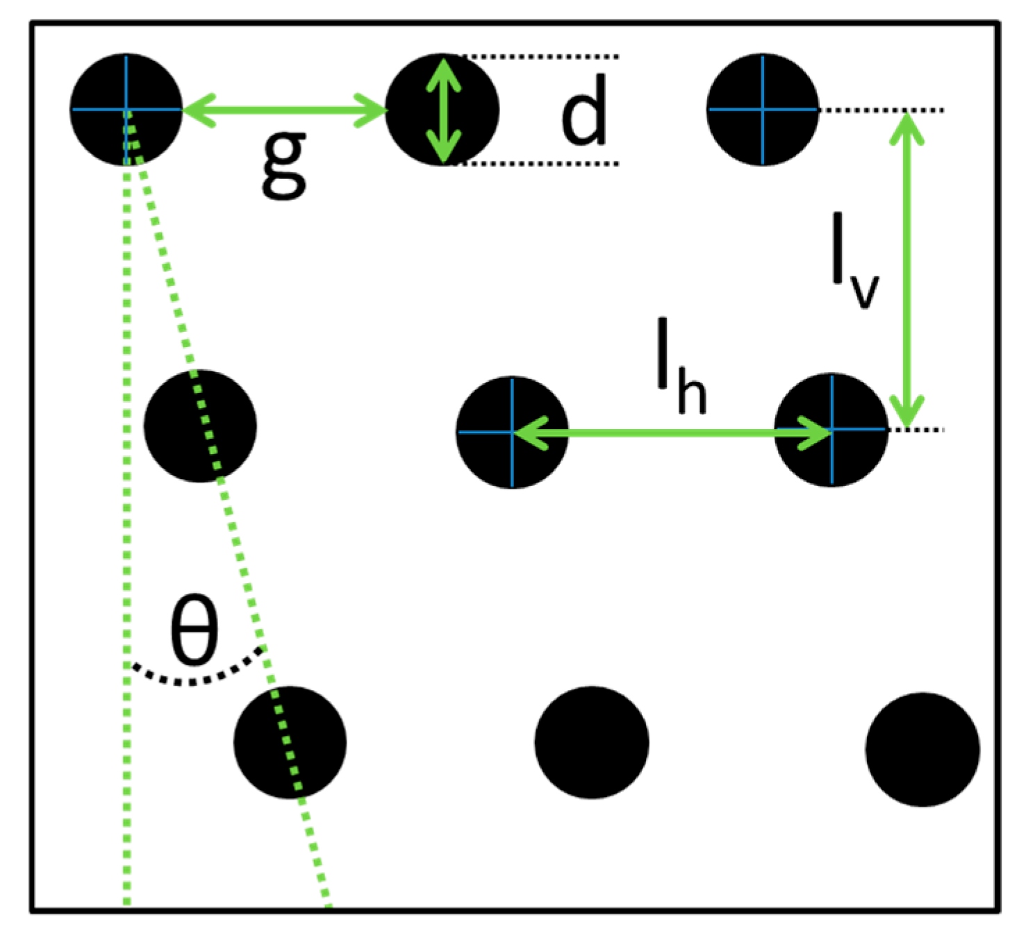
2.1. Segmented DLD Design
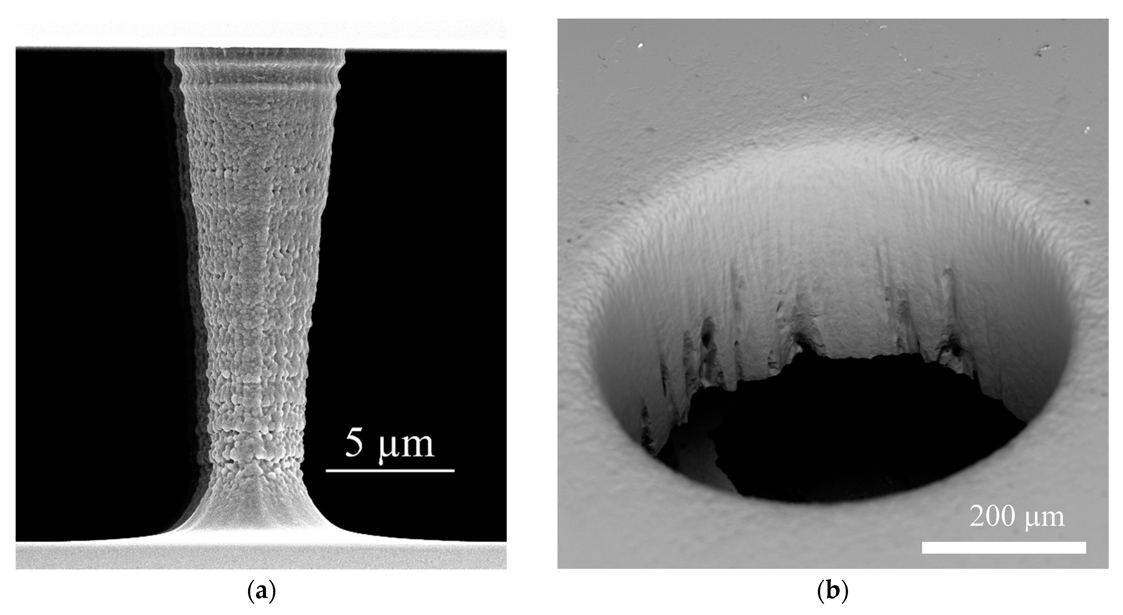
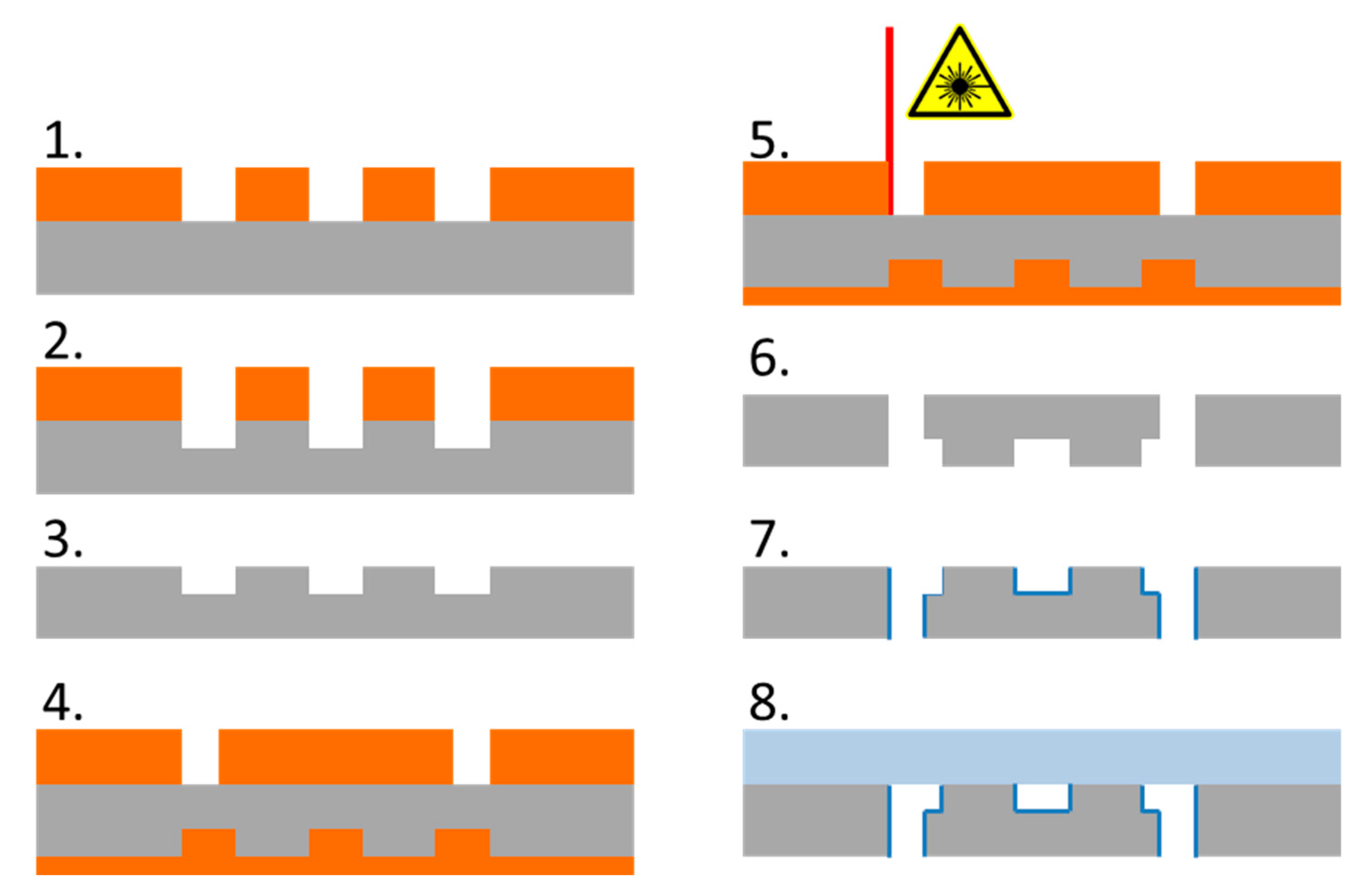
2.2. Fabrication of the DLD Devices
2.3. Flow Control Setup
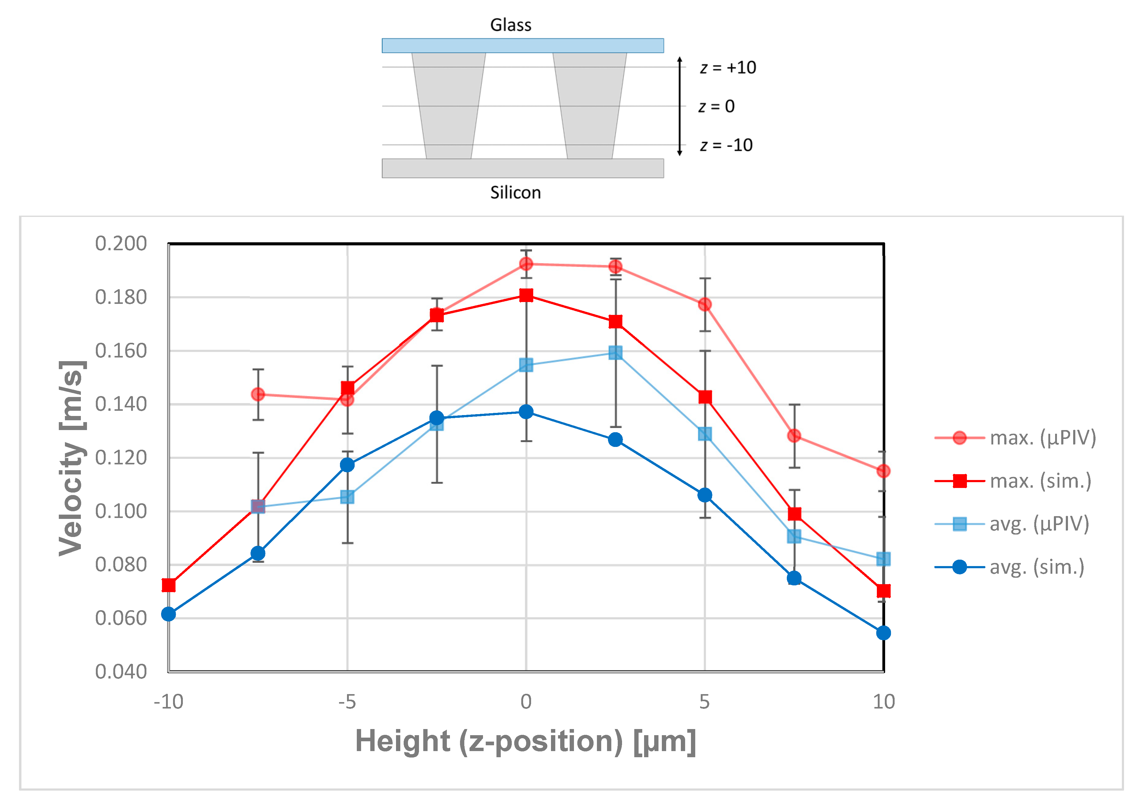
2.4. µPIV Setup
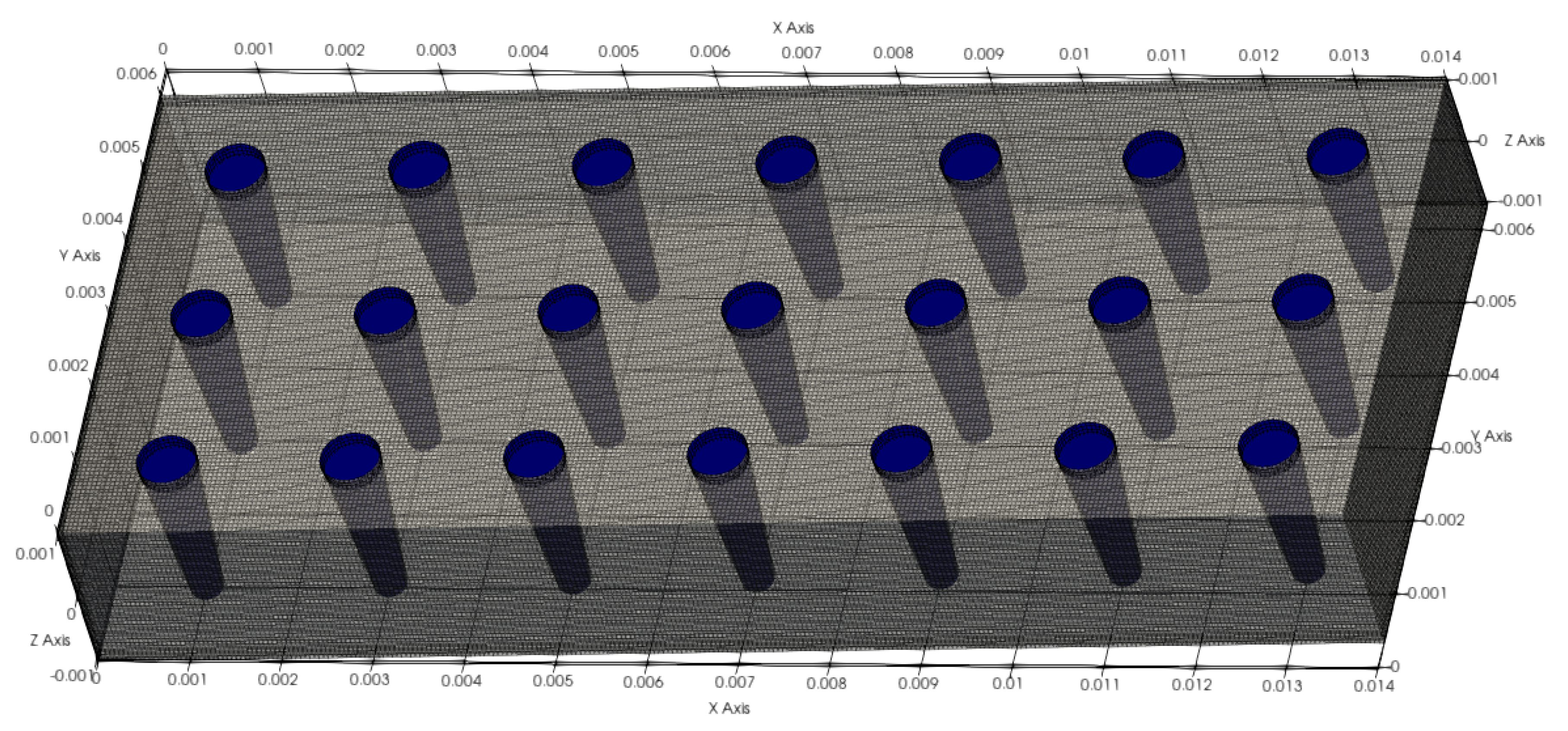
2.5. Simulation
3. Results and Discussion
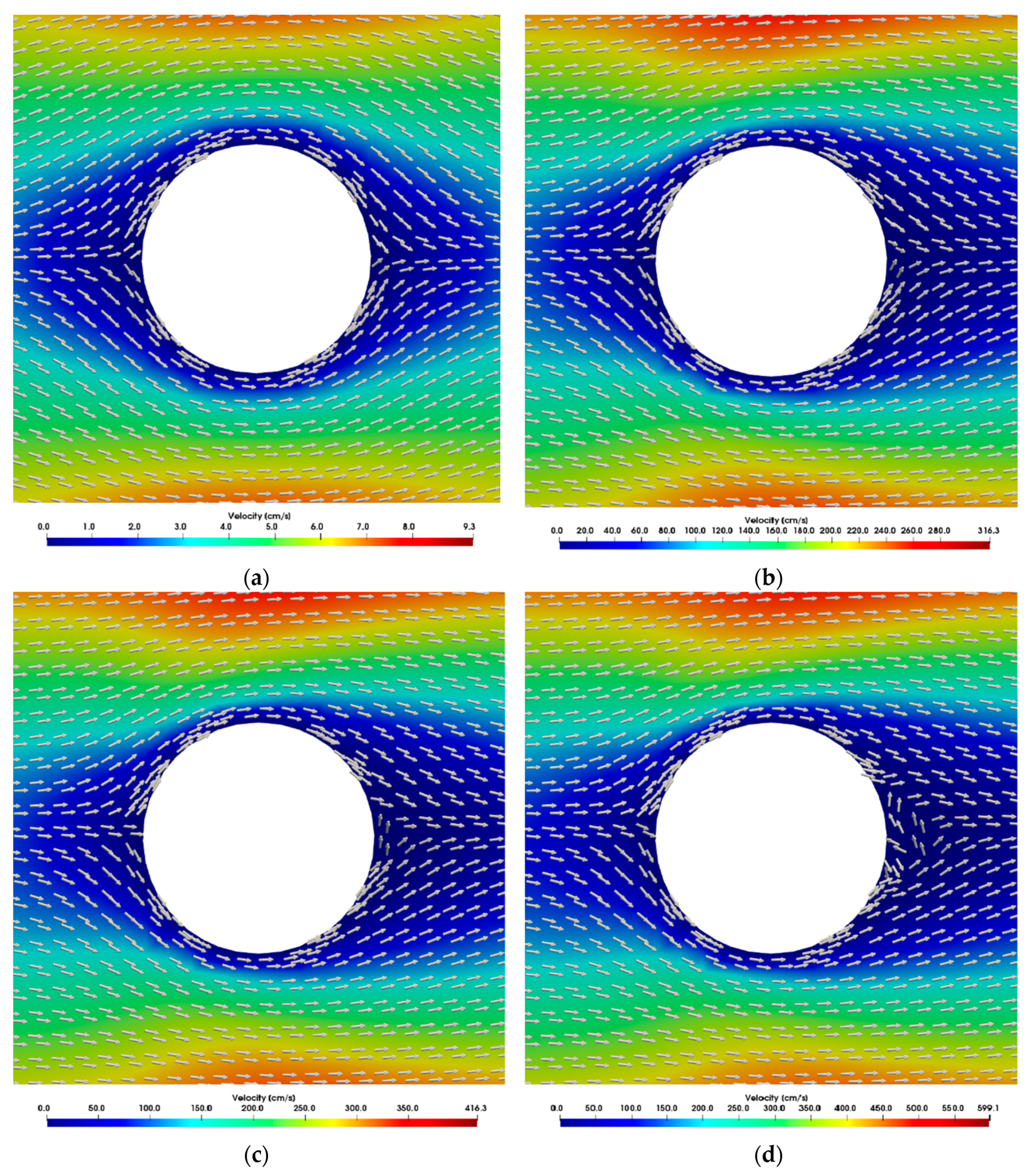
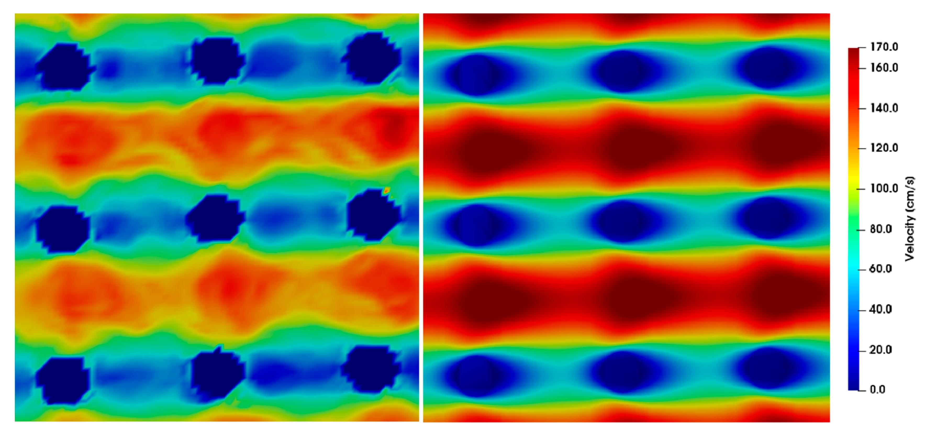
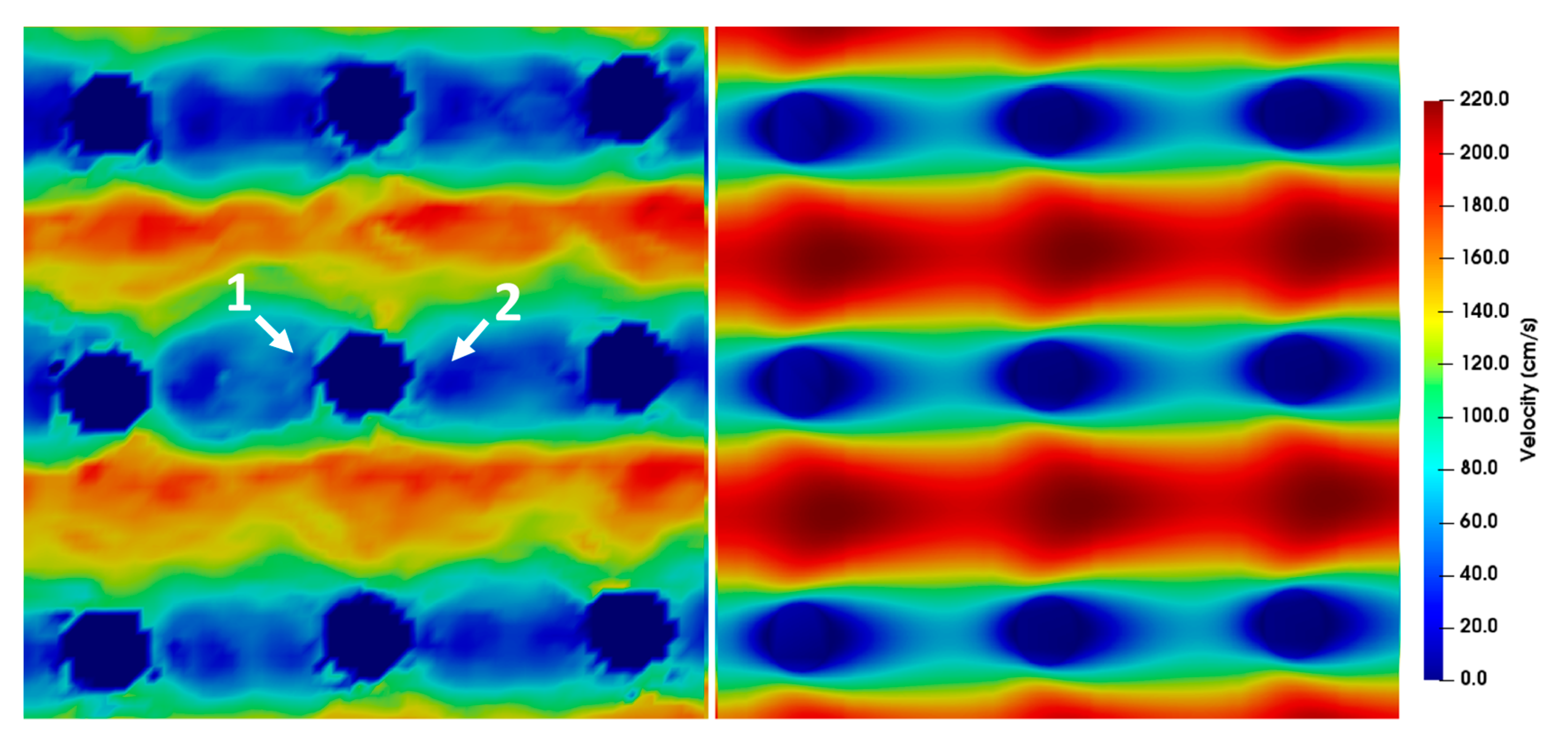
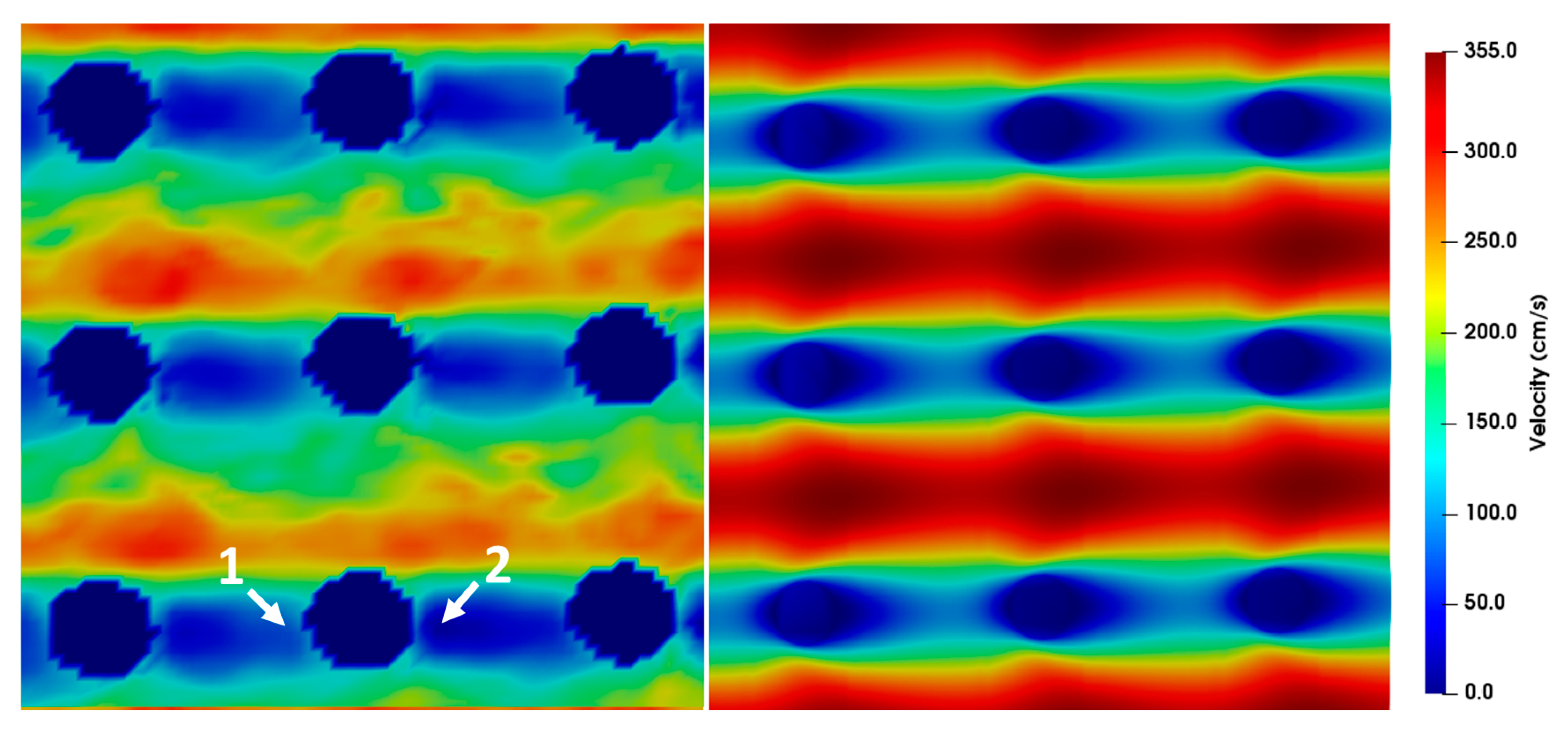
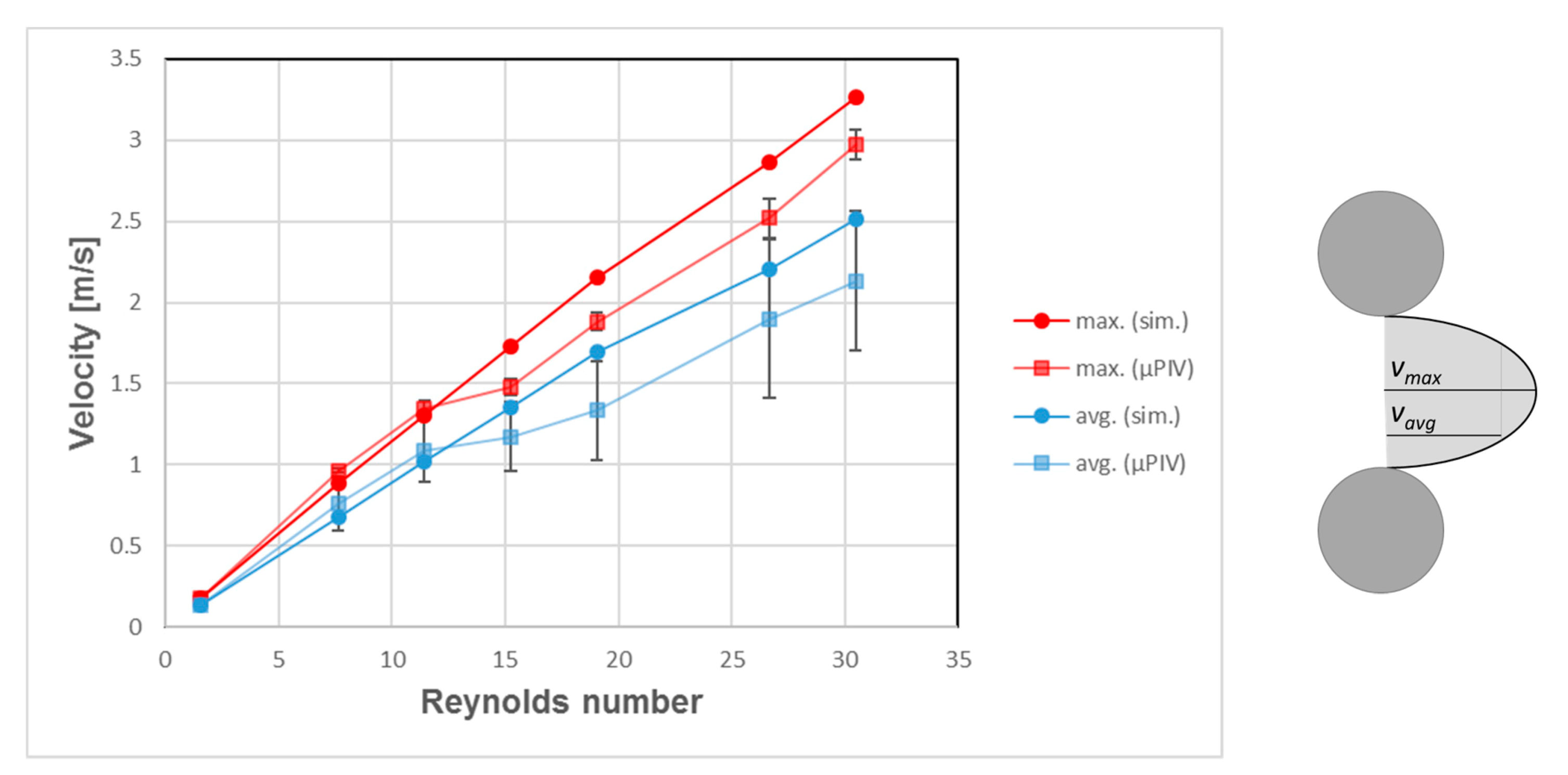
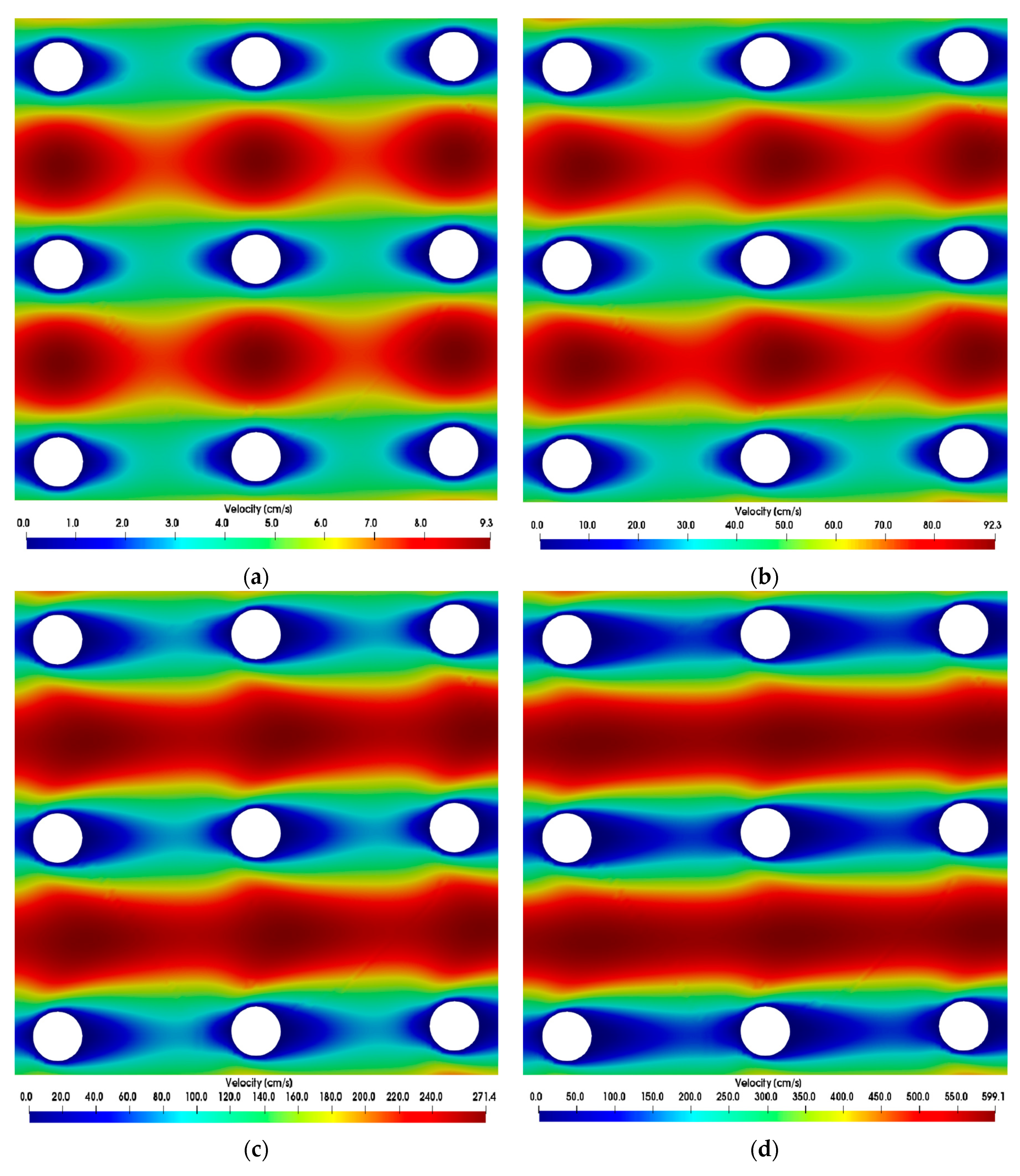
3.1. Simulations
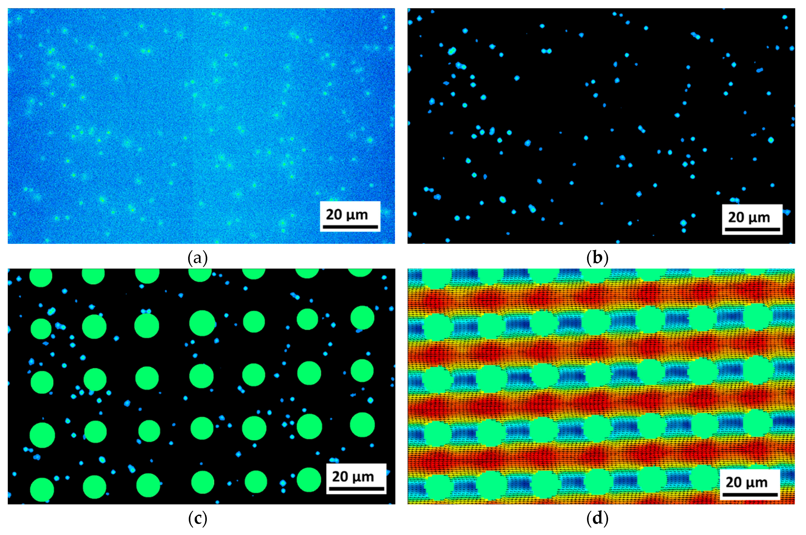
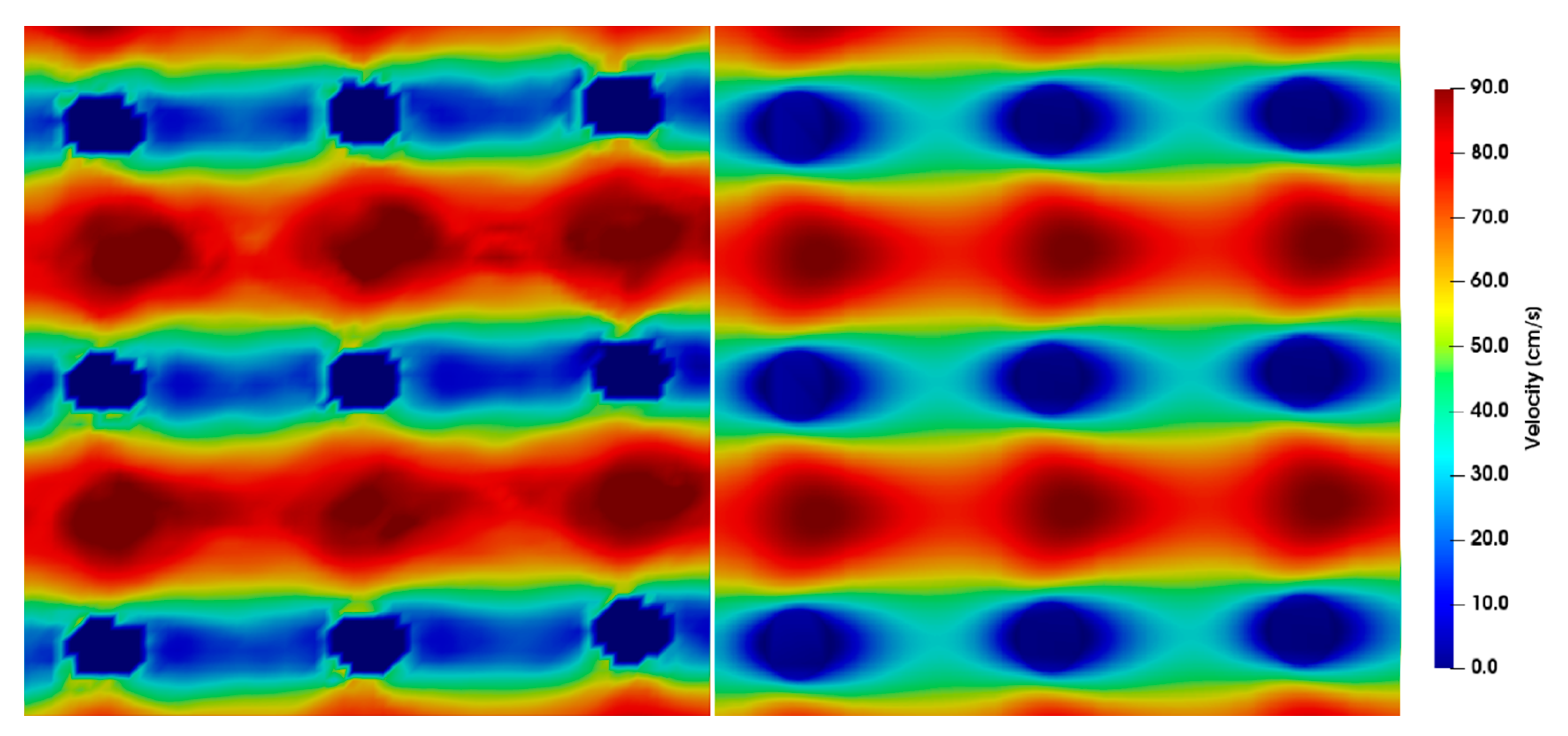
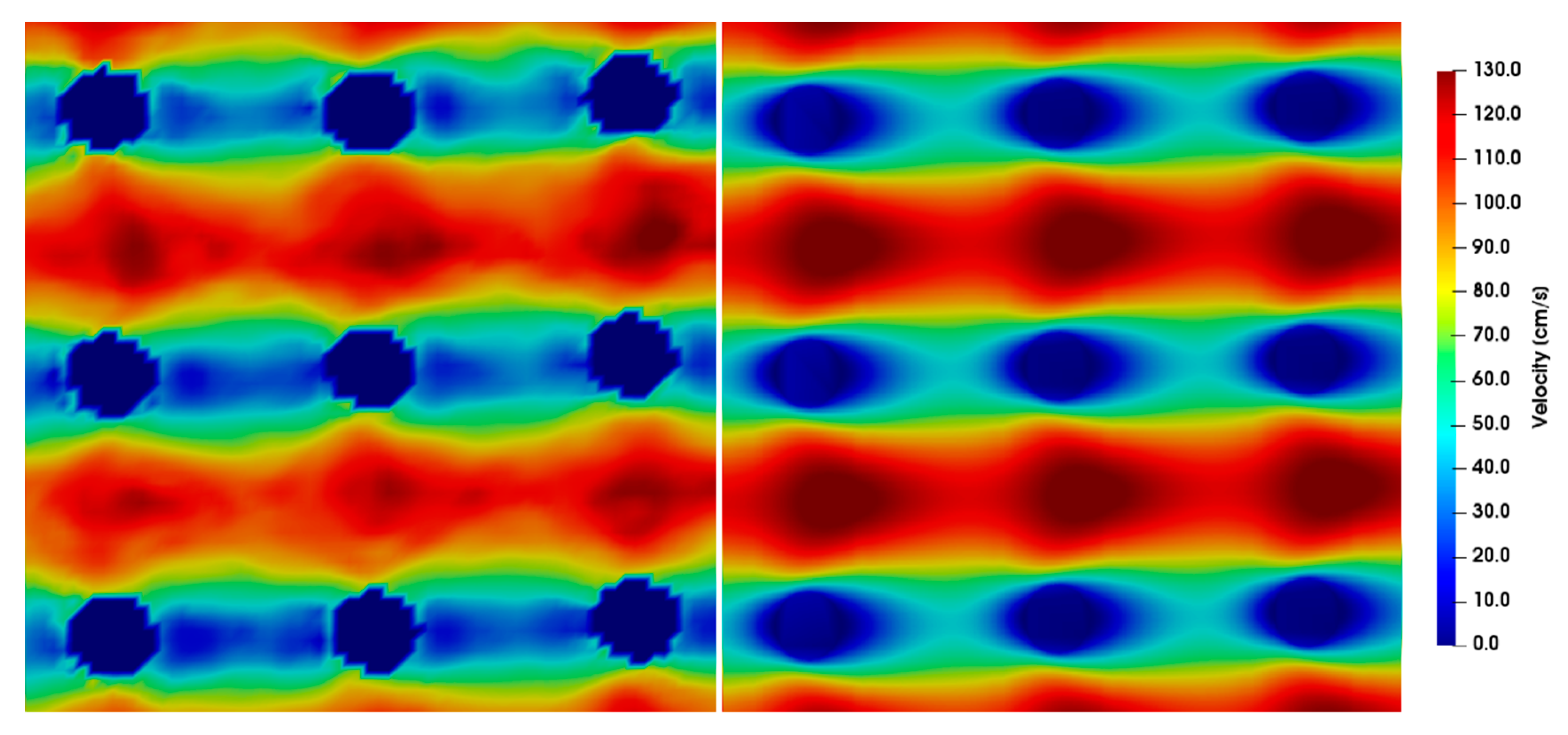
3.2. Comparison between Simulations and µPIV Results
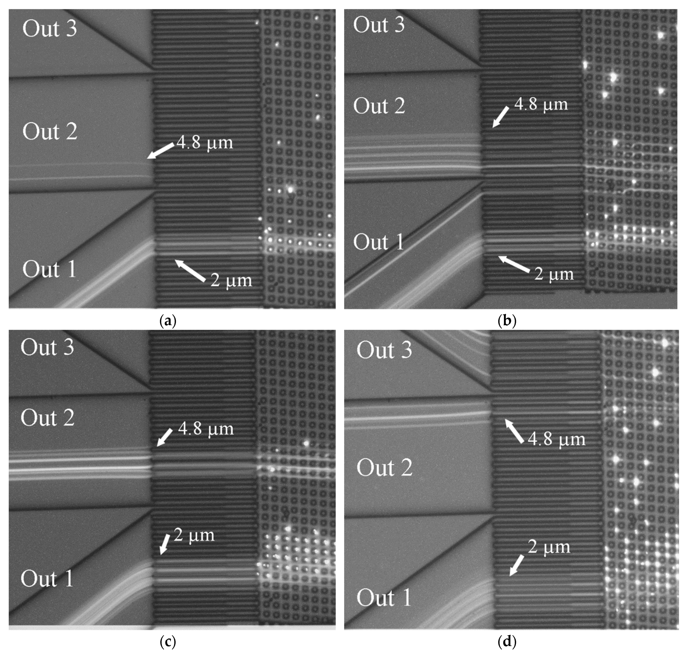
3.3. Fractionation Results
4. Conclusions and Outlook
Author Contributions
Funding
Conflicts of Interest
References
- Shekunov, B.Y.; Chattopadhyay, P.; Tong, H.H.Y.; Chow, A.H.L. Particle size analysis in pharmaceutics: Principles, methods and applications. Pharm. Res. 2007, 24, 203–227. [Google Scholar] [CrossRef] [PubMed]
- Davis, J. Microfluidic Separation of Blood Components through Deterministic Lateral Displacement. Ph.D. Thesis, Princeton University, Princeton, NJ, USA, 2008. [Google Scholar]
- Sajeesh, P.; Sen, A.K. Particle separation and sorting in microfluidic devices: A review. Microfluid Nanofluid 2014, 17, 1–52. [Google Scholar] [CrossRef]
- Albagdady, A.; Al-Faqheri, W.; Kottmeier, J.; Meinen, S.; Frey, L.J.; Krull, R.; Dietzel, A. Enhanced inertial focusing of microparticles and cells by integrating trapezoidal microchambers in spiral microfluidic channels. RSC Adv. 2019, 9, 19197–19204. [Google Scholar] [CrossRef]
- McGrath, J.; Jimenez, M.; Bridle, H. Deterministic lateral displacement for particle separation: A review. Lab Chip 2014, 14, 4139–4158. [Google Scholar] [CrossRef] [PubMed]
- Wunsch, B.H.; Smith, J.T.; Gifford, S.M.; Wang, C.; Brink, M.; Bruce, R.L.; Austin, R.H.; Stolovitzky, G.; Astier, Y. Nanoscale lateral displacement arrays for the separation of exosomes and colloids down to 20 nm. Nat. Nanotechnol. 2016, 11, 936–940. [Google Scholar] [CrossRef] [PubMed]
- Lubbersen, Y.S.; Schutyser, M.A.I.; Boom, R.M. Suspension separation with deterministic ratchets at moderate Reynolds numbers. Chem. Eng. Sci. 2012, 73, 314–320. [Google Scholar] [CrossRef]
- Lubbersen, Y.S.; Dijkshoorn, J.P.; Schutyser, M.A.I.; Boom, R.M. Visualization of inertial flow in deterministic ratchets. Sep. Purif. Technol. 2013, 109, 33–39. [Google Scholar] [CrossRef]
- Dincau, B.M.; Aghilinejad, A.; Hammersley, T.; Chen, X.; Kim, J.-H. Deterministic lateral displacement (DLD) in the high Reynolds number regime: High-throughput and dynamic separation characteristics. Microfluid Nanofluid 2018, 22, 869. [Google Scholar] [CrossRef]
- Zeming, K.K.; Thakor, N.V.; Zhang, Y.; Chen, C.-H. Real-time modulated nanoparticle separation with an ultra-large dynamic range. Lab Chip 2016, 16, 75–85. [Google Scholar] [CrossRef] [PubMed]
- Calero, V.; Garcia-Sanchez, P.; Honrado, C.; Ramos, A.; Morgan, H. AC electrokinetic biased deterministic lateral displacement for tunable particle separation. Lab Chip 2019, 19, 1386–1396. [Google Scholar] [CrossRef] [PubMed]
- Beech, J.P.; Tegenfeldt, J.O. Tuneable separation in elastomeric microfluidics devices. Lab Chip 2008, 8, 657–659. [Google Scholar] [CrossRef] [PubMed]
- Loutherback, K.; D’Silva, J.; Liu, L.; Wu, A.; Austin, R.H.; Sturm, J.C. Deterministic separation of cancer cells from blood at 10 mL/min. AIP Adv. 2012, 2, 42107. [Google Scholar] [CrossRef] [PubMed]
- Lubbersen, Y.S.; Fasaei, F.; Kroon, P.; Boom, R.M.; Schutyser, M.A.I. Particle suspension concentration with sparse obstacle arrays in a flow channel. Chem. Eng. Process. Process Intensif. 2015, 95, 90–97. [Google Scholar] [CrossRef]
- Dincau, B.M.; Aghilinejad, A.; Chen, X.; Moon, S.Y.; Kim, J.-H. Vortex-free high-Reynolds deterministic lateral displacement (DLD) via airfoil pillars. Microfluid Nanofluid 2018, 22, 869. [Google Scholar] [CrossRef]
- Krüger, T.; Holmes, D.; Coveney, P.V. Deformability-based red blood cell separation in deterministic lateral displacement devices—A simulation study. Biomicrofluidics 2014, 8, 054114. [Google Scholar] [CrossRef] [PubMed]
- Kulrattanarak, T.; van der Sman, R.G.M.; Lubbersen, Y.S.; Schroën, C.G.P.H.; Pham, H.T.M.; Sarro, P.M.; Boom, R.M. Mixed motion in deterministic ratchets due to anisotropic permeability. J. Colloid Interface Sci. 2011, 354, 7–14. [Google Scholar] [CrossRef] [PubMed]
- Kulrattanarak, T.; van der Sman, R.G.M.; Schroën, C.G.P.H.; Boom, R.M. Analysis of mixed motion in deterministic ratchets via experiment and particle simulation. Microfluid Nanofluid 2011, 10, 843–853. [Google Scholar] [CrossRef]
- Liu, Z.; Huang, F.; Du, J.; Shu, W.; Feng, H.; Xu, X.; Chen, Y. Rapid isolation of cancer cells using microfluidic deterministic lateral displacement structure. Biomicrofluidics 2013, 7, 11801. [Google Scholar] [CrossRef] [PubMed]
- Lindken, R.; Rossi, M.; Grosse, S.; Westerweel, J. Micro-Particle Image Velocimetry (microPIV): Recent developments, applications, and guidelines. Lab Chip 2009, 9, 2551–2567. [Google Scholar] [CrossRef] [PubMed]
- Temiz, Y.; Lovchik, R.D.; Kaigala, G.V.; Delamarche, E. Lab-on-a-chip devices: How to close and plug the lab? Microelectron. Eng. 2015, 132, 156–175. [Google Scholar] [CrossRef]
- Kruusing, A. Underwater and water-assisted laser processing: Part 2—Etching, cutting and rarely used methods. Opt. Lasers Eng. 2004, 41, 329–352. [Google Scholar] [CrossRef]
- Olsen, M.G.; Adrian, R.J. Out of focus effects on particle image visibility and correlation in microscopic particle image velocimetry. Exp. Fluids 2000, 29, S166–S174. [Google Scholar] [CrossRef]
- Blevins, R.D. Flow-Induced Vibration, 2nd ed.; repr. ed. w/updating and new preface; Krieger: Malabar, FL, USA, 1994; ISBN 9781575241838. [Google Scholar]
- Kawamura, T.; Takami, H. Computation of high Reynolds number flow around a circular cylinder with surface roughness. Fluid Dyn. Res. 1986, 1, 145–162. [Google Scholar] [CrossRef]


| Segment | 1 | 2 | 3 | 4 | 5 | 6 | 7 |
|---|---|---|---|---|---|---|---|
| Tilt Angle [°] | 1 | 1.6 | 2.3 | 3.2 | 4.2 | 5.4 | 6.7 |
| Length [mm] | 4.62 | 2.90 | 1.98 | 1.44 | 1.08 | 0.86 | 0.68 |
| Dc | 3.0 | 3.8 | 4.5 | 5.3 | 6.0 | 6.8 | 7.5 |
| Q1: Buffer 1 | Q2: Sample 1 | Q3: Buffer 1 | Vin2 | Vpost2 | Re |
|---|---|---|---|---|---|
| 20.01 | 8.30 | 146.89 | 0.194 | 0.25 | 3.87 |
| 40.02 | 16.59 | 293.79 | 0.387 | 0.51 | 7.62 |
| 100.04 | 41.48 | 734.47 | 0.968 | 1.27 | 19.05 |
| 160.07 | 66.37 | 1175.16 | 1.549 | 2.03 | 30.48 |
| Vin (cm/s) | 3.8 | 7.6 | 19.0 | 38.1 | 57.1 | 76.2 | 95.2 | 114.3 | 133.3 | 152.4 | 175.0 | 200.0 | 225.0 | 250.0 |
| Re | 0.76 | 1.52 | 3.81 | 7.62 | 11.43 | 15.24 | 19.05 | 22.86 | 26.67 | 30.48 | 35.00 | 40.00 | 45.00 | 50.00 |
© 2019 by the authors. Licensee MDPI, Basel, Switzerland. This article is an open access article distributed under the terms and conditions of the Creative Commons Attribution (CC BY) license (http://creativecommons.org/licenses/by/4.0/).
Share and Cite
Kottmeier, J.; Wullenweber, M.; Blahout, S.; Hussong, J.; Kampen, I.; Kwade, A.; Dietzel, A. Accelerated Particle Separation in a DLD Device at Re > 1 Investigated by Means of µPIV. Micromachines 2019, 10, 768. https://doi.org/10.3390/mi10110768
Kottmeier J, Wullenweber M, Blahout S, Hussong J, Kampen I, Kwade A, Dietzel A. Accelerated Particle Separation in a DLD Device at Re > 1 Investigated by Means of µPIV. Micromachines. 2019; 10(11):768. https://doi.org/10.3390/mi10110768
Chicago/Turabian StyleKottmeier, Jonathan, Maike Wullenweber, Sebastian Blahout, Jeanette Hussong, Ingo Kampen, Arno Kwade, and Andreas Dietzel. 2019. "Accelerated Particle Separation in a DLD Device at Re > 1 Investigated by Means of µPIV" Micromachines 10, no. 11: 768. https://doi.org/10.3390/mi10110768
APA StyleKottmeier, J., Wullenweber, M., Blahout, S., Hussong, J., Kampen, I., Kwade, A., & Dietzel, A. (2019). Accelerated Particle Separation in a DLD Device at Re > 1 Investigated by Means of µPIV. Micromachines, 10(11), 768. https://doi.org/10.3390/mi10110768