Optimization Strategy for Resonant Mass Sensor Design in the Presence of Squeeze Film Damping

Abstract

This paper investigates the design optimization of an electrostatically actuated microcantilever resonator that operates in air. The nonlinear effects of electrostatic actuation and air damping make the structural dynamics modeling more complex. There is a need for an efficient way to simulate the system behavior so that the design can be more readily optimized. This paper describes an efficient analytical approach for determining the optimum design for a microcantilever resonant mass sensor. One simple case is described. The sensor design is a square plate that is coated with a functional polymer and attached to the substrate with folded leg springs. The plate has a square hole in the middle to reduce the effect of squeeze film damping. With the analytical approach, the optimum hole size for maximum sensitivity is found.

1. Introduction

An electrostatically actuated microcantilever with an appropriate coating can serve as a resonant mass sensor for detecting chemical vapors [1,2]. The ideal resonant mass sensor experiences a large change in resonant frequency in the presence of a small gas vapor concentration. Microcantilever design is made challenging by the nonlinearities (electrostatic actuation and air damping) in the system model. The structural dynamics, electrostatics, and air damping can all be modeled using finite elements. However, this is a time consuming approach when doing design optimization.

Air damping has a significant effect on system Q and thus sensor sensitivity. To reduce the deleterious effect of air pressure, the gap between cantilever and substrate may be increased or holes may be added [3]. The addition of holes reduces the air damping forces, the mass (thus increasing the resonant frequency), the electrostatic actuation force, the capacitance (used to sense motion), and the plate area (and thus the change in mass that occurs for a given vapor concentration). A larger gap reduces air damping, actuation force and oscillation amplitudes, and capacitance. These competing effects suggest there will be an optimum combination of hole size, hole shape, and gap.

In pursuing an analytical modeling strategy, we simplified the problem in several ways. First, rather than consider a fixed-free cantilever, we considered a rigid rectangular plate supported by folded leg springs that are narrow and long. Thus, all the deformation takes place in the leg springs, and the plate does not bend. Furthermore, the leg springs experience very little damping force compared to the plate. The plate motion is constrained such that the gap between plate and substrate is uniform for the whole plate. Also, we considered a single square hole in the center of the plate.

2. Squeeze Film Damping Analytical Model

Using an analytical model is computationally compact with high efficiency. Previously, extensive studies on the squeeze film damping have been performed [4,5,6,7] and have focused on the viscous damping and compressible spring effect of the fluid layer confined between parallel closed plates. Finite difference [8] and finite element models [9,10] have been developed. Perforated planar microstructures have also been studied to evaluate the influence of squeeze film damping [11]. The Reynolds equation was modified to consider the leakage flow through perforations, and variable viscosity and compressibility profiles [12]. By adding a term related to the damping effect of gas flow through holes, analytical expressions for the damping pressure for hole plates with different types of shapes have been developed, based on the concept of effective damping width, which could provide a more precise evaluation of the viscous damping for certain structures [13].

We adopted the model of Darling, et al. [10] who developed force expressions for different air venting boundary conditions. There are five basic boundary conditions: all edges vented, one edge closed, two edges closed, three edges closed, and all edges closed. All five analytical expressions are based upon a Green’s function solution to the linearized Reynolds equation using the appropriate boundary conditions.

One of the ways to reduce the effect of air damping (and improve resonator Q and thus sensor sensitivity) is to add holes to the resonator. For example, Figure 1 depicts a square plate with a hole in the middle. The plate is divided into 8 elements. There are two kinds of boundary conditions for these elements. The four side elements (which share one side with the middle hole) have opposite edges closed; the four corner elements have two adjacent edges closed.

Figure 1. Dividing a plate into elements that can be modeled analytically.

Figure 1. Dividing a plate into elements that can be modeled analytically.

According to Darling’s model [14], the spring and damping constants, respectively, for a plate with two opposite edges venting are:

$$k=\frac{8{\omega }^{2}A{P}_a}{{\pi }^2{g}_o}{\displaystyle \sum _{n=odd}\frac{1}{n^2\left({\omega }^2+\frac{k_n^4}{{\alpha }^4}\right)}}$$

(1)

$$b=\frac{8A{P}_a}{{\pi }^2{\alpha }^2{g}_o}{\displaystyle \sum _{n=odd}\frac{k_n^2}{n^2\left({\omega }^2+\frac{k_n^4}{{\alpha }^4}\right)}}$$

(2)

$${\alpha }^2=\frac{12\mu }{g_o^2{P}_a}{k}_n^2=\frac{n^2{\pi }^2}{b^2}$$

(3)

where ω is the vibration frequency, A is the plate area, P_a is the ambient pressure, x_max is the amplitude of vibration, g_o is the nominal gap, and b is the plate dimension in the direction of venting.

For a plate with two adjacent edges venting, the spring and damping constants, respectively, are:

$$k=\frac{64{\omega }^{2}A{P}_a}{{\pi }^4{g}_o}{\displaystyle \sum _{m,n=odd}\frac{1}{m^2{n}^2\left({\omega }^2+\frac{k_{mn}^4}{{\alpha }^4}\right)}}$$

(4)

$$b=\frac{64A{P}_a}{{\pi }^4{\alpha }^2{g}_o}{\displaystyle \sum _{m,n=odd}\frac{k_{mn}^2}{m^2{n}^2\left({\omega }^2+\frac{k_{mn}^4}{{\alpha }^4}\right)}}$$

(5)

$$k_{mn}^2=\frac{m^2{\pi }^2}{4a^2}+\frac{n^2{\pi }^2}{4b^2}$$

(6)

where a and b are the plate dimensions.

Let’s look at the behavior of a square plate with a square hole (as in Figure 1) when modeled as a lumped system as shown in Figure 2. If the square plate has outside dimensions of p × p and hole dimensions of s × s, then the corner elements with adjacent venting have dimensions (a × b) of (p/2-s/2) × (p/2-s/2), and the side elements with opposite venting have dimensions (a × b) of s × (p/2-s/2).

The plate is connected to the substrate with folded leg springs having a combined stiffness of k_flex. The parameters k_air and b_air are found by summing the contributions of four adjacent elements and four side elements calculated from the equations above.

Figure 2. Lumped parameter model of electrostatic actuator with squeeze film damping.

Figure 2. Lumped parameter model of electrostatic actuator with squeeze film damping.

The transfer function for this system is:

$$\frac{X\left(s\right)}{F\left(s\right)}=\frac{1}{m{s}^2+bs+k}$$

(7)

where m = ρt(p²-s²), b = b_matl + b_air, and k = k_flex + k_air

(8)

To get a frequency response for this system, we substitute j ω for s in the transfer function:

$$\frac{X\left(j\omega \right)}{F\left(j\omega \right)}=\frac{1}{\left(k-m{\omega }^2\right)+\left(b\omega \right)j}$$

(9)

The magnitude of this transfer function is:

$$\left|\frac{X\left(j\omega \right)}{F\left(j\omega \right)}\right|=\frac{\left|1\right|}{\left|\left(k-m{\omega }^2\right)+\left(b\omega \right)j\right|}=\frac{1}{\sqrt{{\left(k-m{\omega }^2\right)}^2+{\left(b\omega \right)}^2}}$$

(10)

Frequency responses were calculated using the parameters shown in Table 1.

Table 1. Parameters used to simulate air damping model for square plate with square hole.

µ	1.862 × 10−5 N-s/m2
p	200 µm
t	3 µm
go	4 µm
ρ	2330 kg/m3
m	ρtp2 = 2.796 × 10−10
Pa	101,000Pa , 3,000 Pa
s	0, 5, 33, 67, 133 µm

Table 1. Parameters used to simulate air damping model for square plate with square hole.

µ	1.862 × 10−5 N-s/m2
p	200 µm
t	3 µm
go	4 µm
ρ	2330 kg/m3
m	ρtp2 = 2.796 × 10−10
Pa	101,000Pa , 3,000 Pa
s	0, 5, 33, 67, 133 µm

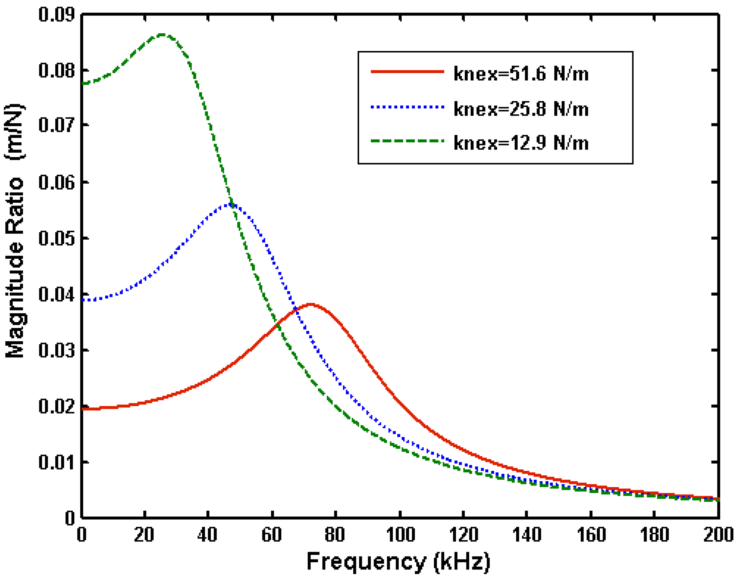
We looked at several different hole sizes and ambient pressures. Figure 3 shows the frequency response for different leg stiffness at atmospheric pressure (101,000 Pa) and with a hole size of 67 μm × 67 μm. When the stiffness increases, both the resonant frequency and Q value increase. When the stiffness is 12.9 N/m, the peak in the resonant frequency is almost flat. For lower stiffness, the structure would be over damped at atmospheric pressure. When the stiffness increases to 51.6 N/m, the resonant peak is sharper, and a shift in resonant peak would be fairly easy to detect. This figure shows that stiffness plays an important role in the performance of a resonant mass sensor.

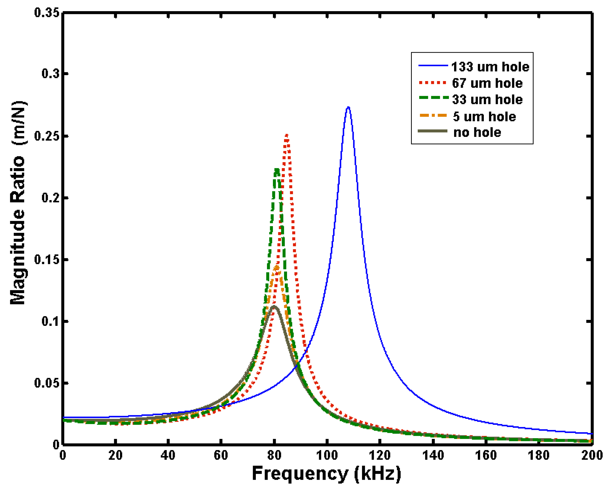
Figure 4 compares the frequency responses for different hole sizes. The leg stiffness is 51.6 N/m, and the pressure of the surrounding environment is 3,000 Pa. This figure shows the effect of a low ambient pressure: even with low leg stiffness, the Q values are better than in Figure 3.

Figure 3. Effect of leg stiffness on frequency response of square plate resonator with 67 μm × 67 μm hole at atmospheric pressure.

Figure 3. Effect of leg stiffness on frequency response of square plate resonator with 67 μm × 67 μm hole at atmospheric pressure.

Figure 4. Effect of hole size on frequency response of square plate resonator with leg stiffness of 51.6 N/m and 3,000 Pa ambient pressure.

Figure 4. Effect of hole size on frequency response of square plate resonator with leg stiffness of 51.6 N/m and 3,000 Pa ambient pressure.

3. Comparison with FEM Model

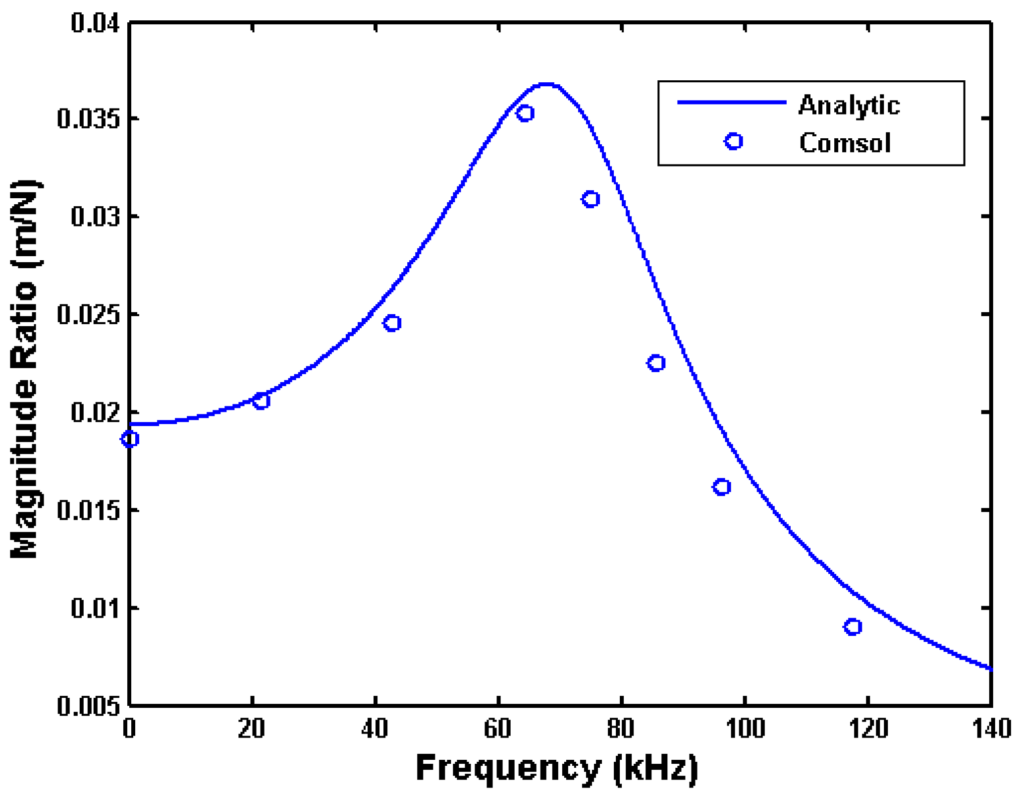
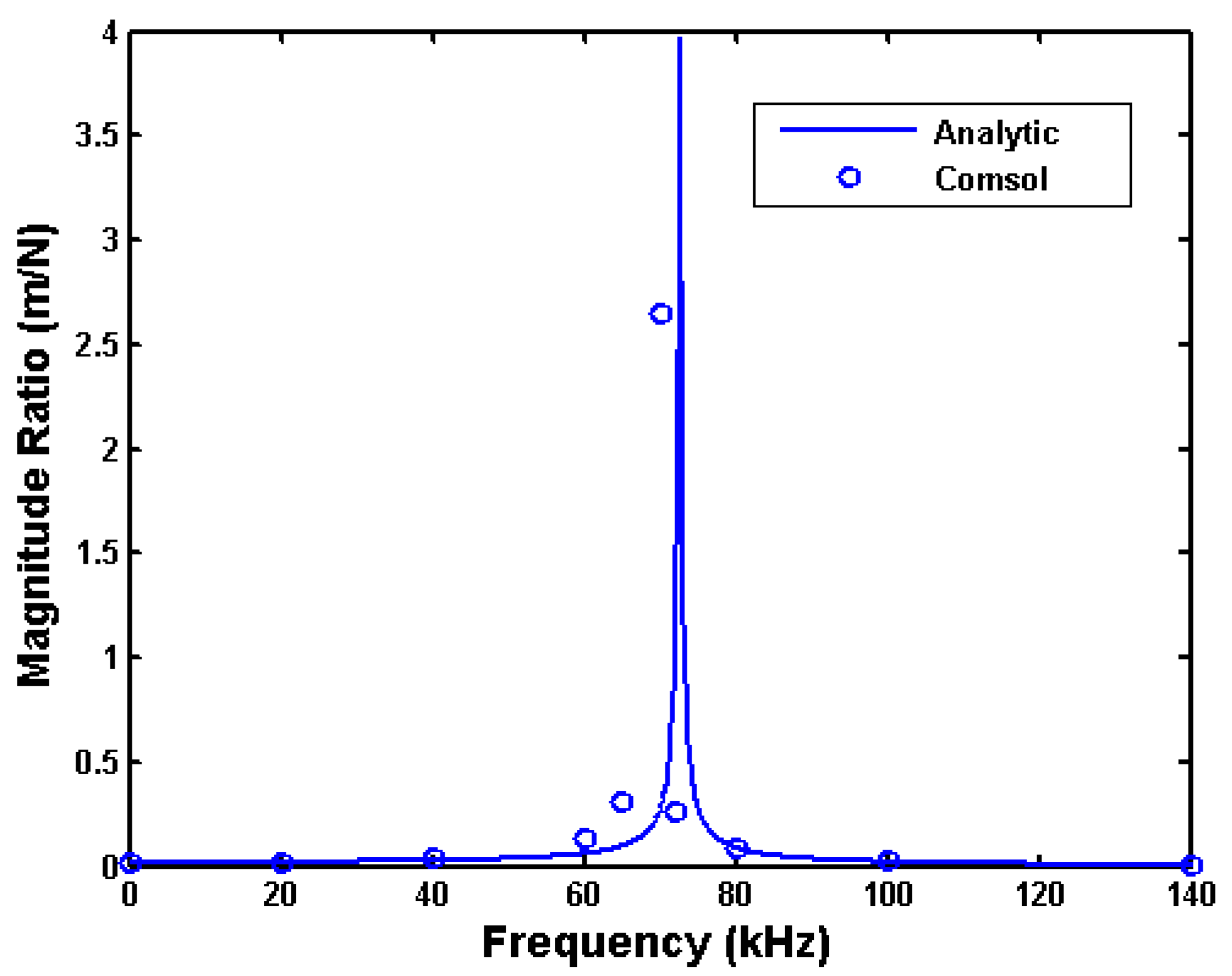
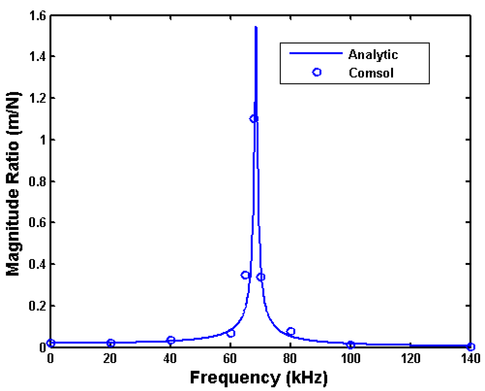
We validated the analytical model using numerical finite element Comsol simulations. Figure 5, Figure 6, Figure 7 and Figure 8 show the frequency responses for four sets of conditions. The conditions span different hole sizes, air pressures, and leg stiffnesses that produce a wide range of resonant frequency and damping characteristics. The figures show that the analytical model predicts the frequency responses fairly well for this wide range of hole sizes and air pressures.

Figure 5. Comparison of analytical and numerical frequency responses for square plate with 67 μm × 67 μm hole, at atmospheric pressure, with folded leg stiffness of 51.65 N/m.

Figure 5. Comparison of analytical and numerical frequency responses for square plate with 67 μm × 67 μm hole, at atmospheric pressure, with folded leg stiffness of 51.65 N/m.

Figure 6. Comparison of analytical and numerical frequency responses for square plate with 67 μm × 67 μm hole, at ambient pressure of 300 Pa, with folded leg stiffness of 51.65 N/m.

Figure 6. Comparison of analytical and numerical frequency responses for square plate with 67 μm × 67 μm hole, at ambient pressure of 300 Pa, with folded leg stiffness of 51.65 N/m.

Figure 7. Comparison of analytical and numerical frequency responses for square plate with 5 μm × 5 μm hole, at ambient pressure of 300 Pa, with folded leg stiffness of 51.65 N/m.

Figure 7. Comparison of analytical and numerical frequency responses for square plate with 5 μm × 5 μm hole, at ambient pressure of 300 Pa, with folded leg stiffness of 51.65 N/m.

Figure 8. Comparison of analytical and numerical frequency responses for square plate with no hole, at ambient pressure of 300 Pa, with folded leg stiffness of 0.5165 N/m.

Figure 8. Comparison of analytical and numerical frequency responses for square plate with no hole, at ambient pressure of 300 Pa, with folded leg stiffness of 0.5165 N/m.

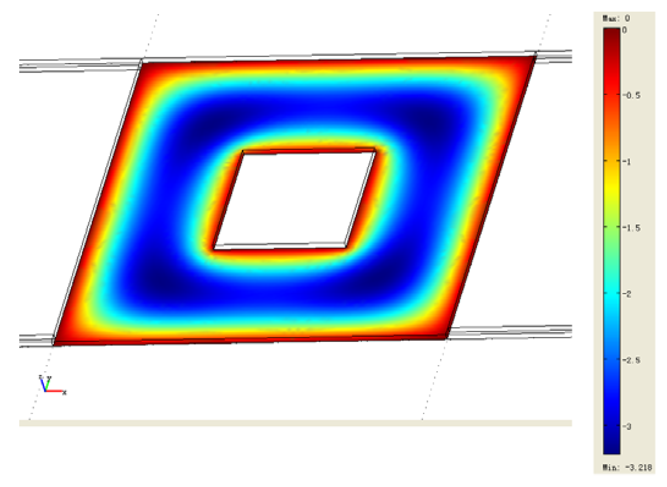
Figure 9 shows the finite element simulation of the pressure distribution underneath the closed and perforated plate in the equilibrium position during vibration. The ambient pressure is 300 Pa and the amplitude of vibration is 0.2 μm in the 4 μm gap at 67 KHz. The pressure around the edge of the plate and the hole is close to zero. The largest pressure is 3.2 Pa which appears in the corner regions.

Figure 9. Distribution of pressure by damping.

Figure 9. Distribution of pressure by damping.

4. Design Optimization Objective Function

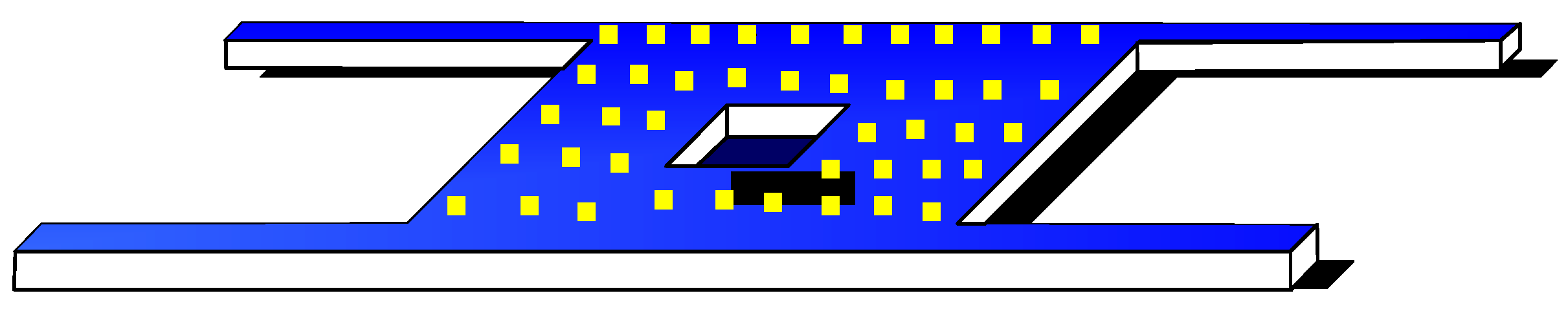
In a sensor application, the flat plate is covered by a polymer sensing layer as shown in Figure 10. The small golden balls represent chemical vapor molecules that have bound to the polymer and added mass to the plate. Our goal was to find the optimum hole size that would balance the need for large plate area for sensing and electrostatic actuation against large hole area for low air damping and high resonator Q.

Figure 10. Flat plate sensor structure.

Figure 10. Flat plate sensor structure.

As a case study, we considered the absorption of a nerve gas analog (DMMP) onto a PPESO₃Na⁺ polymer coating [15]. We estimated that a 100 nm thick polymer layer could absorb between 3.1 mg/m² and 8.1 mg/m². To be conservative, we considered the addition of 0.056 mg/m² of DMMP to the entire plate area. For a 200 μm × 200 μm plate with 67 μm × 67 μm hole, the total added mass would be 2 × 10⁻¹⁰ g. We then calculated the effect of the absorbed mass on the resonant peak of the sensor structure for three different ambient pressure conditions. Table 2 shows the change in frequency and amplitude of the resonant peak. Large changes in both characteristics are desirable for a sensitive sensor.

Table 2. Effect of the addition of nerve gas analog on resonant frequency and peak height when 2 × 10⁻¹² g mass is added to a 200 μm × 200 μm × 3 μm silicon plate with 67 μm × 67 μm hole, with leg stiffness of 5.16 N/m, and 3 μm gap between plate and substrate.

	Nominal Resonant Frequency	Change in Resonant Frequency	Nominal Peak Magnitude Ratio	Change in Peak Magnitude Ratio
3 Pa	22.88 kHz	−14 Hz	287.5 m/N	−26.3 m/N
300 Pa	25.92	−16	1.622	−0.005
3,000 Pa	39.92	−33	0.07753	−0.00014

Table 2. Effect of the addition of nerve gas analog on resonant frequency and peak height when 2 × 10⁻¹² g mass is added to a 200 μm × 200 μm × 3 μm silicon plate with 67 μm × 67 μm hole, with leg stiffness of 5.16 N/m, and 3 μm gap between plate and substrate.

	Nominal Resonant Frequency	Change in Resonant Frequency	Nominal Peak Magnitude Ratio	Change in Peak Magnitude Ratio
3 Pa	22.88 kHz	−14 Hz	287.5 m/N	−26.3 m/N
300 Pa	25.92	−16	1.622	−0.005
3,000 Pa	39.92	−33	0.07753	−0.00014

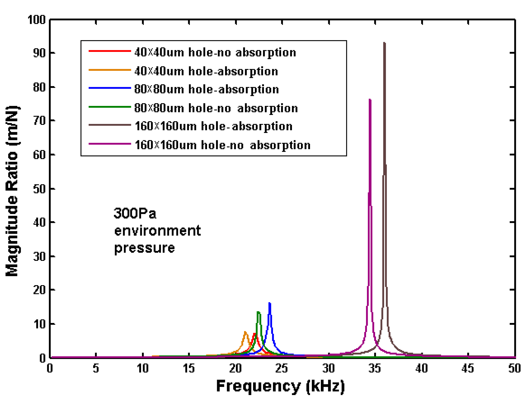
In addition to ambient pressure, the effect of hole size was investigated. For these trials, we determined the frequency responses before and after adding 10% to the mass of the plate. The 10% mass change means the absolute changes in mass are different for each plate because the plate areas differ. Figure 11 compares the change in frequency response for three hole sizes in a 200 μm × 200 μm plate. In all three cases, the peak amplitude drops and shifts to a slightly lower frequency when mass is added. The resonant frequency for the 160 μm × 160 μm hole plate is much higher than the others because the large hole has eliminated most of the plate’s mass.

Figure 11. Effect of a 10% mass increase on the frequency response of three plates.

Figure 11. Effect of a 10% mass increase on the frequency response of three plates.

The design optimization process requires a meaningful measure of the change in frequency response. One measure is RMS, defined as:

$$RMS=\sqrt{\frac{{\displaystyle \sum _{i=1}^n{\left(a_{1i}-a_{2i}\right)}^2}}{n}}$$

(10)

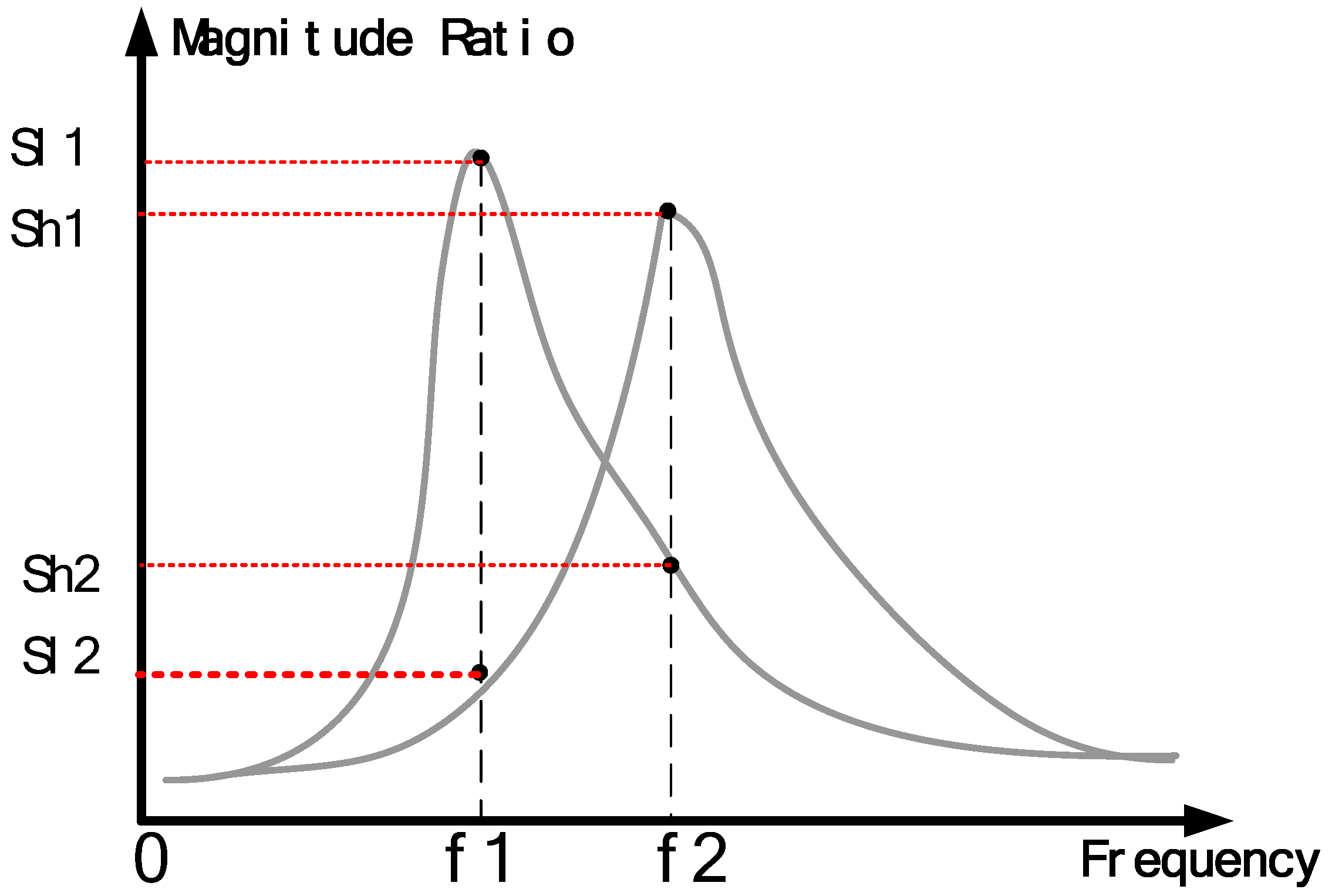
Here a_1i means the amplitude under the i_th frequency step in the frequency response curve with no absorption and a_2i means the amplitude under the i_th frequency step in the frequency response curve with absorption. One difficulty with RMS is that it depends on the frequency range over which it is calculated. To simplify the calculation and remove the need to choose a frequency range, we propose a new measure Q_s:

$$Q_s=\sqrt{\frac{{\left(S_{l1}-S_{l2}\right)}^2+{\left(S_{h1}-S_{h2}\right)}^2}{2}}$$

(11)

where S_l1, S_l2, S_h1, and S_h2 are as defined in Figure 12. Q_s is essentially a two point RMS, making use of the two resonant frequencies with and without absorption.

Figure 12. Illustration of the definition of Q_s.

Figure 12. Illustration of the definition of Q_s.

We compared the values of RMS and Q_s for hypothetical systems having a transfer function of the form:

$$\frac{dx}{dF}=\frac{1}{m{s}^2+bs+k}$$

(12)

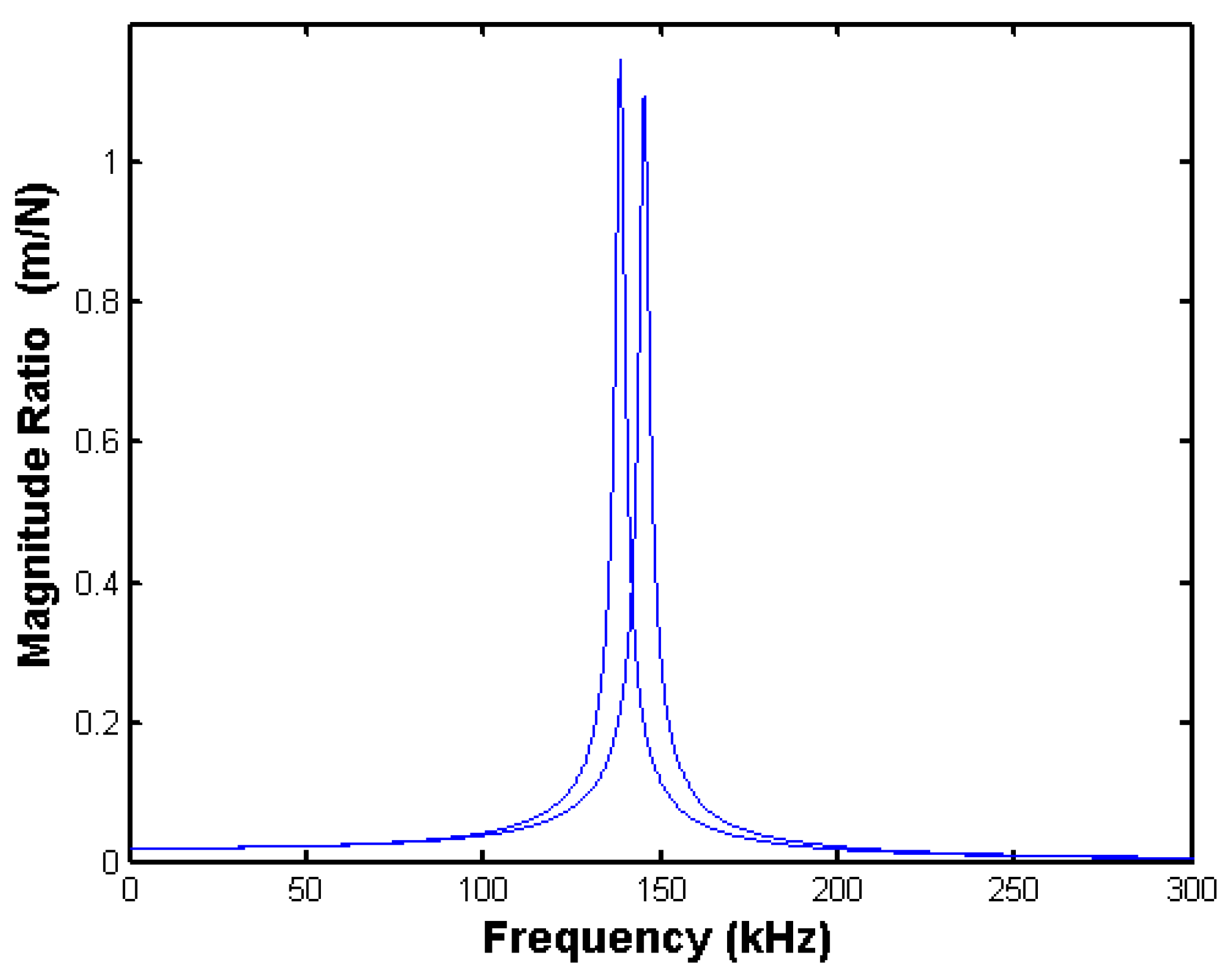
The original mass is m_o, and the mass after chemical absorption is m_o + Δm. As an example, Figure 13 compares the frequency responses for a system before and after a 10% change in mass. The system parameters are: m_o = 6 × 10⁻¹¹ kg, Δm = 0.1m_o, b = 1 × 10⁻⁶ N-s/m, and k = 50 N/m. The resonant peak drops from 145.3 kHz to 138.5 kHz with the extra mass.

Figure 13. Effect of 10% mass change on frequency response.

Figure 13. Effect of 10% mass change on frequency response.

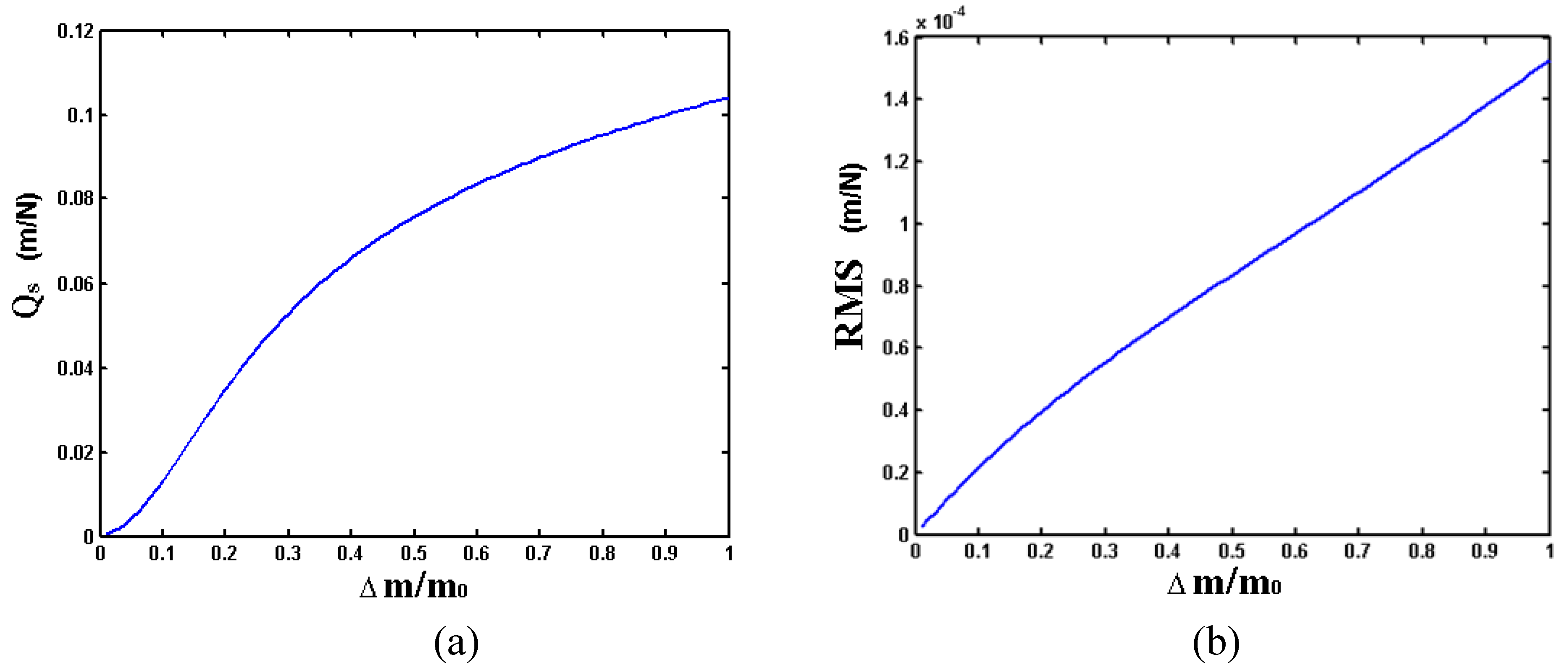
Figure 14 compares the RMS and Q_s values as a function of the percent mass change. The RMS was calculated using a frequency range of 0 Hz to 400 kHz with a frequency step of 100 Hz.

Figure 14. Comparison of Q_s and RMS as a function of mass change.

Figure 14. Comparison of Q_s and RMS as a function of mass change.

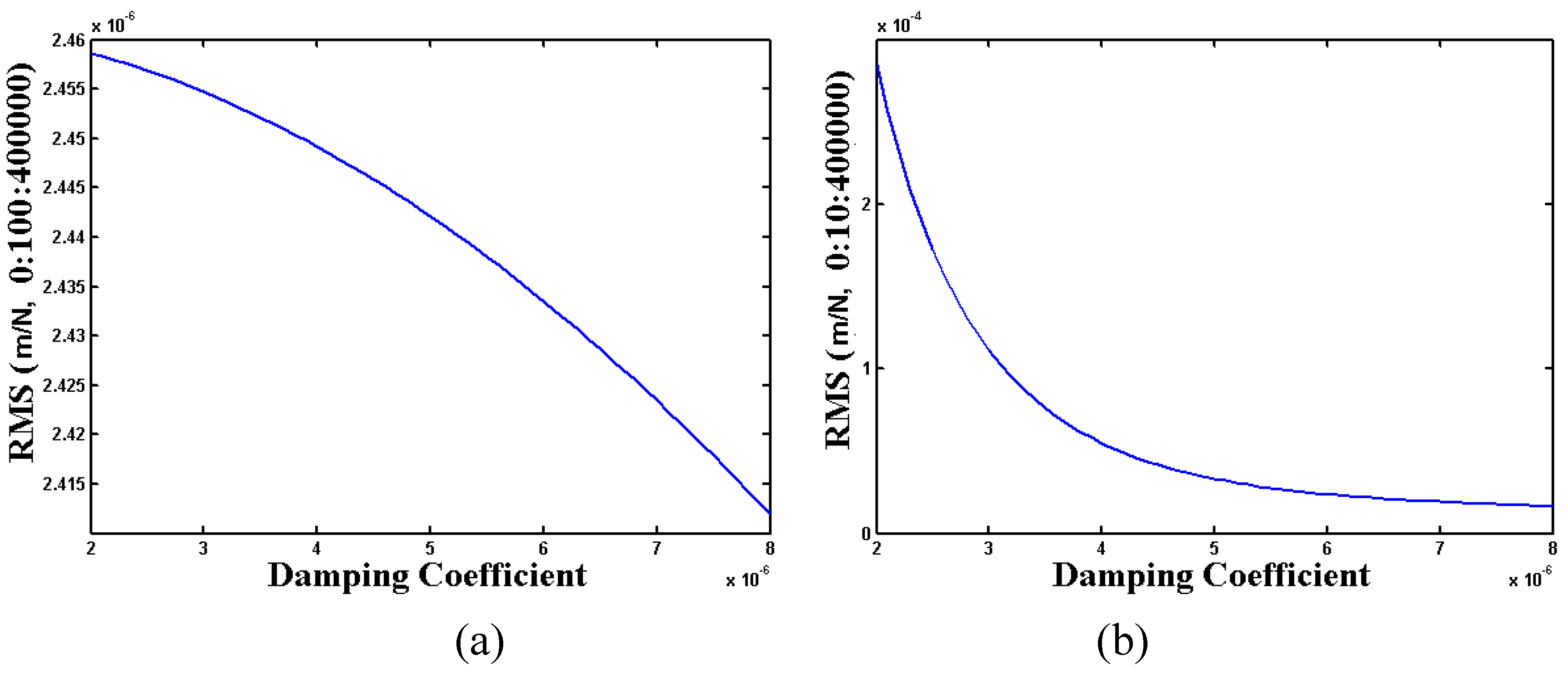
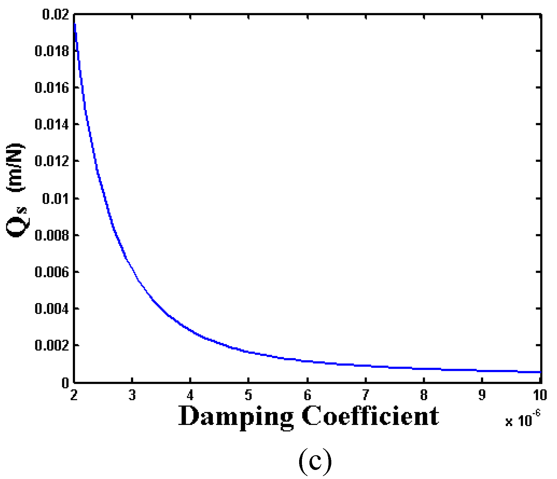
When the mass increases from zero to twice its original value, both the Q_s and the RMS increase monotonically, with RMS increasing more linearly than Q_s. Next, we looked at how Q_s and RMS change with damping coefficient. In Figure 15, the RMS results are calculated using a 0 to 400 kHz frequency range and with a 100 Hz frequency step in (a) and a 10 Hz frequency step in (b). The smaller frequency step produces a result that looks similar to the Q_s result. All three measures decrease as damping increases, reinforcing the importance of a sensor with high Q (or low damping).

Figure 15. Comparison of RMS and Q_s for different damping coefficients.

Figure 15. Comparison of RMS and Q_s for different damping coefficients.

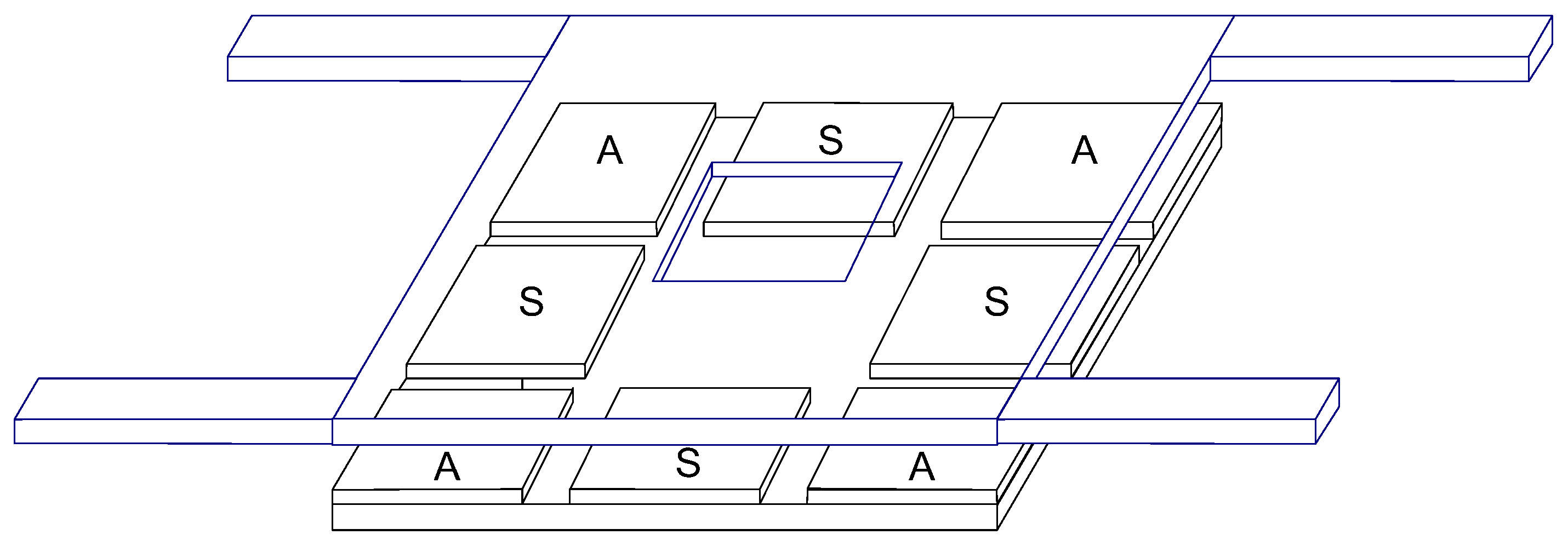
The parameter Q_s will now be used to determine an optimum hole size for a flat plate resonator. Consider the system shown in Figure 16. It is a flat plate connected to the substrate with four springs at its corners. The sensing electrode is shown as one of the two black electrodes underneath the suspension plate, and the actuation electrode is shown as another electrode. There is a hole in the middle of suspension plate. In our optimization problem we will use half of the plate’s area as the sensing electrode, and half as the actuation electrode.

Figure 16. Schematic of square plate oscillator showing actuation and sensing electrodes.

Figure 16. Schematic of square plate oscillator showing actuation and sensing electrodes.

In the frequency responses discussed thus far, the magnitude ratio is calculated by dividing a displacement output by a force input x/F. However, the input to the actual device is a voltage, and the output of the actual device is capacitance. The magnitude ratio is thus ΔC/ΔV. We further simplify the optimization problem by considering small vibrations about an offset displacement. In this way we linearize the voltage-to-electrostatic force and capacitance-to-displacement relationships. For this problem, the magnitude ratio of interest is ΔC/ΔV. This new magnitude ratio can be found from:

$$\frac{dC}{dV}=\frac{dx}{dF}\frac{dC}{dx}\frac{dF}{dV}$$

(13)

For the rigid plate attached to the substrate with folded leg springs:

$$\frac{dx}{dF}=\frac{1}{m{s}^2+bs+k}$$

(14)

where b and k incorporate the effects of squeeze film damping (Equations 1-6). The system will be oscillated with small amplitudes around a setpoint with displacement x₀ (measured as capacitance C₀) at a force F₀ (realized by applying the voltage V₀). The equation for capacitance is:

$$C=\frac{\epsilon A_s}{g_o-x}$$

(15)

Differentiating the C equation:

$$\frac{dC}{dx}=\frac{\epsilon A_s}{{\left(g_o-x_o\right)}^2}$$

(16)

The actuation force is:

$$F=\frac{\epsilon A_a{V}^2}{2{\left(g_o-x_o\right)}^2}=kx$$

(17)

where A_a is the actuating area, V is the applied voltage, and k is the stiffness of the corner springs. The displacement x, depends on V but also on k. To obtain an expression for dF/dV that doesn’t have x in it, we substitute x = F/k in Equation (17). After rearranging, we obtain:

$$\frac{1}{k^2}{F}^3-\frac{2g_o}{k}{F}^2+g_o^{2}F-\frac{\epsilon A_a{V}^2}{2}=0$$

(18)

Differentiating this equation gives:

$$\frac{3F^2}{k^2}dF-\frac{4g_{o}F}{k}dF+g_o^{2}dF-\epsilon A_{a}VdV=0$$

(19)

Solving for dF/dV yields:

$$\frac{dF}{dV}=\frac{\epsilon A_a{V}_o}{\left(3\frac{F^2}{k^2}-4g_o\frac{F}{k}+g_o^2\right)}$$

(20)

The displacement x can be substituted for F/k. At the setpoint of V_o and F_o, the slope is:

$$\frac{dF}{dV}=\frac{\epsilon A_a{V}_o}{\left(g_o-x_o\right)\left(g_o-3x_o\right)}$$

(21)

Combining the factors in Equations (14), (16), and (21) yields:

$$\frac{dC}{dV}=\frac{{\epsilon }^2{A}_s{A}_a{V}_o}{{\left(g_o-x_o\right)}^3\left(g_o-3x_o\right)}\frac{1}{m{s}^2+bs+k}$$

(22)

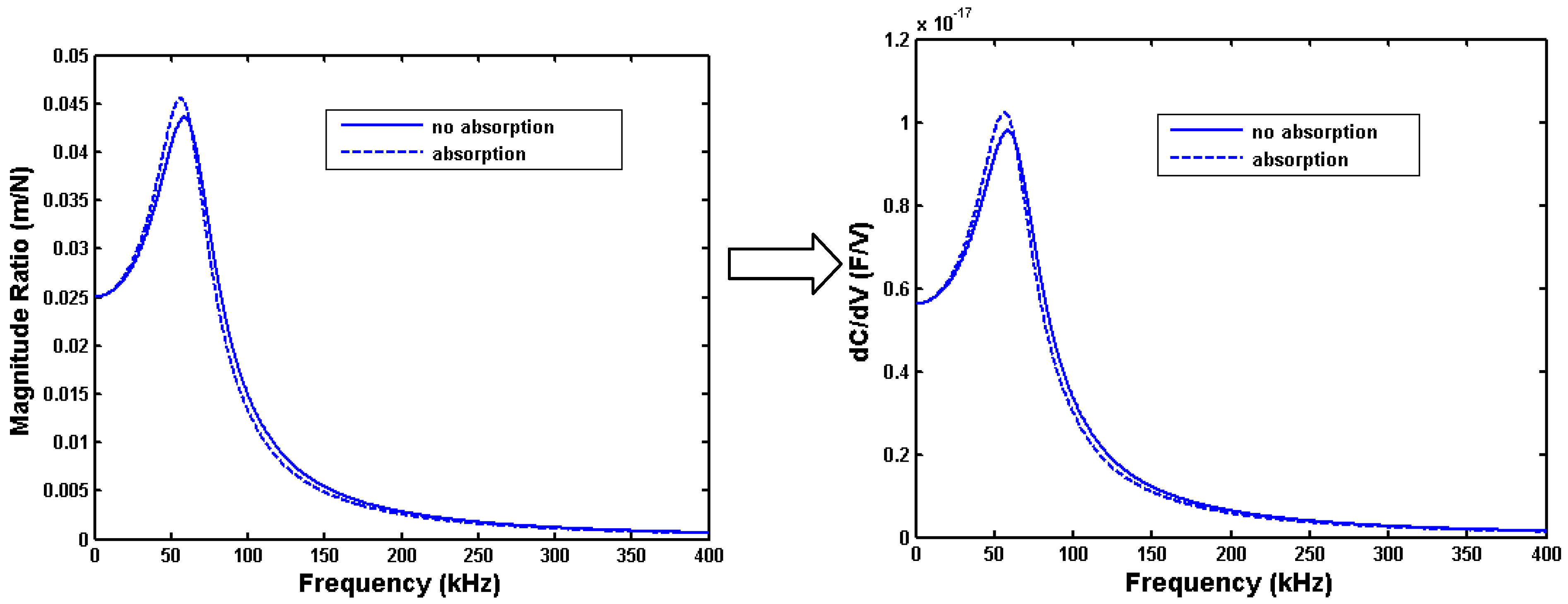
Figure 17 shows the frequency responses of a system using two different types of magnitude ratios. The system consists of a 200 μm × 200 μm × 3 μm plate with 4 μm gap and supported by four folded beams with the stiffness of 51.65 N/m. The hole is centered in the middle of the plate. Half of the plate area is used for actuation and the other half for capacitive sensing. The surrounding air pressure is 101,000 Pa, and the mass change due to absorbed vapor will be 10%. The setpoint voltage V_o is 10 V. The magnitude ratio in the first plot is in the form of displacement over force, and the ratio in the second plot is capacitance change over input voltage change. Note that the second plot of dC/dV differs from the first one of dx/dF only by a constant. As shown in Equation (22), that constant depends on the areas available for sensing and actuation.

Figure 17. Effect of hole size on sensor sensitivity (defined as Q_s) for 200 μm × 200 μm × 3 μm plate, with g_o = 4 μm, V_o = 10 V, P_a = 101,000 Pa, k_flex = 51.65 N/m, Δm/m_o = 0.1.

Figure 17. Effect of hole size on sensor sensitivity (defined as Q_s) for 200 μm × 200 μm × 3 μm plate, with g_o = 4 μm, V_o = 10 V, P_a = 101,000 Pa, k_flex = 51.65 N/m, Δm/m_o = 0.1.

5. Determining Optimal Hole Size

The pieces are now in place to look at an optimal design. The goal is to maximize Q_s as calculated from frequency responses that use dC/dV as the magnitude ratio. The square plate is assumed to be 200 μm × 200 μm × 3 μm with 4 μm gap. The stiffness of structure is 51.65 N/m and the setpoint voltage V_o is 10 V. The surrounding air pressure is 101,000 Pa, and the mass change due to absorbed vapor will be 10%. We wish to find the hole size that maximizes sensor sensitivity. 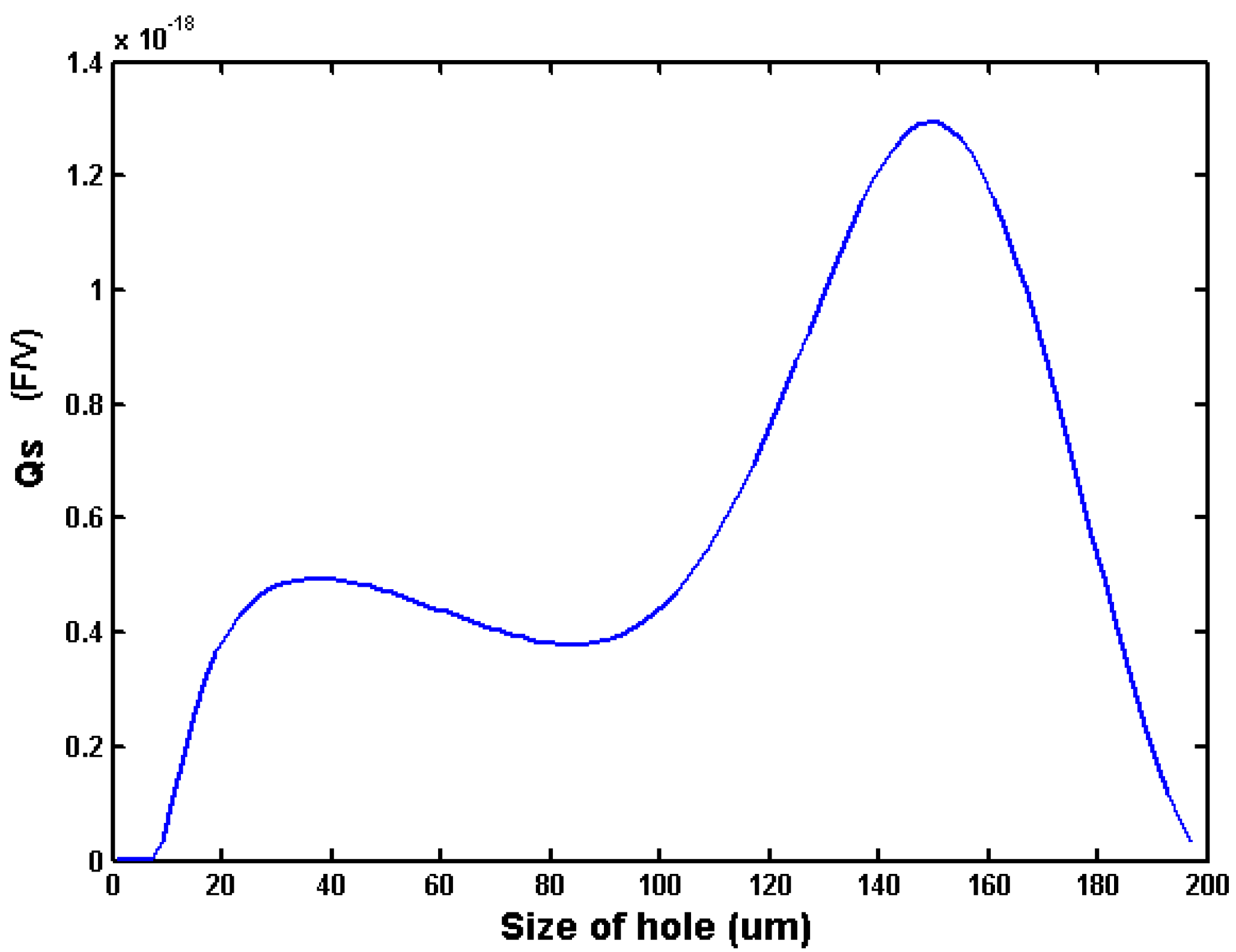Figure 18 shows how Q_s changes with hole size. The units for Q_s are farads/volt. Note that the highest Q_s occurs for a hole size of about 149 μm. In other words, this is the hole size that will yield the best sensitivity for this particular plate size, gap, setpoint voltage, and ambient air pressure.

Figure 18. Effect of hole size on sensor sensitivity (defined as Q_s) for 200 μm × 200 μm × 3 μm plate, with g_o = 4 μm, V_o = 10 V, P_a = 101,000 Pa, k_flex = 51.65 N/m, Δm/m_o = 0.1.

Figure 18. Effect of hole size on sensor sensitivity (defined as Q_s) for 200 μm × 200 μm × 3 μm plate, with g_o = 4 μm, V_o = 10 V, P_a = 101,000 Pa, k_flex = 51.65 N/m, Δm/m_o = 0.1.

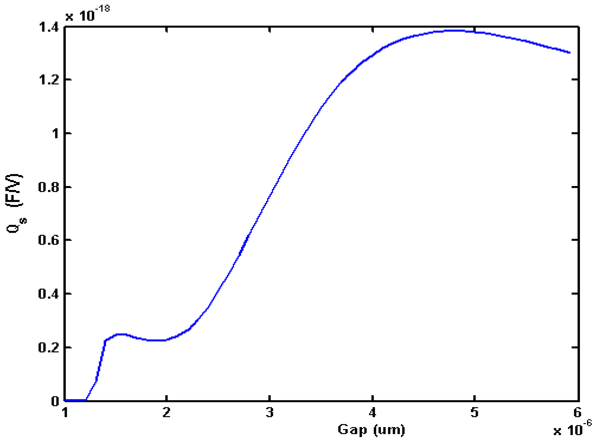
Given a particular hole size, there is also an optimum gap. Figure 19 shows how Q_s changes with gap when the hole size is fixed at 149 μm × 149 μm. A large gap will have a favorable effect on a resonator’s Q. However, the amplitude of motion will fall off as the gap increases, thus explaining why Q_s decreases for a gap above about 4.8 μm in Figure 19.

Figure 19. Effect of gap on sensor sensitivity for 200 μm × 200 μm × 3 μm plate, with V_o = 10 V, P_a = 101,000 Pa, k_flex = 51.65 N/m, Δm/m_o = 0.1, hole size of 149 μm × 149 μm.

Figure 19. Effect of gap on sensor sensitivity for 200 μm × 200 μm × 3 μm plate, with V_o = 10 V, P_a = 101,000 Pa, k_flex = 51.65 N/m, Δm/m_o = 0.1, hole size of 149 μm × 149 μm.

In the examples above, the electrode area was split evenly between actuation area and capacitive sensing area. We checked to see if there was a more favorable split. We calculated Q_s while varying the ratio of actuation area to the total plate area from 5% to 95%. Figure 20 shows that the maximum value occurs at 50% (where the areas are evenly split). After looking at Equation (22), this result makes sense. The amplitude in the frequency response depends on the product of A_a and A_s. Given that the sum of A_a and A_s is fixed, the maximum product occurs when A_a and A_s are equal.

Figure 20. Effect of the actuation area on sensitivity for 200 μm × 200 μm × 3 μm plate, with V_o = 10 V, g_o = 4 μm, P_a = 101,000 Pa, k_flex = 51.65 N/m, Δm/m_o = 0.1, hole size of 149 μm × 149 μm.

Figure 20. Effect of the actuation area on sensitivity for 200 μm × 200 μm × 3 μm plate, with V_o = 10 V, g_o = 4 μm, P_a = 101,000 Pa, k_flex = 51.65 N/m, Δm/m_o = 0.1, hole size of 149 μm × 149 μm.

Finally, we looked at finding the optimum combination of hole size and gap. Figure 21 plots Q_s versus both hole size and gap for the 200 μm × 200 μm × 3 μm plate. The peak value of Q_s (1.81x10^-18 farads/volt) occurs when the gap is 5.2 μm and the hole size is 144 μm × 144 μm.

Figure 21. Effect of the hole size and gap on sensitivity for 200 μm × 200 μm × 3 μm plate, with V_o = 10 V, P_a = 101,000 Pa, k_flex = 51.65 N/m, Δm/m_o = 0.1.

Figure 21. Effect of the hole size and gap on sensitivity for 200 μm × 200 μm × 3 μm plate, with V_o = 10 V, P_a = 101,000 Pa, k_flex = 51.65 N/m, Δm/m_o = 0.1.

6. Conclusions

In summary, we have adopted an analytical squeeze film damping model that adequately replicates finite element modeling results over a wide range of conditions. In addition, we have defined an objective function that permits the calculation of an optimal design (given particular constraints) that takes into account electrostatic actuation, capacitive sensing, and squeeze film damping. Results for optimum hole size, gap, and electrode area partitioning have been presented. Future work involves investigating additional factors (such as setpoint voltage, ambient pressure, and expected mass change) as well as additional geometries (such as non-square plates, multiple holes, and bending cantilevers).