Temporal Prediction of Paralytic Shellfish Toxins in the Mussel Mytilus galloprovincialis Using a LSTM Neural Network Model from Environmental Data


Abstract
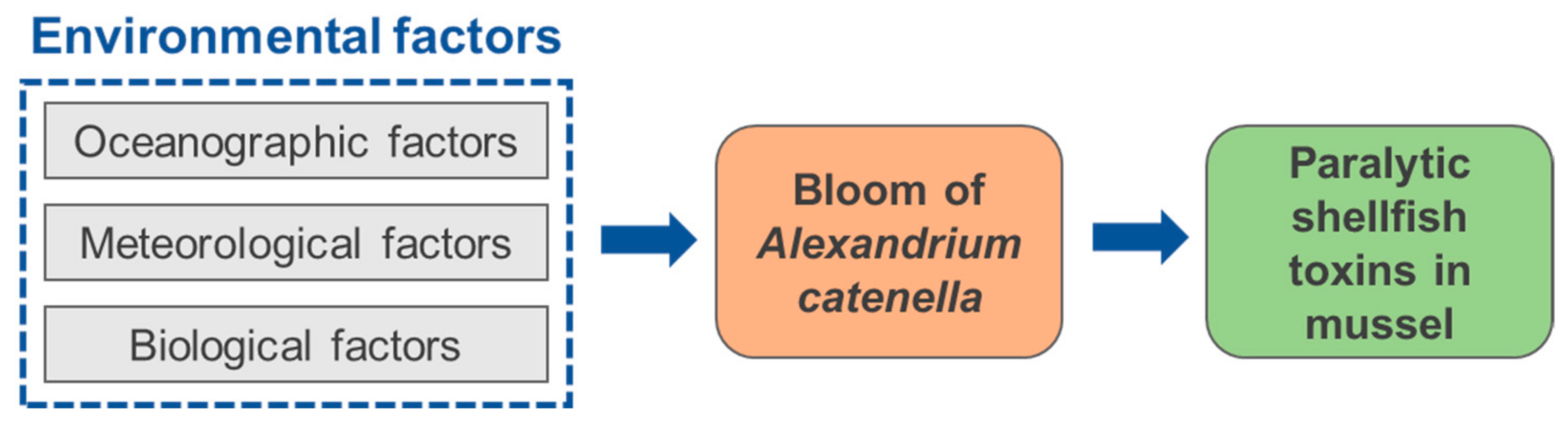
1. Introduction
2. Results
2.1. Periodic Tendency of Paralytic Shellfish Toxins Outbreak
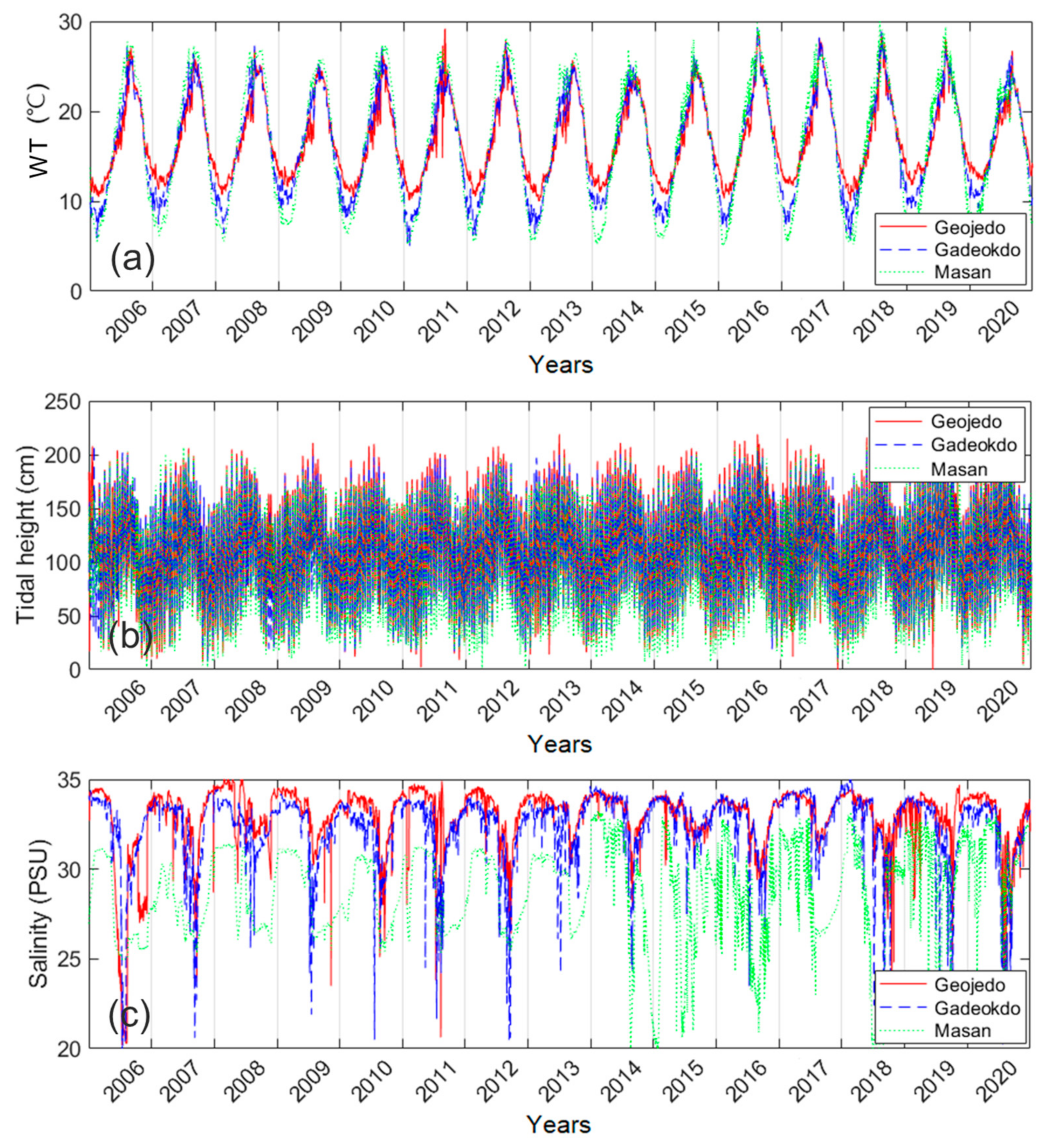
2.2. Gap-Filling of Environmental Factors
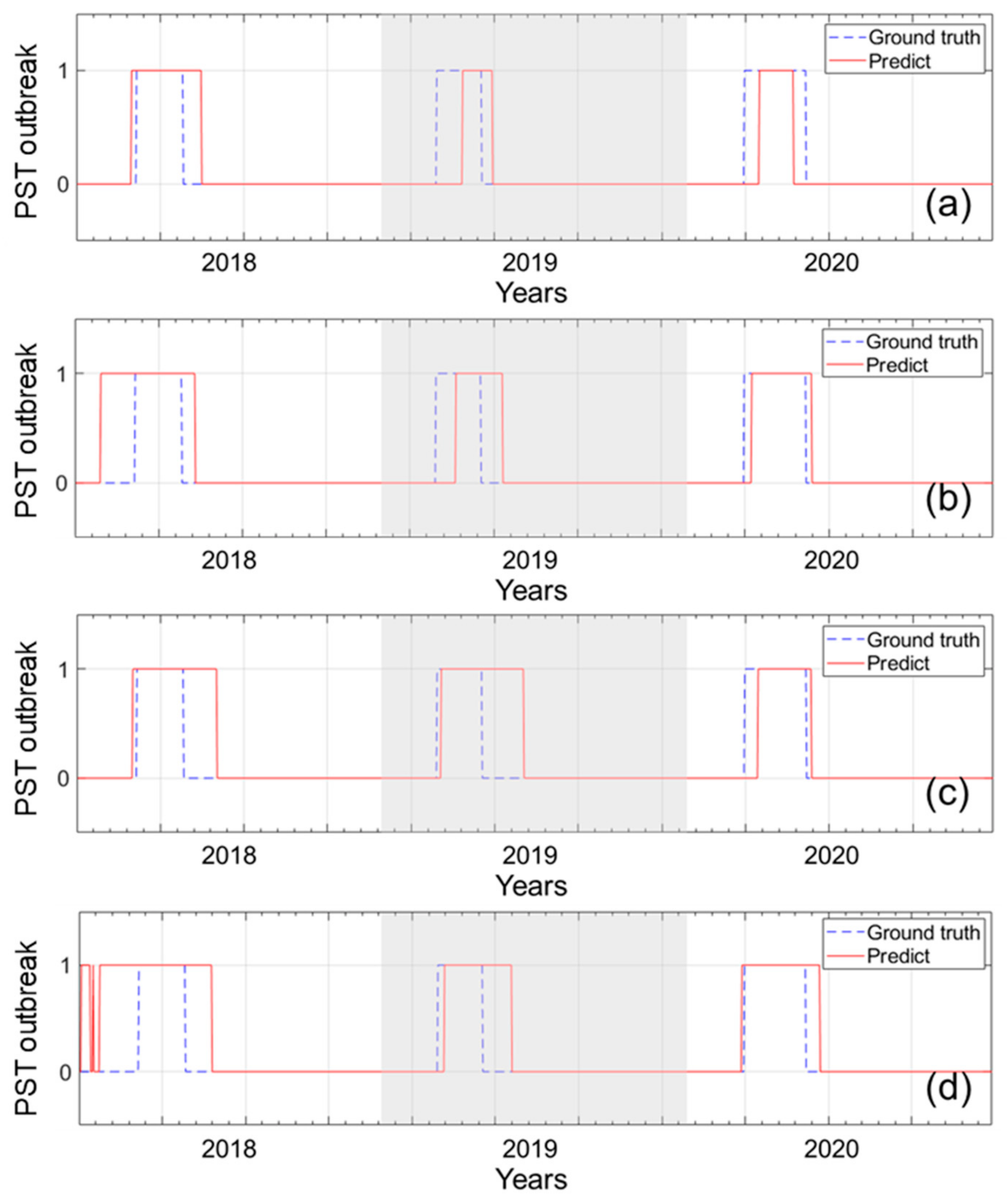
2.3. Temporal Prediction of PSTs Outbreak
3. Discussion
3.1. Performance of LSTM Models
3.2. Environmental Factors
4. Conclusions
5. Materials and Methods
5.1. Study Area
5.2. Data
5.3. LSTM Neural Network Model
5.4. Performance Assessment
Author Contributions
Funding
Institutional Review Board Statement
Informed Consent Statement
Data Availability Statement
Conflicts of Interest
References
- Wang, J.; Wu, J. Occurrence and potential risks of harmful algal blooms in the East China Sea. Sci. Total Environ. 2009, 407, 4012–4021. [Google Scholar] [CrossRef] [PubMed]
- Ishikawa, A.; Hattori, M.; Ishi, K.I.; Kulis, D.M.; Anderson, D.M.; Imai, I. In situ dynamics of cyst and vegetative cell populations of the toxic dinoflagellate Alexandrium catenella in Ago Bay, central Japan. J. Plankton Res. 2014, 36, 1333–1343. [Google Scholar] [CrossRef] [PubMed]
- Taylor, F.J.R.; Fukuyo, Y.; Larsen, J. Taxonomy of harmful dinoflagellates. In Manual on Harmful Marine Microalgae; IOC Manuals and Guides No. 33. IOC of UNESCO; Hallegraeff, G.M., Abderson, D.M., Cembella, A.D., Eds.; United Nations Educational, Scientific and Cultural Organization (UNESCO): Paris, France, 2003; pp. 281–317. [Google Scholar]
- Hallegrae, G.M. A review of harmful algal blooms and their apparent global increase. Phycologia 1993, 32, 79–99. [Google Scholar] [CrossRef]
- Anderson, D.M. Turning back the harmful red tide. Nature 1997, 388, 513–514. [Google Scholar] [CrossRef]
- Shumway, S.E. A review of the effects of algal blooms on shellfish and aquaculture. J. World Aquac. Soc. 1990, 21, 65–104. [Google Scholar] [CrossRef]
- Smayda, T.J. Harmful algal blooms: Their ecophysiology and general relevance to phytoplankton blooms in the sea. Limnol. Oceanogr. 1997, 42, 1137–1153. [Google Scholar] [CrossRef]
- Chang, D.S.; Shin, I.S.; Pyeun, J.H.; Park, Y.H. A study on paralytic shellfish poison of sea messel Mytilus edulis. Bull. Korean Soc. Fish. Technol. 1987, 20, 293–299. [Google Scholar]
- Lee, J.S.; Shin, I.S.; Kim, Y.M.; Chang, D.S. Parlytic shellfish toxins in the mussel, Mytilus edulis, caused the shellfish poisoning accident at Geoje, Korea, in 1996. J. Korean Fish. Soc. 1997, 30, 158–160. [Google Scholar]
- Han, M.S.; Jeon, J.K.; Kim, Y.O. Occurrence of dinoflagellate Alexandrium tamarense, a causative organism of paralytic shellfish posisoning in Chinhae Bay, Korea. J. Plankton. Res. 1992, 14, 1581–1592. [Google Scholar] [CrossRef]
- Forecast·Breaking News of the National Institute of Fisheries Science (NIFS). Available online: https://www.nifs.go.kr/bbs?id=shellfish (accessed on 6 January 2022).
- Anderson, D.M.; Alpermann, T.J.; Cembella, A.D.; Collos, Y.; Masseret, E.; Montreosr, M. The globally distributed genus Alexandrium: Multifaceted roles in marine ecosystems and impacts on human health. Harmful Algae 2012, 14, 10–35. [Google Scholar] [CrossRef]
- Baek, S.H.; Choi, J.M.; Lee, M.; Park, B.S.; Zhang, Y.; Arakawa, O.; Takatani, T.; Jeon, J.K.; Kim, Y.O. Change in Paralytic Shellfish Toxins in the Mussel Mytilus galloprovincialis Depending on Dynamics of Harmful Alexandrium catenella (Group I) in the Geoje Coast (South Korea) during Bloom Season. Toxins 2020, 12, 442. [Google Scholar] [CrossRef]
- Ichimi, K.; Suzuki, T.; Yamasaki, M. Non-selective retention of PSP toxins by the mussel Mytilus galloprovincialis fed with the toxic dinoflagellate Alexandrium tamarense. Toxicon 2001, 39, 1917–1921. [Google Scholar] [CrossRef]
- Kim, Y.O.; Park, M.H.; Han, M.S. Role of cyst germination in the bloom initiation of Alexandrium tamarense (Dinophyceae) in Masan Bay, Korea. Aquat. Microb. Ecol. 2002, 29, 279–286. [Google Scholar] [CrossRef]
- Lee, H.O.; Choi, K.H.; Han, M.S. Spring bloom of Alexandrium tamarense in Chinhae Bay, Korea. Aquat. Microb. Ecol. 2003, 33, 271–278. [Google Scholar] [CrossRef][Green Version]
- Shin, J.; Kim, S.M.; Son, Y.B.; Kim, K.; Ryu, J.H. Early Prediction of Margalefidinium polykrikoides Blooms Using a LSTM Neural Network Model in the South Sea of Korea. J. Coast. Res. 2019, 90, 236–242. [Google Scholar] [CrossRef]
- Liu, Y.; Liu, P.; Wang, X.; Zhang, X.; Qin, Z. A study on water quality prediction by a hybrid dual channel CNN-LSTM model with attention mechanism. In Proceedings of the International Conference on Smart Transportation and City Engineering 2021, Chongqing, China, 10 November 2021; Volume 12050, pp. 797–804. [Google Scholar]
- Box, G.E.; Jenkins, G.M.; Reinsel, G.C.; Ljung, G.M. Time Series Analysis: Forecasting and Control; John Wiley & Sons, Inc.: New York, NY, USA, 2015. [Google Scholar]
- Lee, Y.S.; Tong, L.I. Forecasting time series using a methodology based on autoregressive integrated moving average and genetic programming. Knowl. Based Syst. 2011, 24, 66–72. [Google Scholar] [CrossRef]
- Lam, C.Y.; Ip, W.H.; Lau, C.W. A business process activity model and performance measurement using a time series ARIMA intervention analysis. Expert Syst. Appl. 2009, 36, 6986–6994. [Google Scholar] [CrossRef]
- Lippi, M.; Bertini, M.; Frasconi, P. Short-term traffic flow forecasting: An experimental comparison of time-series analysis and supervised learning. IEEE Trans. Intel. Transport. Syst. 2013, 14, 871–882. [Google Scholar] [CrossRef]
- Kim, G.B.; Choi, M.R.; Hwang, C.I. Comparison of missing value imputations for groundwater levels using multivariate ARIMA, MLP, and LSTM. J. Geo. Soci. Korea 2020, 56, 561–569. [Google Scholar] [CrossRef]
- Zhu, B.; Wei, Y. Carbon price forecasting with a novel hybrid ARIMA and least squares support vector machines methodology. Omega 2013, 41, 517–524. [Google Scholar] [CrossRef]
- Babu, C.N.; Reddy, B.E. A moving-average filter based hybrid ARIMA–ANN model for forecasting time series data. Appl. Soft Comput. 2014, 23, 27–38. [Google Scholar] [CrossRef]
- Qin, M.; Li, Z.; Du, Z. Red tide time series forecasting by combining ARIMA and deep belief network. Knowl. Based Syst. 2017, 125, 39–52. [Google Scholar] [CrossRef]
- Belsley, D.A.; Kuh, E.; Welsh, R.E. Regression Diagnostics; John Wiley & Sons, Inc.: New York, NY, USA, 1980. [Google Scholar]
- Kennedy, P. A Guide to Econometrics; MIT Press: Cambridge, MA, USA, 2003. [Google Scholar]
- Nagai, S.; Matsuyama, Y.; Oh, S.J.; Itakura, S. Effect of nutrients and temperature on encystment of the toxic dinoflagellate Alexandrium tamarense (Dinophyceae) isolated from Hiroshima Bay, Japan. Plankton Biol. Ecol. 2004, 51, 103–109. [Google Scholar]
- Nagai, S.; Chen, S.; Kawakami, Y.; Yamamoto, K.; Sildever, S.; Kanno, N.; Oikawa, H.; Yasuike, M.; Nakamura, Y.; Hongo, Y.; et al. Monitoring of the toxic dinoflagellate Alexandrium catenella in Osaka Bay, Japan using a massively parallel sequencing (MPS)-based technique. Harmful Algae 2019, 89, 101660. [Google Scholar] [CrossRef]
- Marsden, I.D.; Shumway, S.E. The effect of a toxic dinoflagellate Alexandrium tamarense on the oxygen uptake of juvenile filter feeding bivalve moolluscs. Comp. Biochem. Physiol. Part A 1993, 106, 769–773. [Google Scholar] [CrossRef]
- Kim, Y.O.; Choi, J.; Baek, S.H.; Lee, M.; Oh, H.M. Tracking Alexandrium catenella from seed-bed to bloom on the southern coast of Korea. Harmful Algae 2020, 99, 101922. [Google Scholar] [CrossRef]
- Miyaguchi, H.; Fujiki, T.; Kikuchi, T.; Kuwahara, V.S.; Toda, T. Relationship between the bloom of Noctiluca scintillans and environmental factors in the coastal waters of Sagami Bay, Japan. J. Plankton Res. 2006, 28, 313–324. [Google Scholar] [CrossRef]
- Baek, S.H.; Lee, M.; Kim, Y.B. Spring phytoplankton community response to an episodic windstorm event in oligotrophic waters offshore from the Ulleungdo and Dokdo islands, Korea. J. Sea Res. 2018, 132, 1–14. [Google Scholar] [CrossRef]
- Pettersson, L.H.; Pozdnyakov, D. Monitoring of Harmful Algal Blooms; Springer: Berlin/Heidelberg, Germany, 2013; pp. 25–47. [Google Scholar]
- Kim, J.H.; Lee, M.; Lim, Y.K.; Kim, Y.J.; Baek, S.H. Occurrence characteristics of harmful and non-harmful algal species related to coastal environments in the southern sea of Korea. Mar. Freshwater Res. 2019, 70, 794–806. [Google Scholar] [CrossRef]
- Ocean Data in Grid Framework of the Korea Hydographic and Oceanographic Agency (KHOA). Available online: http://khoa.go.kr/oceangrid/khoa/koofs.do (accessed on 6 January 2022).
- Graff, K.; Srivastava, R.K.; Koutník, J.; Steunebrink, B.R.; Schmidhuber, J. LSTM: A search space Odyssey. IEEE Trans. Neur. Netw. Learn. Syst. 2015, 28, 2222–2232. [Google Scholar] [CrossRef]
- Hochreiter, S.; Schmidhuber, J. Long short-term memory. Neural Comput. 1997, 9, 1735–1780. [Google Scholar] [CrossRef] [PubMed]
- Panday, S.K.; Janghel, R.R. Recent deep learning techniques, challenges and its applications for medical healthcare system: A review. Neural Process. Lett. 2019, 50, 1907–1935. [Google Scholar] [CrossRef]
- Kohavi, R. Glossary of terms. Mach. Learn. 1998, 30, 127–132. [Google Scholar]


| Variable | Tidal Station | 1 Station | 2 Stations | ||
|---|---|---|---|---|---|
| Geojedo | Gadeokdo | Masan | |||
| WT (°C) | Geojedo | - | 0.84 | 1.22 | 0.89 |
| Gadeokdo | 1.08 | - | 1.33 | 0.92 | |
| Masan | 2.22 | 1.82 | - | 1.91 | |
| Tidal height (cm) | Geojedo | - | 35.76 | 19.15 | 18.45 |
| Gadeokdo | 30.77 | - | 12.17 | 10.86 | |
| Masan | 33.40 | 21.09 | - | 15.53 | |
| Salinity (PSU) | Geojedo | - | 1.32 | 1.83 | 1.33 |
| Gadeokdo | 2.08 | - | 2.77 | 2.22 | |
| Masan | 3.44 | 3.69 | - | 3.45 | |
| Models | Factors | (1) | (2) | (3) | (4) | Accuracy |
|---|---|---|---|---|---|---|
| LSTM-1 | WT | 871 | 64 | 41 | 120 | 0.90 |
| LSTM-2 | WT + Tidal | 822 | 33 | 90 | 151 | 0.89 |
| LSTM-3 | WT + Salinity | 811 | 21 | 101 | 163 | 0.89 |
| LSTM-4 | WT + Tidal + Salinity | 766 | 8 | 146 | 176 | 0.86 |
| Station Name | Latitude (°N) | Longitude (°E) | Availability |
|---|---|---|---|
| Geoje (Ge) | 34.80 | 128.70 | 1 January 2006–Present |
| Gadeokdo (Ga) | 35.02 | 128.81 | 1 January 1977–Present |
| Masan (Ma) | 35.20 | 128.58 | 1 December 2002–Present |
| Ground Truth Data | |||
|---|---|---|---|
| False (npst) | Ture (pst) | ||
| The Predicted Result | False (nPST) | (1) True negative | (2) False negative |
| True (PST) | (3) False positive | (4) True positive | |
Publisher’s Note: MDPI stays neutral with regard to jurisdictional claims in published maps and institutional affiliations. |
© 2022 by the authors. Licensee MDPI, Basel, Switzerland. This article is an open access article distributed under the terms and conditions of the Creative Commons Attribution (CC BY) license (https://creativecommons.org/licenses/by/4.0/).
Share and Cite
Shin, J.; Kim, S.M. Temporal Prediction of Paralytic Shellfish Toxins in the Mussel Mytilus galloprovincialis Using a LSTM Neural Network Model from Environmental Data. Toxins 2022, 14, 51. https://doi.org/10.3390/toxins14010051
Shin J, Kim SM. Temporal Prediction of Paralytic Shellfish Toxins in the Mussel Mytilus galloprovincialis Using a LSTM Neural Network Model from Environmental Data. Toxins. 2022; 14(1):51. https://doi.org/10.3390/toxins14010051
Chicago/Turabian StyleShin, Jisun, and Soo Mee Kim. 2022. "Temporal Prediction of Paralytic Shellfish Toxins in the Mussel Mytilus galloprovincialis Using a LSTM Neural Network Model from Environmental Data" Toxins 14, no. 1: 51. https://doi.org/10.3390/toxins14010051
APA StyleShin, J., & Kim, S. M. (2022). Temporal Prediction of Paralytic Shellfish Toxins in the Mussel Mytilus galloprovincialis Using a LSTM Neural Network Model from Environmental Data. Toxins, 14(1), 51. https://doi.org/10.3390/toxins14010051