
Development of a System Dynamics Model to Guide Retail Food Store Policies in Baltimore City

 , ,
, ,
Abstract
:1. Introduction
2. Materials and Methods
2.1. System Dynamics Models
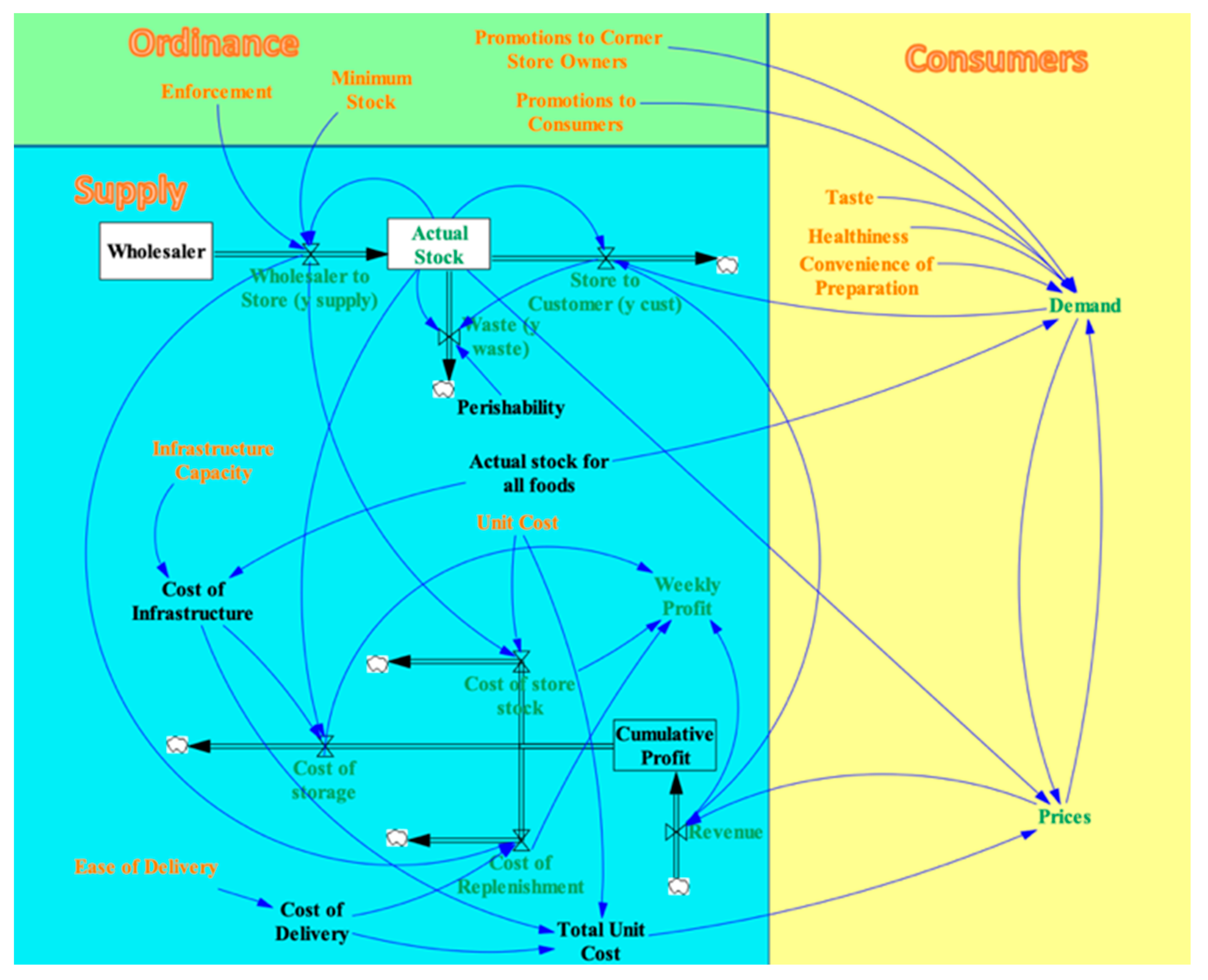
2.1.1. Step 1: Developing a Visual Model
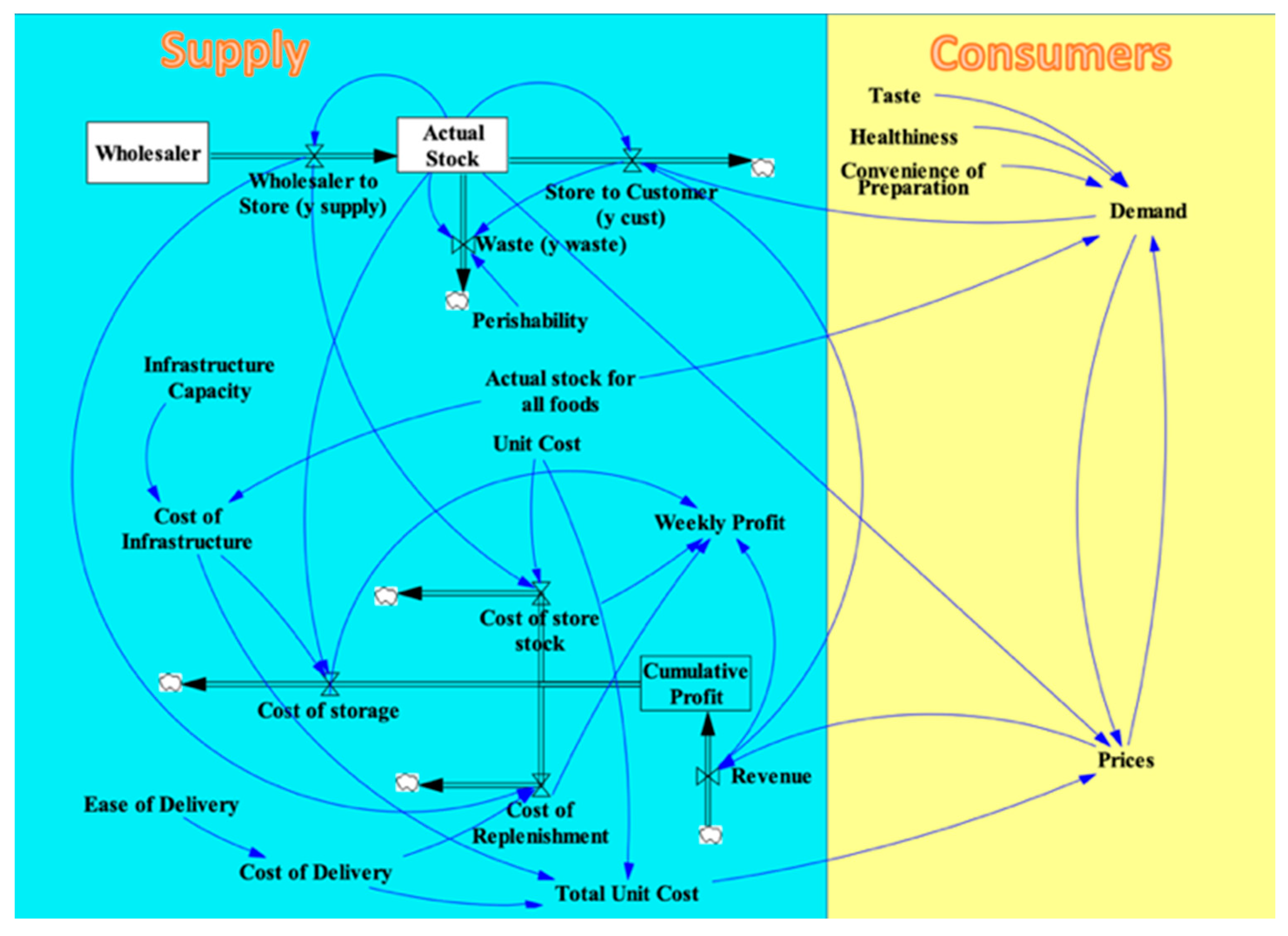
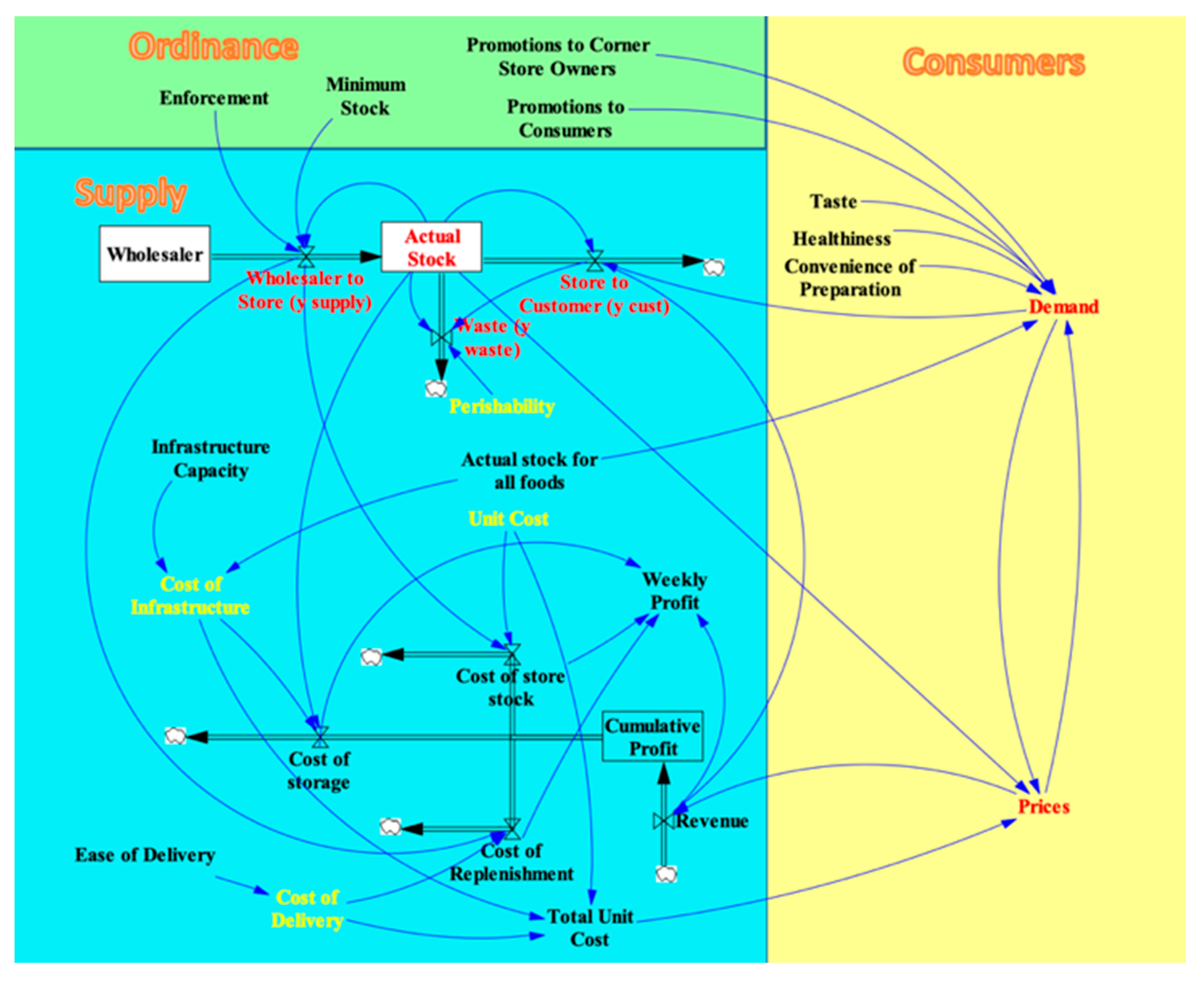
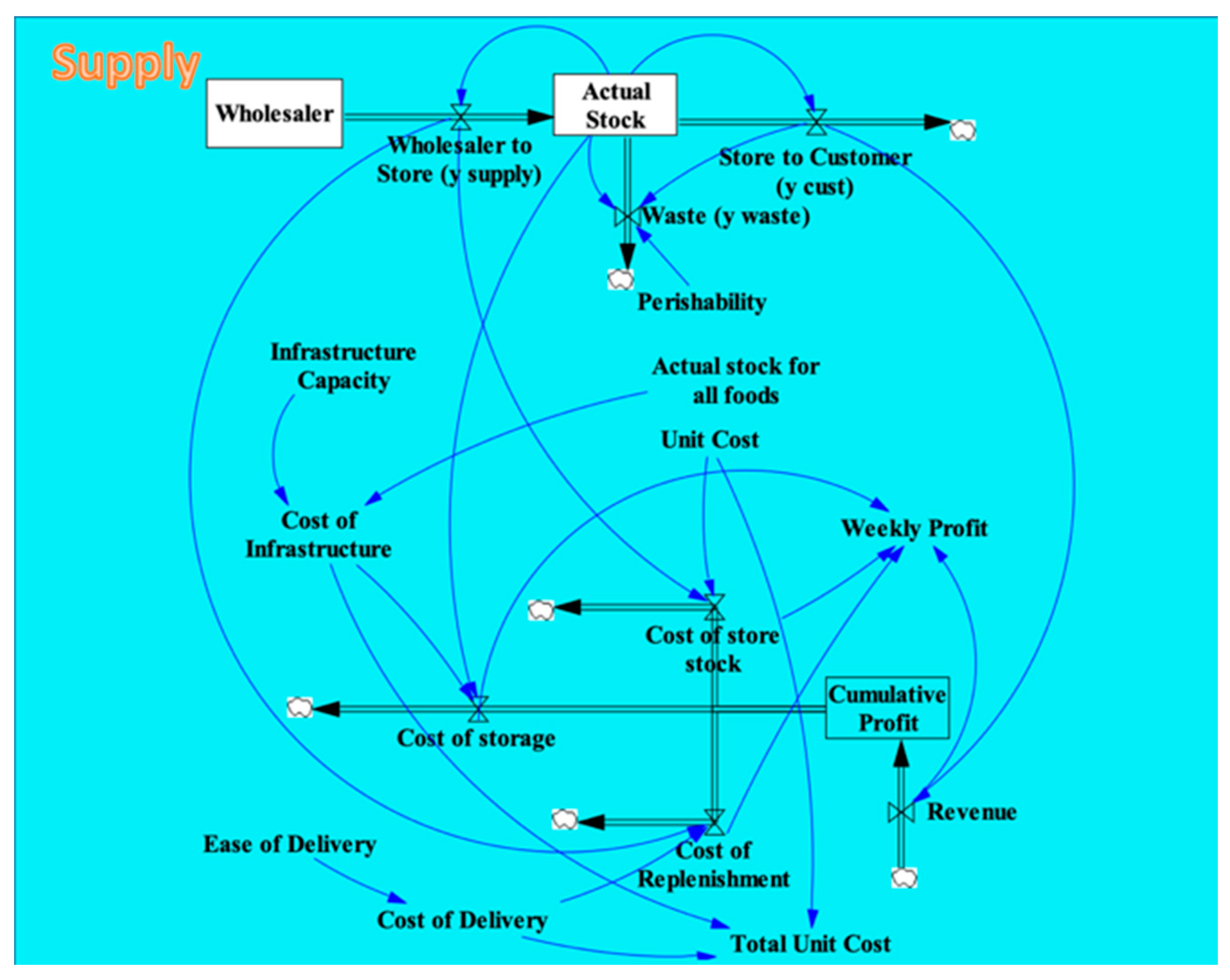
Retailer Dimension of the SFO Visual Model
Consumer Dimension of the SFO Visual Model
Ordinance Dimension of the SFO Visual Model
2.1.2. Step 2: Developing the Mathematical Model
- (y) flows of tomatoes (tomatoes/(time step))
- (s) stocks of tomatoes (tomatoes)
- (c) unit costs associated with tomatoes (dollars/tomato)
- (m) flows of money (dollars/(time step))
- (x) data inputs rated on a scale from 1 to 5
- (p) slope and intersection parameters for each equation found by the data processing techniques described in Section 2.3
2.2. Data Collection to Parameterize the Model
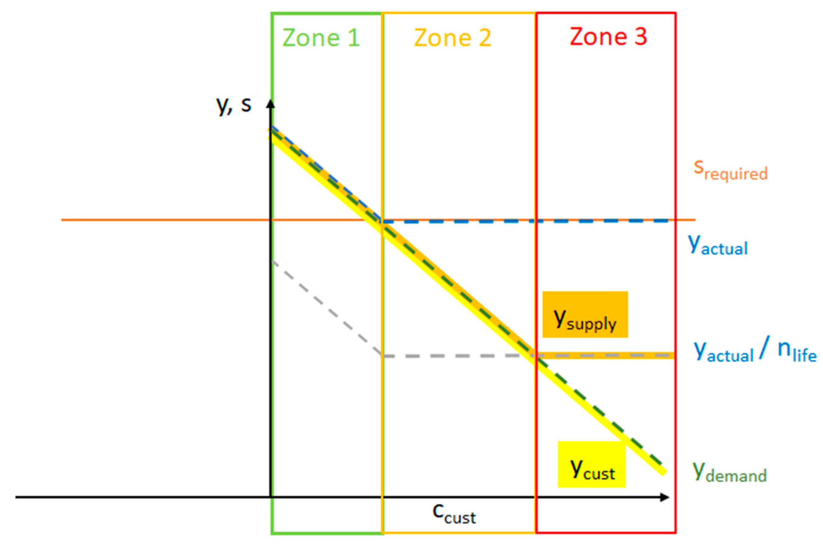
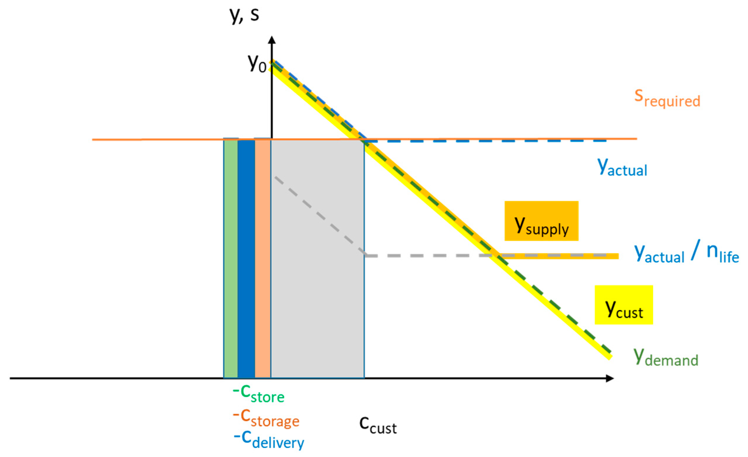
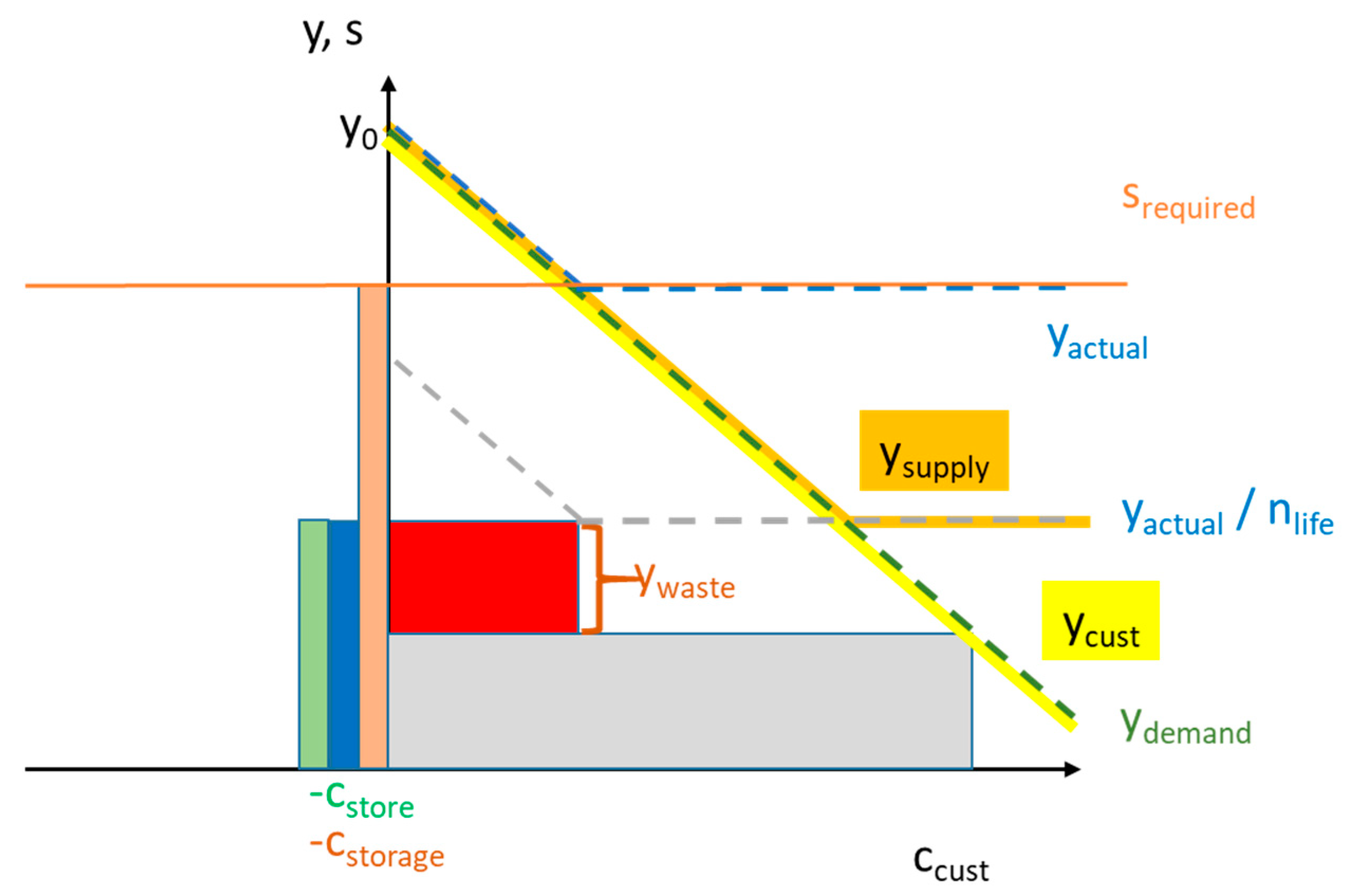
2.3. Data Processing
- The unit delivery cost is 5% of the price [53].
- The unit storage cost is 10% of the price plus the effect of the Actual Stock for All Foods variable.
- The maximum price is 200% of the average price and represents when there is no demand for the food because the price is too high.
2.3.1. Linear Regression to Parameterize the SD Equations
2.3.2. Demand Projection to Prepare Survey Data for Multi-Objective Linear Regression
2.3.3. Multi-Objective Linear Regression to Parameterize the SD Equations
2.4. Simulation Method
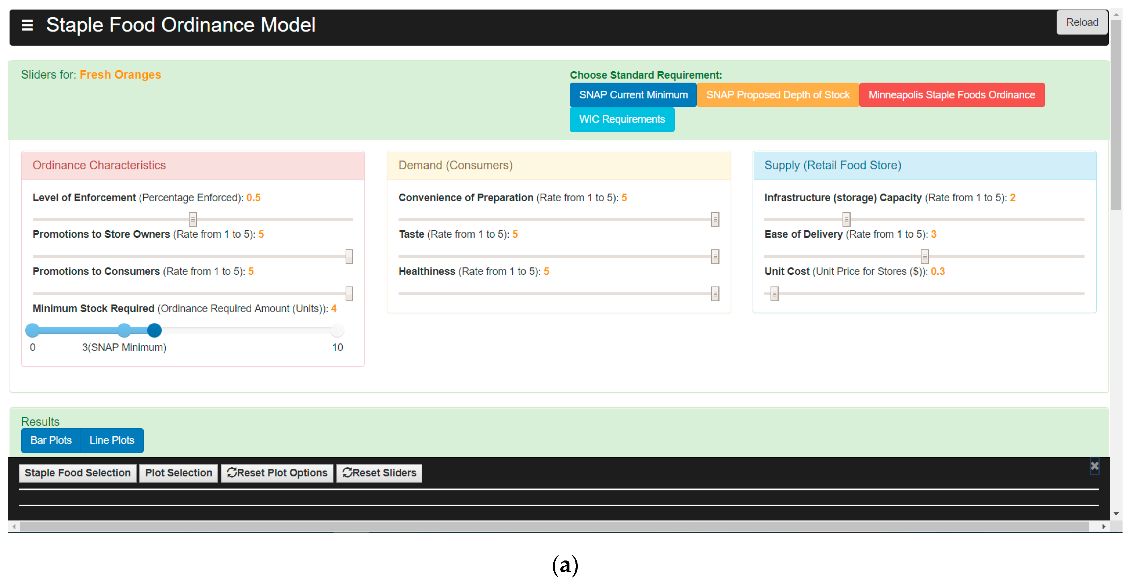
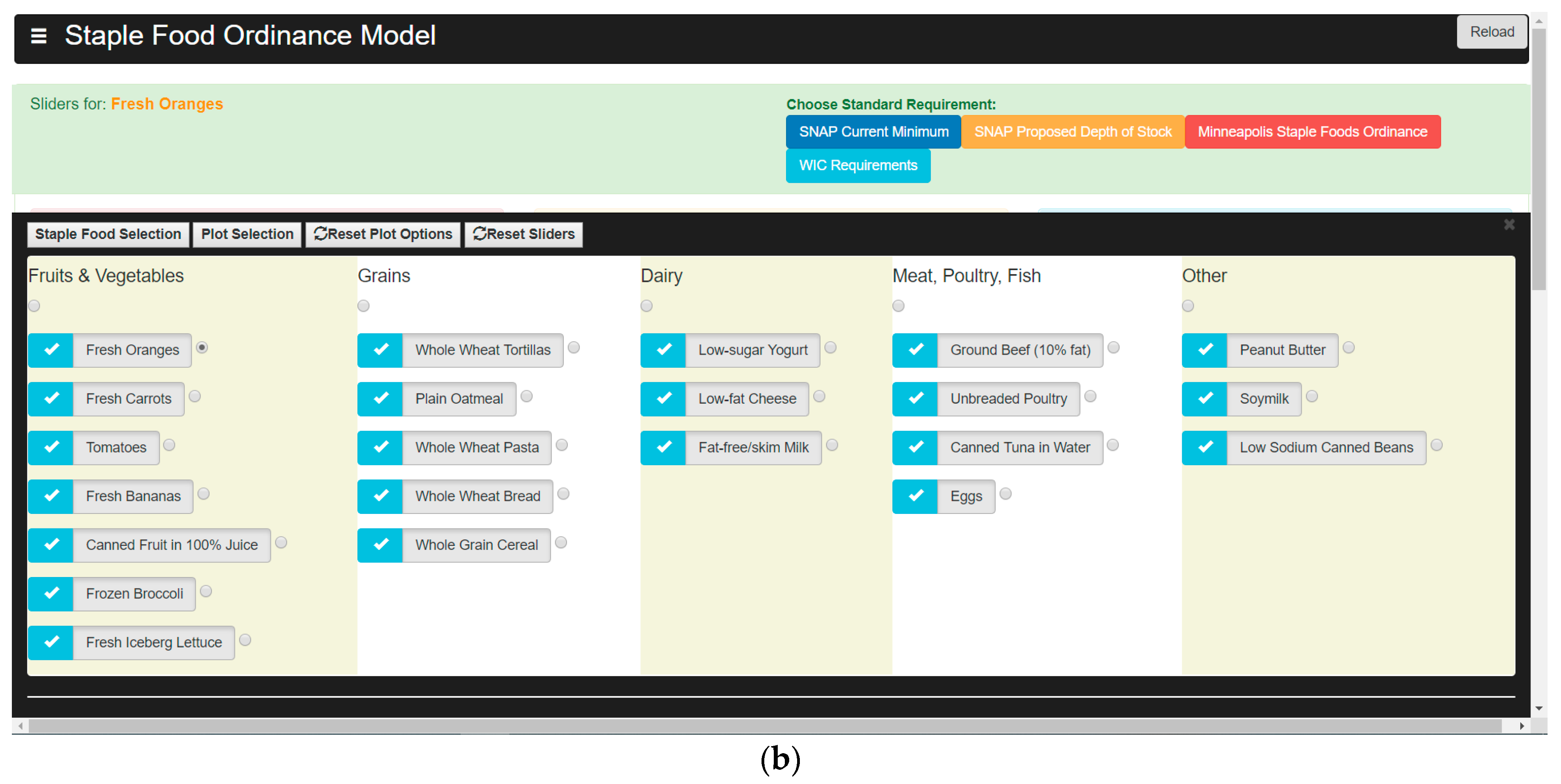
- Input Variables, which users enter values for before running the simulation. These variables allow users to adapt the model for their specific environment. These variables are orange in Figure 5.
- Result Variables, which the simulation reports values for once it has finished. These variables allow users to see how changes to input variables affect the success of the corner store. These variables are green in Figure 5.
2.4.1. Pre-Simulation Profit Maximization
2.4.2. Simulation Runs
2.4.3. User Interface (UI)
3. Results
4. Discussion
5. Conclusions
Supplementary Materials
Author Contributions
Funding
Institutional Review Board Statement
Informed Consent Statement
Data Availability Statement
Conflicts of Interest
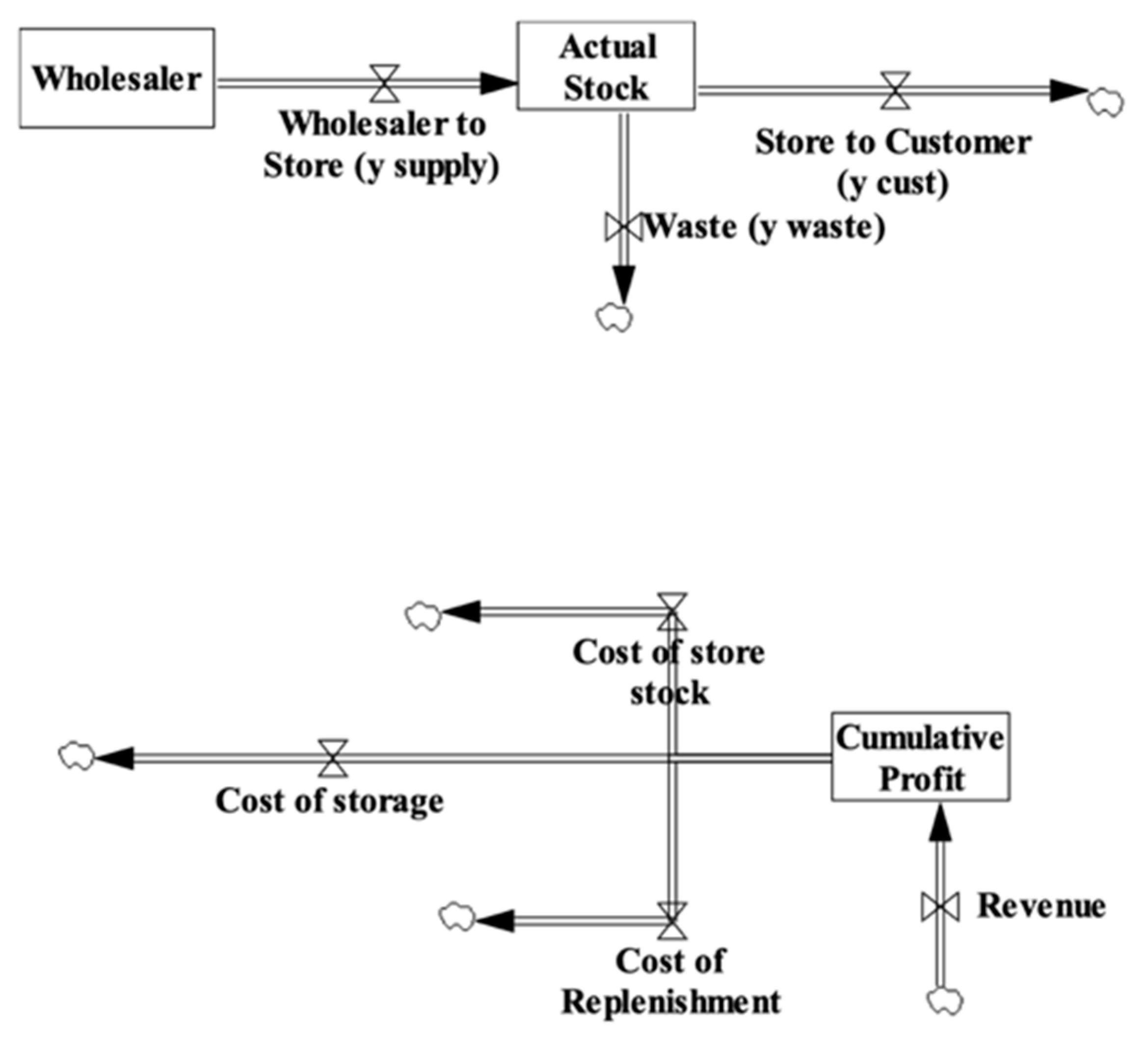
Appendix A. SD Mathematical Equations
- ysupply (units/week): Wholesaler to Store, the amount of this food that the wholesaler supplies to the store each week.
- srequired (units): Minimum Stock of this food as required by the ordinance.
- xenforcement (percentage): Enforcement of the ordinance by the government.
- yactual_end (units): Actual Stock of this food in the store at the end of the week.
- ydemand (units/week): Demand for this food by the store’s customers each week.
- yactual (units): Actual Stock of this food in the store at the beginning of the week.
- yactual_all (units): Actual Stock for All Foods in the corner store.
- yactual_all-food (units): Actual Stock in the store of the specific food (j) in time step (i).
- xtraining (scale 1–5): Promotion to Store Owner (Training, for example), a rating of the incentives the ordinance provides to promote store compliance.
- xsignage (scale 1–5): Promotion to Consumer (Signage, for example), a rating of the incentives the ordinance provides to encourage consumers to purchase staple foods at the store.
- xconvenience (scale 1–5): Convenience of Preparation, a rating of how easy the food is to prepare
- xtaste (scale 1–5): Taste, a rating of how good the food tastes
- xhealthiness (scale 1–5): Healthiness, a rating of how healthy the food is
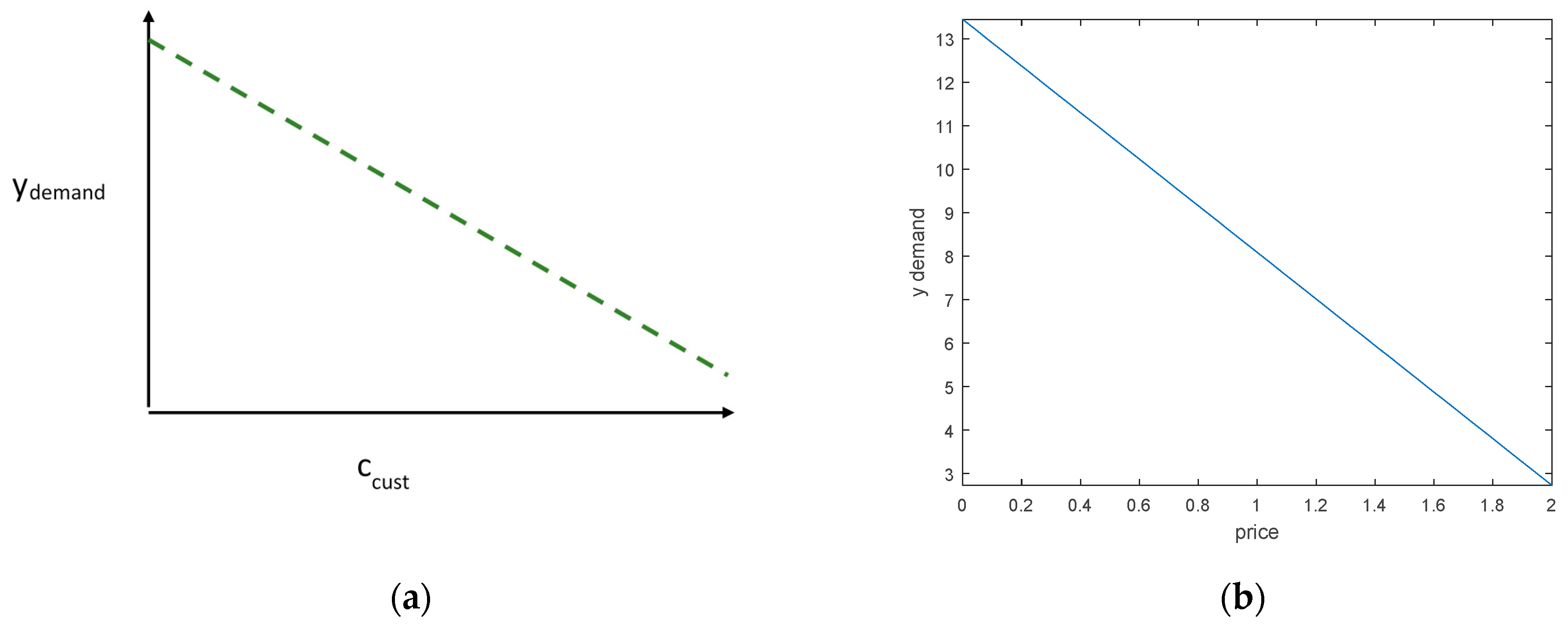
- ccust ($/unit): Price for customers to purchase one unit of this food from the store.
- p1–p6: Parameters for the demand equation found by running multi-objective linear regression on the data.
- p7: Slope of the Demand Curve based on price-demand data.
- p8: Parameter for the Actual Stock of All Foods that affects the demand for each food.
- ycust (units/week): Store to Customers, the amount of food purchased from the store by customers each week.
- ywaste (units/week): Waste, the amount of food wasted by the store each week.
- p9: Perishability, the shelf life of each food.
- cdelivery ($/unit): Cost of Delivery, the average cost to deliver a unit of food to the store from the wholesaler.
- xdelivery (scale 1–5): Ease of Delivery, a rating of how easy it is to deliver the food to the store from the wholesaler.
- p10: Intersection parameter for the Cost of Delivery equation found by running linear regression on store owner data.
- p11: Slope parameter for the Cost of Delivery equation found by running linear regression on store owner data.
- cstorage ($/unit): Cost of Storage, the cost to store a unit of food in the store, includes the cost of shelf space, refrigeration, electricity, and other overhead costs.
- sinfra (scale 1–5): Infrastructure Capacity, a rating that measures the available space in the store to store food.
- p12: Intersection parameter for the Cost of Storage equation found by running linear regression on store owner data.
- p13: Slope parameter for the Cost of Storage equation found by running linear regression on store owner data.
- p14: Parameter for the Actual Stock of All Foods that affects the unit cost of storage for each food.
- ctotal ($/unit): Total Unit Cost for the corner store to purchase the food from the wholesaler, including supply, delivery, and storage costs.
- cstore ($/unit): Cost of Store Stock, the cost for the corner store to purchase a unit of food from the wholesaler.
- mprofit ($/week): Weekly Profit, the net amount of money the store earns after deducting operating costs.
- mstorage ($/week): Weekly Cost of Storage to store food in the corner store.
- msupply ($/week): Weekly Cost of Store Stock to purchase food from the wholesaler.
- mdelivery ($/week): Weekly Cost of Replenishment to deliver food to the corner store.
- mcust ($/week): Weekly Revenue, the gross amount of money the store earns from customer purchases before deducting operating costs.
Appendix B. Economic Model

= (a × (y0 − ydemand) − cstore − cdelivery) × ydemand − cstorage × srequired,

= (a × (y0 − ydemand)) × ydemand − (cstore + cdelivery) × ysupply − cstorage × srequired,
Appendix C. Profit Maximization Algorithm
- Starting from zero, increase the price to the maximum price over n equal price-steps. Here, n was set to be 50 price-steps and a was set to be 2. The step size was determined using the equations below.pricemax = y0 × a,where,pricestep = (pricemax)/n,
- pricemax ($): The maximum price, defined as 2 times the average price . This value is also the demand curve’s intersection with the x axis, representing the price when there is zero demand.
- pricestep ($): The increase in price during each price-step of the profit maximization algorithm.
- For each price-step, run the SD equation set for 60 time-steps until the value of the total profit converges.
- Compare the values of the total profit for each price-step.
- Save the index of the price-step that result in the highest profit. This index locates the column that will be used for all of the input variable matrices in that time step when the simulation is run.
Appendix D. Demand Projection Equations
- rdesired_storeOwner (scale 1–5): The survey rating of either the store owner’s preferred amount of stock or the store owner’s perceived consumer demand, whichever is smaller in the store owners’ dataset.
- demandstoreowner (units/week): The quantity of a particular food that the store owner demands at a particular store in the store owners’ dataset
- μdemand_storeOwner (units/week): The mean value of store owner demand across all corner stores for a particular food.
- demandconsumer (units/week): The amount of a particular food that consumers demand at a particular store in the consumers’ dataset.
- μdemand_consumer (units/week): The mean value of consumer demand across all corner stores for a particular food.
- dmdproj (units/week): Projected demand data used for linear regression.
Appendix E. Detailed Numerical Results from SFO Simulations

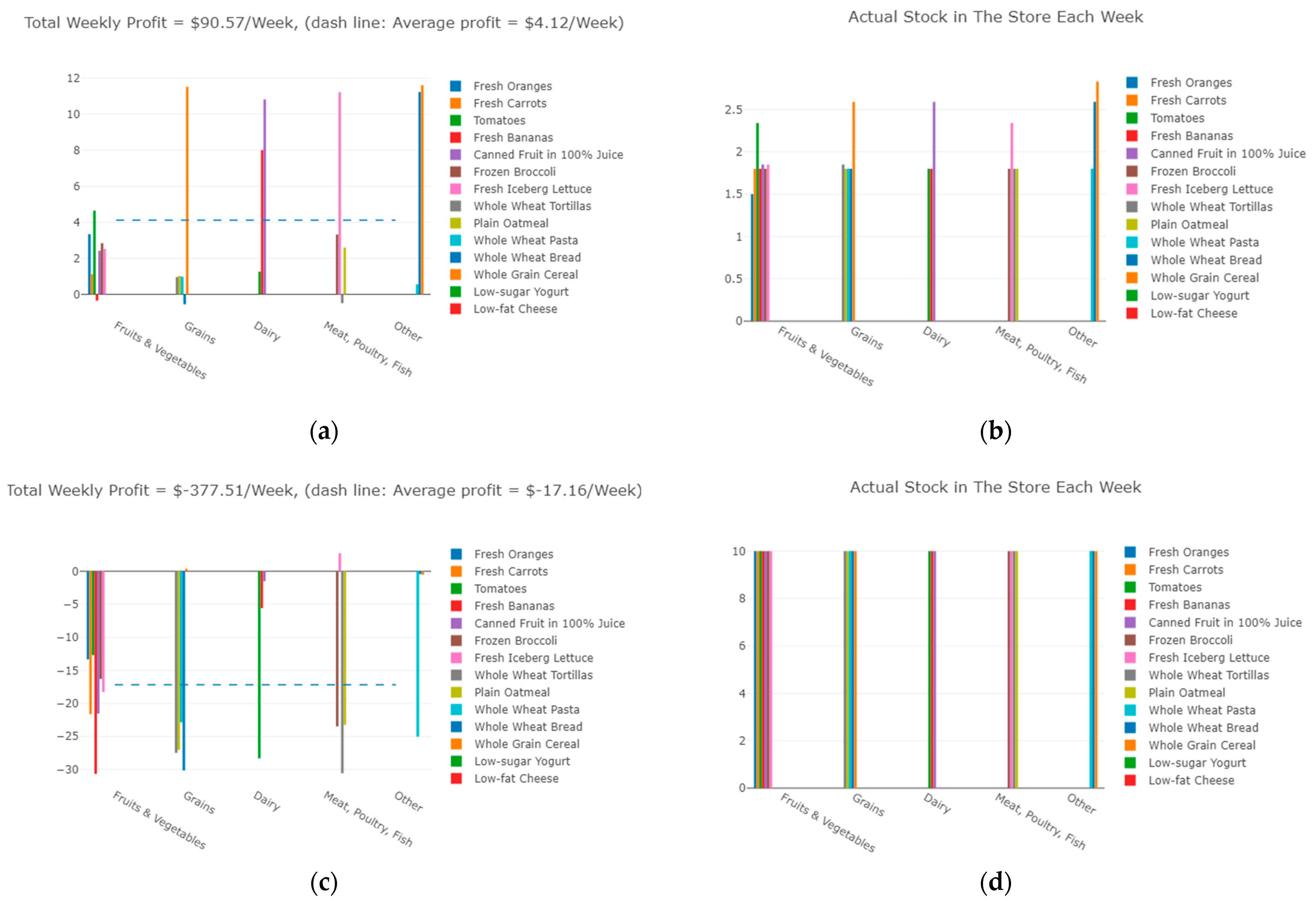
| Type of Food | Weekly Profit | Actual Stock of Food (Units of Food per Week) | Waste (Units of Food per Week) |
|---|---|---|---|
| Total | $90.57 | 43.93 | 0 |
| Average | $4.12 | 2.00 | 0 |
| Fresh Oranges | $3.34 | 1.50 | 0 |
| Fresh Carrots | $1.12 | 1.80 | 0 |
| Tomatoes | $4.65 | 2.34 | 0 |
| Fresh Bananas | −$0.35 | 1.80 | 0 |
| Canned Fruit | $2.42 | 1.85 | 0 |
| Frozen Broccoli | $2.84 | 1.80 | 0 |
| Fresh Iceberg Lettuce | $2.52 | 1.85 | 0 |
| Whole Wheat Tortillas | $0.96 | 1.85 | 0 |
| Plain Oatmeal | $1.03 | 1.80 | 0 |
| Whole Wheat Pasta | $0.98 | 1.80 | 0 |
| Whole Wheat Bread | −$0.55 | 1.80 | 0 |
| Whole Grain Cereal | $11.52 | 2.59 | 0 |
| Low-Sugar Yogurt | $1.26 | 1.80 | 0 |
| Low-Fat Cheese | $8.01 | 1.80 | 0 |
| Fat-Free/Skim Milk | $10.82 | 2.59 | 0 |
| Ground Beef (10% fat) | $3.32 | 1.80 | 0 |
| Unbreaded Poultry | $11.22 | 2.34 | 0 |
| Canned Tuna | −$0.49 | 1.80 | 0 |
| Eggs | $2.60 | 1.80 | 0 |
| Peanut Butter | $0.55 | 1.80 | 0 |
| Soymilk | $11.23 | 2.59 | 0 |
| Canned Beans | $11.61 | 2.83 | 0 |
| Type of Food | Weekly Profit | Actual Stock of Food (Units of Food per Week) | Waste (Units of Food per Week) |
|---|---|---|---|
| Total | −$377.51 | 220 | 2.61 |
| Average | −$17.16 | 10 | 0.12 |
| Fresh Oranges | −$13.32 | 10 | 0.56 |
| Fresh Carrots | −$21.62 | 10 | 0.58 |
| Tomatoes | −$12.67 | 10 | 0.52 |
| Fresh Bananas | −$30.67 | 10 | 0.47 |
| Canned Fruit | −$21.53 | 10 | 0 |
| Frozen Broccoli | −$16.28 | 10 | 0 |
| Fresh Iceberg Lettuce | −$18.27 | 10 | 0 |
| Whole Wheat Tortillas | −$27.49 | 10 | 0 |
| Plain Oatmeal | −$27.04 | 10 | 0 |
| Whole Wheat Pasta | −$22.84 | 10 | 0 |
| Whole Wheat Bread | −$30.14 | 10 | 0 |
| Whole Grain Cereal | $0.37 | 10 | 0 |
| Low-Sugar Yogurt | −$28.32 | 10 | 0 |
| Low-Fat Cheese | −$5.60 | 10 | 0 |
| Fat-Free/Skim Milk | −$1.53 | 10 | 0 |
| Ground Beef (10% fat) | −$23.48 | 10 | 0 |
| Unbreaded Poultry | $2.72 | 10 | 0.48 |
| Canned Tuna | −$30.57 | 10 | 0 |
| Eggs | −$23.26 | 10 | 0 |
| Peanut Butter | −$25.02 | 10 | 0 |
| Soymilk | −$0.44 | 10 | 0 |
| Canned Beans | −$0.52 | 10 | 0 |
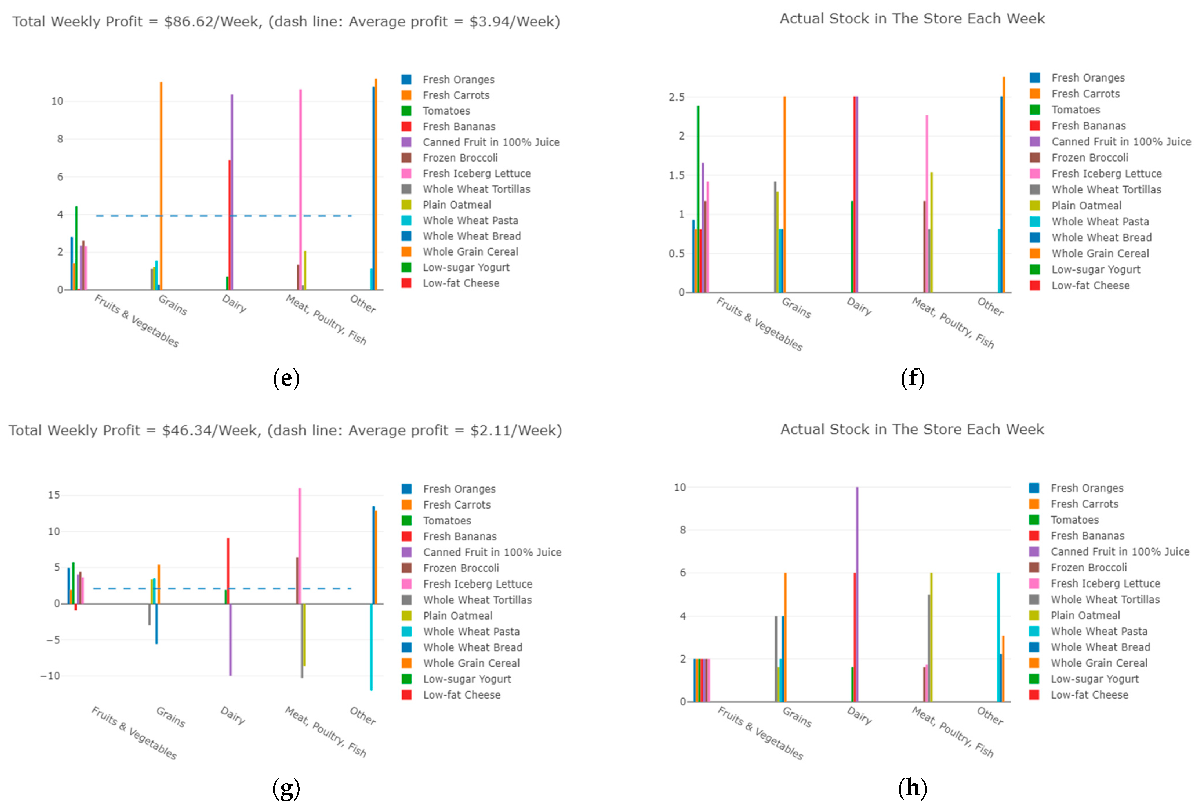
| Type of Food | Weekly Profit | Actual Stock of Food (Units of Food per Week) | Waste (Units of Food per Week) |
|---|---|---|---|
| Total | $86.62 | 34.09 | 0 |
| Average | $3.94 | 1.55 | 0 |
| Fresh Oranges | $2.81 | 0.93 | 0 |
| Fresh Carrots | $1.42 | 0.81 | 0 |
| Tomatoes | $4.45 | 2.39 | 0 |
| Fresh Bananas | $0.05 | 0.81 | 0 |
| Canned Fruit | $2.35 | 1.66 | 0 |
| Frozen Broccoli | $2.61 | 1.17 | 0 |
| Fresh Iceberg Lettuce | $2.33 | 1.42 | 0 |
| Whole Wheat Tortillas | $1.12 | 1.42 | 0 |
| Plain Oatmeal | $1.22 | 1.29 | 0 |
| Whole Wheat Pasta | $1.55 | 0.81 | 0 |
| Whole Wheat Bread | $0.28 | 0.81 | 0 |
| Whole Grain Cereal | $11.04 | 2.51 | 0 |
| Low-Sugar Yogurt | $0.70 | 1.17 | 0 |
| Low-Fat Cheese | $6.89 | 2.51 | 0 |
| Fat-Free/Skim Milk | $10.38 | 2.51 | 0 |
| Ground Beef (10% fat) | $1.34 | 1.17 | 0 |
| Unbreaded Poultry | $10.64 | 2.27 | 0 |
| Canned Tuna | $0.25 | 0.81 | 0 |
| Eggs | $2.07 | 1.54 | 0 |
| Peanut Butter | $1.14 | 0.81 | 0 |
| Soymilk | $10.78 | 2.51 | 0 |
| Canned Beans | $11.21 | 2.76 | 0 |
| Type of Food | Weekly Profit | Actual Stock of Food (Units of Food per Week) | Waste (Units of Food per Week) |
|---|---|---|---|
| Total | $46.34 | 74.91 | 0 |
| Average | $2.11 | 3.41 | 0 |
| Fresh Oranges | $4.95 | 2 | 0 |
| Fresh Carrots | $1.94 | 2 | 0 |
| Tomatoes | $5.71 | 2 | 0 |
| Fresh Bananas | −$0.89 | 2 | 0 |
| Canned Fruit | $4.02 | 2 | 0 |
| Frozen Broccoli | $4.40 | 2 | 0 |
| Fresh Iceberg Lettuce | $3.64 | 2 | 0 |
| Whole Wheat Tortillas | −$2.96 | 4 | 0 |
| Plain Oatmeal | $3.37 | 1.62 | 0 |
| Whole Wheat Pasta | $3.47 | 2 | 0 |
| Whole Wheat Bread | −$5.58 | 4 | 0 |
| Whole Grain Cereal | $5.40 | 6 | 0 |
| Low-Sugar Yogurt | $1.93 | 1.62 | 0 |
| Low-Fat Cheese | $9.10 | 6 | 0 |
| Fat-Free/Skim Milk | −$9.98 | 10 | 0 |
| Ground Beef (10% fat) | $6.42 | 1.62 | 0 |
| Unbreaded Poultry | $16.01 | 1.74 | 0 |
| Canned Tuna | −$10.31 | 5 | 0 |
| Eggs | −$8.64 | 6 | 0 |
| Peanut Butter | −$12.03 | 6 | 0 |
| Soymilk | $13.49 | 2.23 | 0 |
| Canned Beans | $12.89 | 3.08 | 0 |
References
- Flegal, K.M.; Carroll, M.D.; Kit, B.K.; Ogden, C.L. Prevalence of Obesity and Trends in the Distribution of Body Mass Index among US Adults, 1999–2010. JAMA 2012, 307, 491–497. [Google Scholar] [CrossRef] [Green Version]
- Falbe, J.; Thompson, H.R.; Becker, C.M.; Rojas, N.; McCulloch, C.E.; Madsen, K.A. Impact of the Berkeley Excise Tax on Sugar-Sweetened Beverage Consumption. Am. J. Public Health 2016, 106, 1865–1871. [Google Scholar] [CrossRef] [PubMed]
- Claro, R.M.; Levy, R.B.; Popkin, B.; Monteiro, C.A. Sugar-Sweetened Beverage Taxes in Brazil. Am. J. Public Health 2012, 102, 178–183. [Google Scholar] [CrossRef] [PubMed]
- Rajagopal, S.; Barnhill, A.; Sharfstein, J.M. The evidence—and acceptability—of taxes on unhealthy foods. Isr. J. Health Policy Res. 2018, 7, 68. [Google Scholar] [CrossRef]
- Franck, C.; Grandi, S.M.; Eisenberg, M.J. Taxing Junk Food to Counter Obesity. Am. J. Public Health 2013, 103, 1949–1953. [Google Scholar] [CrossRef] [PubMed]
- National Conference of State Legislatures. Available online: https://www.ncsl.org/research/agriculture-and-rural-development/urban-agriculture-state-legislation.aspx (accessed on 15 January 2020).
- Elbel, B.; Mijanovich, T.; Kiszko, K.; Abrams, C.; Cantor, J.; Dixon, L.B. The Introduction of a Supermarket via Tax-Credits in a Low-Income Area: The Influence on Purchasing and Consumption. Am. J. Health Promot. 2017, 31, 59–66. [Google Scholar] [CrossRef]
- Andreyeva, T.; Long, M.; Brownell, K.D. The Impact of Food Prices on Consumption: A Systematic Review of Research on the Price Elasticity of Demand for Food. Am. J. Public Health 2010, 100, 216–222. [Google Scholar] [CrossRef]
- Green, R.; Cornelsen, L.; Dangour, A.; Turner, R.; Shankar, B.; Mazzocchi, M.; Smith, R. The effect of rising food prices on food consumption: Systematic review with meta-regression. BMJ 2013, 346, f3703. [Google Scholar] [CrossRef] [Green Version]
- Song, H.-J.; Gittelsohn, J.; Kim, M.; Suratkar, S.; Sharma, S.; Anliker, J. A corner store intervention in a low-income urban community is associated with increased availability and sales of some healthy foods. Public Health Nutr. 2009, 12, 2060–2067. [Google Scholar] [CrossRef] [Green Version]
- Gittelsohn, J.; Song, H.-J.; Suratkar, S.; Kumar, M.B.; Henry, E.G.; Sharma, S.; Mattingly, M.; Anliker, J.A. An Urban Food Store Intervention Positively Affects Food-Related Psychosocial Variables and Food Behaviors. Health Educ. Behav. 2009, 37, 390–402. [Google Scholar] [CrossRef]
- Gittelsohn, J.; Suratkar, S.; Song, H.-J.; Sacher, S.; Rajan, R.; Rasooly, I.R.; Bednarek, E.; Sharma, S.; Anliker, J.A. Process Evaluation of Baltimore Healthy Stores: A Pilot Health Intervention Program With Supermarkets and Corner Stores in Baltimore City. Health Promot. Pract. 2009, 11, 723–732. [Google Scholar] [CrossRef]
- Gittelsohn, J.; Kim, E.M.; He, S.; Pardilla, M. A Food Store–Based Environmental Intervention Is Associated with Reduced BMI and Improved Psychosocial Factors and Food-Related Behaviors on the Navajo Nation. J. Nutr. 2013, 143, 1494–1500. [Google Scholar] [CrossRef] [PubMed]
- Townshend, T.; Lake, A. Obesogenic environments: Current evidence of the built and food environments. Perspect. Public Health 2017, 137, 38–44. [Google Scholar] [CrossRef] [Green Version]
- Morland, K.; Wing, S.; Roux, A.D. The Contextual Effect of the Local Food Environment on Residents’ Diets: The Atherosclerosis Risk in Communities Study. Am. J. Public Health 2002, 92, 1761–1768. [Google Scholar] [CrossRef] [PubMed]
- Gordon-Larsen, P. Food Availability/Convenience and Obesity. Adv. Nutr. 2014, 5, 809–817. [Google Scholar] [CrossRef] [PubMed]
- Hill, J.O.; Peters, J.C. Environmental Contributions to the Obesity Epidemic. Science 1998, 280, 1371–1374. [Google Scholar] [CrossRef] [PubMed]
- Franco, M.; Roux, A.V.; Nettleton, J.A.; Lazo, M.; Brancati, F.; Caballero, B. Availability of healthy foods and dietary patterns: The Multi-Ethnic Study of Atherosclerosis Neighborhood characteristics and availability of healthy foods in Baltimore. Am. J. Clin. Nutr. 2009, 89, 897–904. [Google Scholar] [CrossRef] [Green Version]
- Beydoun, M.A.; Wang, Y. How do socio-economic status, perceived economic barriers and nutritional benefits affect quality of dietary intake among US adults? Eur. J. Clin. Nutr. 2007, 62, 303–313. [Google Scholar] [CrossRef]
- Popkin, B.M.; Duffey, K.J.; Gordon-Larsen, P. Environmental influences on food choice, physical activity and energy balance. Physiol. Behav. 2005, 86, 603–613. [Google Scholar] [CrossRef]
- Cohen, D.A.; Inagami, S.; Finch, B. The built environment and collective efficacy. Health Place 2008, 14, 198–208. [Google Scholar] [CrossRef] [Green Version]
- Dhakal, C.; Khadka, S. Heterogeneities in Consumer Diet Quality and Health Outcomes of Consumers by Store Choice and Income. Nutrients 2021, 13, 1046. [Google Scholar] [CrossRef]
- Gamba, R.J.; Schuchter, J.; Rutt, C.; Seto, E.Y.W. Measuring the Food Environment and its Effects on Obesity in the United States: A Systematic Review of Methods and Results. J. Community Health 2014, 40, 464–475. [Google Scholar] [CrossRef]
- Zenk, S.N.; Odoms-Young, A.M.; Dallas, C.; Hardy, E.; Watkins, A.; Hoskins-Wroten, J.; Holland, L. “You Have to Hunt for the Fruits, the Vegetables”: Environmental Barriers and Adaptive Strategies to Acquire Food in a Low-Income African American Neighborhood. Health Educ. Behav. 2011, 38, 282–292. [Google Scholar] [CrossRef] [Green Version]
- Zenk, S.N.; Schulz, A.J.; Israel, B.A.; James, S.A.; Bao, S.; Wilson, M.L. Fruit and vegetable access differs by community racial composition and socioeconomic position in Detroit, Michigan. Ethn. Dis. 2006, 16, 275–280. [Google Scholar] [PubMed]
- Lee-Kwan, S.H.; Kumar, G.; Ayscue, P.; Santos, M.; McGuire, L.C.; Blanck, H.M.; Nua, M.T. Healthful food availability in stores and restaurants—American Samoa, 2014. MMWR Morb. Mortal. Wkly. Rep. 2015, 64, 276–278. [Google Scholar] [PubMed]
- Bower, K.M.; Thorpe, R.J.; Rohde, C.; Gaskin, D.J. The intersection of neighborhood racial segregation, poverty, and urbanicity and its impact on food store availability in the United States. Prev. Med. 2014, 58, 33–39. [Google Scholar] [CrossRef] [PubMed] [Green Version]
- Powell, L.M.; Slater, S.; Mirtcheva, D.; Bao, Y.; Chaloupka, F.J. Food store availability and neighborhood characteristics in the United States. Prev. Med. 2007, 44, 189–195. [Google Scholar] [CrossRef] [PubMed]
- Caspi, C.E.; Pelletier, J.E.; Harnack, L.J.; Erickson, D.J.; Laska, M. Differences in healthy food supply and stocking practices between small grocery stores, gas-marts, pharmacies and dollar stores. Public Health Nutr. 2016, 19, 540–547. [Google Scholar] [CrossRef] [Green Version]
- Escaron, A.L.; Meinen, A.M.; Nitzke, S.A.; Martinez-Donate, A.P. Supermarket and Grocery Store–Based Interventions to Promote Healthful Food Choices and Eating Practices: A Systematic Review. Prev. Chronic Dis. 2013, 10, E50. [Google Scholar] [CrossRef] [Green Version]
- Michimi, A.; Wimberly, M.C. Associations of supermarket accessibility with obesity and fruit and vegetable consumption in the conterminous United States. Int. J. Health Geogr. 2010, 9, 49. [Google Scholar] [CrossRef] [Green Version]
- Gustafson, A.; Lewis, S.; Perkins, S.; Wilson, C.; Buckner, E.; Vail, A. Neighbourhood and consumer food environment is associated with dietary intake among Supplemental Nutrition Assistance Program (SNAP) participants in Fayette County, Kentucky. Public Health Nutr. 2013, 16, 1229–1237. [Google Scholar] [CrossRef] [Green Version]
- Grundy, S.M. Multifactorial causation of obesity: Implications for prevention. Am. J. Clin. Nutr. 1998, 67, 563S–572S. [Google Scholar] [CrossRef] [PubMed]
- Ang, Y.N.; Wee, B.S.; Poh, B.K.; Ismail, M.N. Multifactorial Influences of Childhood Obesity. Curr. Obes. Rep. 2013, 2, 10–22. [Google Scholar] [CrossRef]
- Chalk, M.B. Obesity: Addressing a multifactorial disease. Case Manag. 2004, 15, 47–49. [Google Scholar] [CrossRef]
- Lee, B.Y.; Bartsch, S.M.; Mui, Y.; Haidari, L.A.; Spiker, M.L.; Gittelsohn, J. A systems approach to obesity. Nutr. Rev. 2017, 75 (Suppl. 1), 94–106. [Google Scholar] [CrossRef] [PubMed]
- Gittelsohn, J.; Mui, Y.; Adam, A.; Lin, S.; Kharmats, A.; Igusa, T.; Lee, B.Y. Incorporating Systems Science Principles into the Development of Obesity Prevention Interventions: Principles, Benefits, and Challenges. Curr. Obes. Rep. 2015, 4, 174–181. [Google Scholar] [CrossRef] [Green Version]
- Mui, Y.; Lee, B.Y.; Adam, A.; Kharmats, A.Y.; Budd, N.; Nau, C.; Gittelsohn, J. Healthy versus Unhealthy Suppliers in Food Desert Neighborhoods: A Network Analysis of Corner Stores’ Food Supplier Networks. Int. J. Environ. Res. Public Health 2015, 12, 15058–15074. [Google Scholar] [CrossRef] [Green Version]
- Kim, M.; Budd, N.; Batorsky, B.; Krubiner, C.; Manchikanti, S.; Waldrop, G.; Trude, A.; Gittelsohn, J. Barriers to and Facilitators of Stocking Healthy Food Options: Viewpoints of Baltimore City Small Storeowners. Ecol. Food Nutr. 2017, 56, 17–30. [Google Scholar] [CrossRef] [PubMed]
- Laska, M.N.; Borradaile, K.E.; Tester, J.; Foster, G.D.; Gittelsohn, J. Healthy food availability in small urban food stores: A comparison of four US cities. Public Health Nutr. 2009, 13, 1031–1035. [Google Scholar] [CrossRef] [Green Version]
- City of Passaic, NJ. Available online: https://ecode360.com/32444965 (accessed on 14 January 2020).
- Laska, M.N.; Caspi, C.E.; Lenk, K.; Moe, S.G.; Pelletier, J.E.; Harnack, L.J.; Erickson, D.J. Evaluation of the first U.S. staple foods ordinance: Impact on nutritional quality of food store offerings, customer purchases and home food environments. Int. J. Behav. Nutr. Phys. Act. 2019, 16, 1–20. [Google Scholar] [CrossRef] [PubMed] [Green Version]
- Budd, N.; Cuccia, A.; Jeffries, J.K.; Prasad, D.; Frick, K.D.; Powell, L.; Katz, F.A.; Gittelsohn, J. B’More Healthy: Retail Rewards--design of a multi-level communications and pricing intervention to improve the food environment in Baltimore City. BMC Public Health 2015, 15, 283. [Google Scholar] [CrossRef] [Green Version]
- Lee-Kwan, S.H.; Goedkoop, S.; Yong, R.; Batorsky, B.; Hoffman, V.; Jeffries, J.; Hamouda, M.; Gittelsohn, J. Development and implementation of the Baltimore healthy carry-outs feasibility trial: Process evaluation results. BMC Public Health 2013, 13, 638. [Google Scholar] [CrossRef] [Green Version]
- Gittelsohn, J.; Steeves, E.A.; Mui, Y.; Kharmats, A.Y.; Hopkins, L.C.; Dennis, D. B’More Healthy Communities for Kids: Design of a multi-level intervention for obesity prevention for low-income African American children. BMC Public Health 2014, 14, 942. [Google Scholar] [CrossRef] [Green Version]
- Lee-Kwan, S.H.; Bleich, S.N.; Kim, H.; Colantuoni, E.; Gittelsohn, J. Environmental Intervention in Carryout Restaurants Increases Sales of Healthy Menu Items in a Low-Income Urban Setting. Am. J. Health Promot. 2015, 29, 357–364. [Google Scholar] [CrossRef]
- Gittelsohn, J.; Trude, A.C.; Poirier, L.; Ross, A.; Ruggiero, C.; Schwendler, T.; Steeves, E.A. The Impact of a Multi-Level Multi-Component Childhood Obesity Prevention Intervention on Healthy Food Availability, Sales, and Purchasing in a Low-Income Urban Area. Int. J. Environ. Res. Public Health 2017, 14, 1371. [Google Scholar] [CrossRef] [PubMed] [Green Version]
- Andersen, D.F.; Rich, E.; Macdonald, R. System Dynamics Applications to Public Policy. In System Dynamics. Encyclopedia of Complexity and Systems Science Series; Dangerfield, B., Ed.; Springer: New York, NY, USA, 2020; pp. 253–271. [Google Scholar] [CrossRef]
- Radzicki, M.J.; Taylor, R.A. Origin of System Dynamics: Jay W. Forrester and the History of System Dynamics. In U.S. Department of Energy’s Introduction to System Dynamics; 2008; Available online: https://web.nmsu.edu/~lang/files/mike.pdf (accessed on 23 October 2008).
- D’Angelo, H.; Suratkar, S.; Song, H.-J.; Stauffer, E.; Gittelsohn, J. Access to food source and food source use are associated with healthy and unhealthy food-purchasing behaviours among low-income African-American adults in Baltimore City. Public Health Nutr. 2011, 14, 1632–1639. [Google Scholar] [CrossRef] [Green Version]
- Budd, N.; Jeffries, J.K.; Jones-Smith, J.; Kharmats, A.; McDermott, A.Y.; Gittelsohn, J. Store-directed price promotions and communications strategies improve healthier food supply and demand: Impact results from a randomized controlled, Baltimore City store-intervention trial. Public Health Nutr. 2017, 20, 3349–3359. [Google Scholar] [CrossRef] [Green Version]
- Nicholson, W.; Snyder, C. Microeconomic Theory: Basic Principles and Extensions, 11th ed.; South-Western: Mason, OH, USA, 2012; pp. 27–154. ISBN 978-111-1-52553-8. [Google Scholar]
- How to Properly Calculate the Operational Costs behind Your Product. Available online: https://www.easypost.com/blog/2017-05-04-how-to-properly-calculate-operational-costs-behind-your-product (accessed on 28 August 2019).
- Find Grocery Deals from Your Favorite Local Stores. Available online: https://www.mygrocerydeals.com/ (accessed on 24 January 2020).
- Groceries Delivered From Local Stores. Available online: https://www.instacart.com/ (accessed on 24 January 2020).
- Gittelsohn, J.; Poirier, L.; Zhu, S.; Igusa, T. Staple Food Ordinance Model (Version 1.4); Johns Hopkins University: Baltimore, MD, USA, 2019; (Mobile application); Available online: https://engineering.jhu.edu/tak/SFO/UI/index.html (accessed on 24 January 2020).
- Supplemental Nutrition Assistance Program (SNAP). Available online: https://www.fns.usda.gov/snap/supplemental-nutrition-assistance-program (accessed on 24 January 2020).
- Staple Foods Ordinance. Available online: http://www.minneapolismn.gov/health/living/eating/staple-foods (accessed on 24 January 2020).
- Special Supplemental Nutrition Program for Women, Infants, and Children (WIC). Available online: https://www.fns.usda.gov/wic (accessed on 24 January 2020).
- Retailer Eligibility—Clarification of Criterion A and Criterion B Requirements. Available online: https://www.fns.usda.gov/snap/retailer-eligibility-clarification-of-criterion (accessed on 14 July 2020).
- Enhancing Retailer Standards in the Supplemental Nutrition Assistance Program (SNAP). Available online: https://www.federalregister.gov/documents/2016/12/15/2016-29837/enhancing-retailer-standards-in-the-supplemental-nutrition-assistance-program-snap (accessed on 14 July 2020).
- Counting Carrots in Corner Stores: The Minneapolis Staple Foods Ordinance. Available online: https://www.healthypeople.gov/2020/law-and-health-policy/bright-spot/counting-carrots-in-corner-stores-the-minneapolis-staple-foods-ordinance (accessed on 14 July 2020).
- Hennessy, E.; Economos, C.D.; Hammond, R.A.; Sweeney, L.B.; Brukilacchio, L.; Chomitz, V.R.; Collins, J.; Nahar, E.; Rioles, N.; Allender, S.; et al. Integrating Complex Systems Methods to Advance Obesity Prevention Intervention Research. Health Educ. Behav. 2020, 47, 213–223. [Google Scholar] [CrossRef] [PubMed]
- Kasman, M.; Hammond, R.A.; Heuberger, B.; Mack-Crane, A.; Purcell, R.; Economos, C.; Swinburn, B.; Allender, S.; Nichols, M. Activating a Community: An Agent-Based Model of Romp & Chomp, a Whole-of-Community Childhood Obesity Intervention. Obesity 2019, 27, 1494–1502. [Google Scholar] [CrossRef]
- Lyneis, J.M.; (Department of Social Science and Policy Studies, Worcester Polytechnic Institute). Teaching Introductory Microeconomics Using System Dynamics: Reflections on an Experiment at WPI. Course description. 2003. Available online: https://proceedings.systemdynamics.org/2003/proceed/PAPERS/218.pdf (accessed on 14 July 2020).


| Score | Desired Amount of Stock |
|---|---|
| 1 | 0 units |
| 2 | 1–3 units |
| 3 | 4–6 units |
| 4 | 7–9 units |
| 5 | 10 units or more |
| SFO Name | Description | Required Minimum Stock | Enforcement |
|---|---|---|---|
| SNAP Minimum | Minimal stocking requirements required to accept SNAP benefits | Low | Moderate |
| SNAP Depth | Stocking requirements for a food store under the 2016 United States Department of Agriculture proposed enhanced depth of stock requirements | High | High |
| Minneapolis | Stocking requirements used by the Minneapolis SFO | Moderate | Low |
| WIC | Stocking requirements if the store participated in the WIC program as a vendor | Moderate to High | High |
Publisher’s Note: MDPI stays neutral with regard to jurisdictional claims in published maps and institutional affiliations. |
© 2021 by the authors. Licensee MDPI, Basel, Switzerland. This article is an open access article distributed under the terms and conditions of the Creative Commons Attribution (CC BY) license (https://creativecommons.org/licenses/by/4.0/).
Share and Cite
Zhu, S.; Mitsinikos, C.; Poirier, L.; Igusa, T.; Gittelsohn, J. Development of a System Dynamics Model to Guide Retail Food Store Policies in Baltimore City. Nutrients 2021, 13, 3055. https://doi.org/10.3390/nu13093055
Zhu S, Mitsinikos C, Poirier L, Igusa T, Gittelsohn J. Development of a System Dynamics Model to Guide Retail Food Store Policies in Baltimore City. Nutrients. 2021; 13(9):3055. https://doi.org/10.3390/nu13093055
Chicago/Turabian StyleZhu, Siyao, Cassandra Mitsinikos, Lisa Poirier, Takeru Igusa, and Joel Gittelsohn. 2021. "Development of a System Dynamics Model to Guide Retail Food Store Policies in Baltimore City" Nutrients 13, no. 9: 3055. https://doi.org/10.3390/nu13093055
APA StyleZhu, S., Mitsinikos, C., Poirier, L., Igusa, T., & Gittelsohn, J. (2021). Development of a System Dynamics Model to Guide Retail Food Store Policies in Baltimore City. Nutrients, 13(9), 3055. https://doi.org/10.3390/nu13093055