Scale- and Region-Dependence in Landscape-PM_2.5 Correlation: Implications for Urban Planning

Abstract

Under rapid urbanization, many cities in China suffer from serious fine particulate matter (PM_2.5) pollution. As the emission sources or adsorption sinks, land use and the corresponding landscape pattern unavoidably affect the concentration. However, the correlation varies with different regions and scales, leaving a significant gap for urban planning. This study clarifies the correlation with the aid of in situ and satellite-based spatial datasets over six urban agglomerations in China. Two coverage and four landscape indices are adopted to represent land use and landscape pattern. Specifically, the coverage indices include the area ratios of forest (F_PLAND) and built-up areas (C_PLAND). The landscape indices refer to the perimeter-area fractal dimension index (PAFRAC), interspersion and juxtaposition index (IJI), aggregation index (AI), Shannon’s diversity index (SHDI). Then, the correlation between PM_2.5 concentration with the selected indices are evaluated from supporting the potential urban planning. Results show that the correlations are weak with the in situ PM_2.5 concentration, which are significant with the regional value. It means that land use coverage and landscape pattern affect PM_2.5 at a relatively large scale. Furthermore, regional PM_2.5 concentration negatively correlate to F_PLAND and positively to C_PLAND (significance at p < 0.05), indicating that forest helps to improve air quality, while built-up areas worsen the pollution. Finally, the heterogeneous landscape presents positive correlation to the regional PM_2.5 concentration in most regions, except for the urban agglomeration with highly-developed urban (i.e., the Jing-Jin-Ji and Chengdu-Chongqing urban agglomerations). It suggests that centralized urbanization would be helpful for PM_2.5 pollution controlling by reducing the emission sources in most regions. Based on the results, the potential urban planning is proposed for controlling PM_2.5 pollution for each urban agglomeration.

1. Introduction

Fine particulate matter (PM_2.5), defined as the particles with aerodynamic diameter less than 2.5 $\mathsf{\mu }\mathrm{m}$, causes seriously adverse human health (i.e., respiratory infection, heart disease, and lung cancer) [1,2,3,4]. Under rapid urbanization, PM_2.5 pollution has become an extreme environmental and social problem in many developing countries (particularly of China), causing millions of premature mortalities [5,6,7]. To improve air quality, it calls for fully understanding in the physical mechanisms of PM_2.5 formulation and dispersion [8,9].

Several factors account for PM_2.5 concentration dynamics, with the most important one refer to the climate condition in the previous studies [10]. The direct explanation is that water-soluble species of PM_2.5 could be easily dissolved in water, resulting in a significant reduction in concentration in rainfall conditions [11,12]. Wind is another important climate factor, which helps to disperse and dilute PM_2.5 concentration [13]. Observation experiments demonstrated that, PM_2.5 would decrease by 20–35% with wind velocity is higher than 2 m/s [14]. The latest research revealed that global warming also plays a considerable effect with respect to PM_2.5 concentration through the direct or indirect radiative effects [15]. Essentially, climate condition answers the causes of PM_2.5 dispersion. However, it is still difficult to explain the mechanisms of formulation [16].

Anthropogenic emission sources or adsorption sinks, correlate to the land use change, determine the formation and dissipation of PM_2.5 [17,18,19]. Generally, resident, road and industry land in urban are main emission sources of PM_2.5 [20,21,22]. Meanwhile, crop combustion and coal heating in rural play increasing contribution to regional PM_2.5 concentration, particularly in North China [23,24]. By contrast, forest usually acts as the adsorption sink, which could significantly reduce the PM_2.5 concentration [25,26,27]. Due to the effects above, PM_2.5 concentration tends to present significant spatial variability over different land use [28,29,30].

In addition to the types, limited numbers of researchers found that the spatial pattern of land use, namely the landscape pattern, also strongly affects the PM_2.5 concentration by determining the distribution of emission sources and adsorption sinks. It is revealed that PM_2.5 concentration would reduce along roads because of the deposition of roadside trees [31,32]. It would also influence the dispersion of PM_2.5 by altering the local climate [33,34]. Furthermore, the area, number, centrality, and fragmentation of the landscape patches would also strongly affect the PM_2.5 concentration [35]. Landscape indices are usually used to quantify land use patterns, which provide a link between the physical landscape structure and land use form, functionality and process [36,37,38]. The indices could be further adopted to evaluate the influence of land use on environmental process. For example, Wu et al. [39] investigated the impact of urban landscape pattern on PM_2.5 pollution in Beijing. Weber et al. [40] used the indices to explain the outdoor traffic-induced noise and PM₁₀ patterns. Due to the divergence between landscape elements, the effect of the landscape pattern is much more complex when compared to that of land use types [41]. It would further result in various correlations between landscape with geographical processes over different scales and regions [42,43]. Clarifying the spatial correlation is essential for urban planning and air pollution control. However, relevant studies are still rare and the spatial correlation remains unclear, leading to great difficulty for understanding the physical mechanism of PM_2.5 dynamics and supporting urban planning.

From the introduction above, it could be summarized that landscape would affect the PM_2.5 concentration. However, the correlation remains unclear. This study aims to clarify the correlation over different typical regions in China. Results of this study would help to understand the physical mechanism of PM_2.5 concentration, but also to support land use planning.

2. Materials and Methods

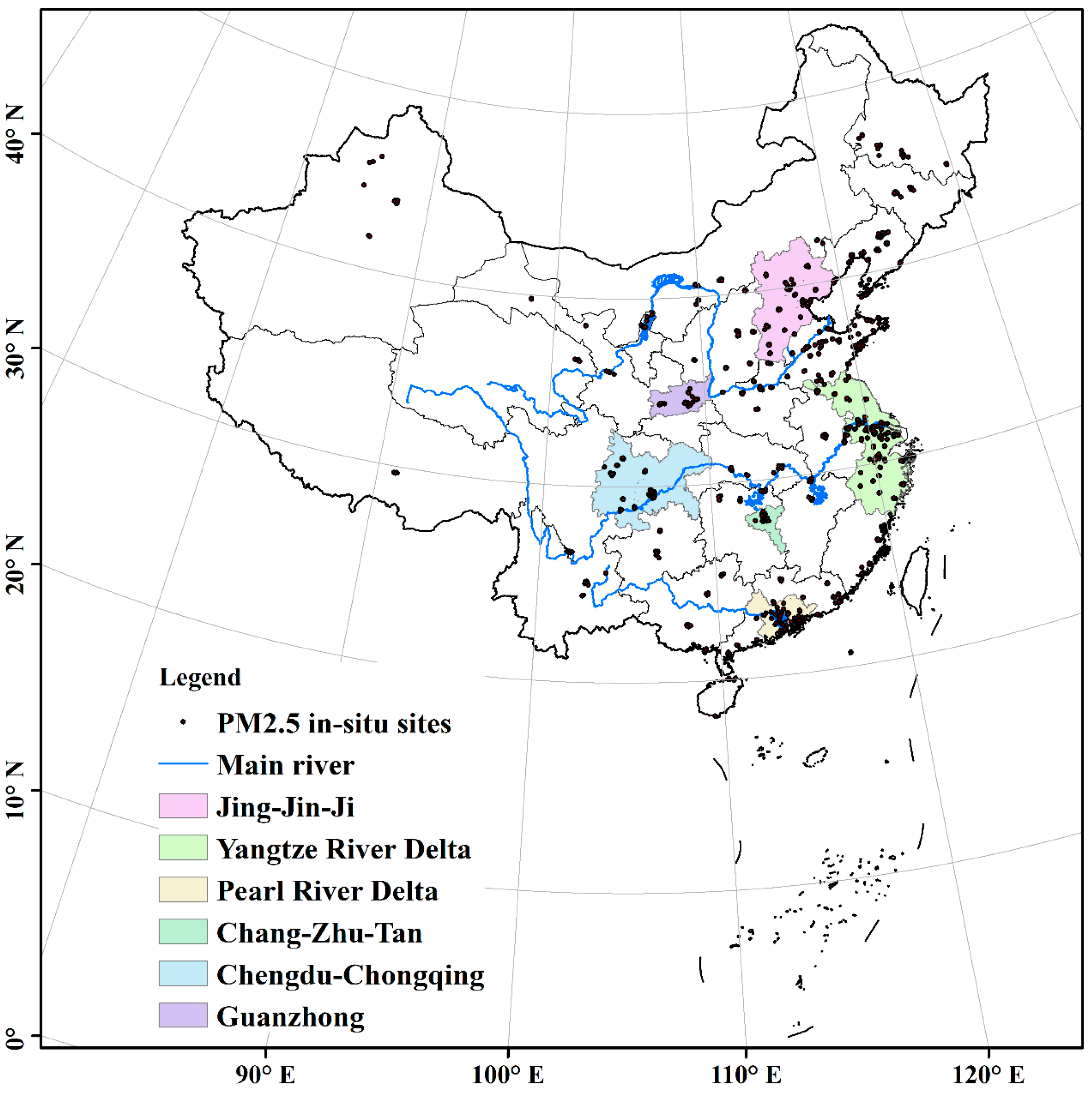
2.1. Study Area

In 2012, the Chinese government launched a National Plan on Air Pollution Control in Key Regions during the 12th Five-Year Plan (2011–2015) that set out, for the first-time, strict targets and measures to prevent and control air pollution in 13 key regions nationwide. The regions cover 14% of the area, 48% of the population, and 71% of the GDP of China, with the unit emissions are 2.9–3.6 times than that of the national mean. We selected six of them (Figure 1), including the Beijing-Tianjin-Hebei (Jing-Jin-Ji) region, the Yangtze River Delta, the Pearl River Delta, the Changsha-Zhuzhou-Xiangtan (Chang-Zhu-Tan), and the Chengdu-Chongqing and Guanzhong urban agglomerations, to investigate the correlation between PM_2.5 concentration and landscape pattern. The Jing-Jin-Ji region locates 113°04′–119°53′E and 36°01′–42°37′N, which covers 21.54 × 10⁴ km². PM_2.5 concentration reaches 97 μg/m³ in 2013 in this region. The Yangtze River Delta is one of the most developed regions in China. It covers about 21.17 × 10⁴ km² and is the largest estuary delta in China, with a population of 75 million. With the rapid urbanization, the Yangtze River Delta experienced serious air pollution in the last decades. The Pearl River Delta locates in the south of Guangdong province and covers 5.6 × 10⁴ km². The Chang-Zhu-Tan, Chengdu-Chongqing, and Guanzhong urban agglomerations are located in Central, Western, and Northern China with different pollution sources for PM_2.5 emissions, which helps to capture the spatial variability of PM_2.5 and the corresponding driving factors.

2.2. Data and Pre-Processing

2.2.1. Land Use

Land use data is used to generate landscape pattern and evaluate the correlation with PM_2.5 concentration. The data is obtained from the Geographical Information Monitoring Cloud Platform of China [44] in 2013. Six classes and 26 sub-classes of land use types are classified in this dataset with a spatial resolution of 30 m. Considering the dominant effects of land use on PM_2.5, we re-classify the types as farmland, forest, grassland, water, urban built-up, rural residential land, other built-up areas, and barren land.

2.2.2. In Situ PM_2.5 Concentration

The in situ PM_2.5 concentration is available from the China National Urban Air Quality Real-Time Publishing Platform Environmental Monitoring Center [45]. Hourly data is collected from 1 January to 31 December 2013, with the error within ±1.5 mg/m³. All missing or invalid data were removed, including the data of the same measurement repeatedly reported for several successive hours, significantly larger measurements, or measurements with less than 20 records a day. The quality-controlled data were then averaged in monthly and annual and prepared as the dependent variable for the following evaluation.

2.2.3. Satellite-Retrieved AOD Data

The ground observation data is difficult to reflect the spatial pattern of PM_2.5 concentration. Additionally, we select the satellite-retrieved aerosol optical depth (AOD) data for estimating the spatial PM_2.5. The daily level 2 (L2) AOD products (Collection 5.1) (10 km) from Terra and Aqua MODIS (Moderate Resolution Imaging Spectroradiometer) were downloaded from the Atmospheric Archive and Distribution System [46]. To eliminate the uncertainty originating from the product, only the AOD data with the best quality assurance was employed. To reduce the negative influence of cloud, we fitted a linear regression to combine the data sets of Terra AOD (MOD04) and the Aqua AOD (MYD04). We used this regression to predict the missing AOD value (i.e., to predict MOD04 with the available MYD04, and vice versa), then MOD04 and MYD04 were averaged as the daily AOD if both were available. Finally, all the remediated AODs were transformed to seasonal and annual averages to improve the spatial coverage.

2.3. Methodologies

2.3.1. Estimation of Spatial PM_2.5 Concentration

Numerous linear and non-linear models had been developed for PM_2.5 concentration mapping. The formers are represented by the land use regression (LUR) and geographically weighted regression (GWR) models, which estimate PM_2.5 concentration based on the linear correlation to the driving factors [47,48]. The latter (i.e., the neural network model) simulates the concentration through the complex interaction of the variables [49]. Though the non-linear model is physically explicit, the model structure is complex and requires significant consuming of computational resources. Therefore, the linear models had been widely used in PM_2.5 concentration mapping. To evaluate the regional correlation, we estimate the spatial PM_2.5 concentration through the timely structure adaptive modeling (TSAM) method [50]. It retrieves the spatial PM_2.5 concentration with the aid of satellite-based AOD, and geographic factors of emission (i.e., industrial smoke and dust, vehicle exhaust, surface dust, and land use type) and dispersion (i.e., wind speed, relative humidity, elevation). The most advantage of this method is that it dynamically adjusts both variables and magnitude of variables as time varying in air pollution modeling based on the geographically weighted regression (GWR) algorithm. Therefore, it can not only represent the day-to-day variation of the contributing strength of model predictors establishing AOD-PM_2.5 relationships, but can also reflect the spatial heterogeneity of contributing predictors. The method had been already applied in China, with an accuracy of R² = 0.80 and a root mean square error (RMSE) is 22.75 μg/m³ [50]. The formulation of this method is as follow:

$$\begin{array}{l}P{M}_{2.5gd}={\beta }_{0,gd}+{\beta }_{1,gd}AO{D}_{gd}+{\beta }_{2,gd}Tem{p}_{gd\_t}+{\beta }_{3,gd}R{H}_{gd\_t}\\ +{\beta }_{4,gd}P{S}_{gd\_t}+{\beta }_{5,gd}W{S}_{gd\_t}+{\beta }_{6,gd}P{E}_{gd\_t}+{\beta }_{6,gd}El{e}_{gd\_t}\\ +{\beta }_{8,gd}Roa{d}_{Len-xx,g\_t}+{\beta }_{9,gd}Built-u{p}_{perc-xx,g\_t}+{\beta }_{10,gd}Fores{t}_{pers-xx,g\_t}\\ +{\beta }_{11,gd}Gras{s}_{pers-xx,g\_t}+{\beta }_{12,gd}Wate{r}_{pers-xx,g\_t}+{\beta }_{13,gd}Po{p}_{g\_t}+{\epsilon }_{gd}\end{array}$$

(1)

where PM_2.5gd is the daily ground-level PM_2.5 concentration. The subscript of g and d refer to spatial location and time; the flag of t indicates the variable is not regularly included in the finalized model, it will be selected or not depending on the daily model performance (R²) of the step-wise regression; AOD_gd stands the value of AOD at location g (e.g., a ground station or a fishnet cell) on day d, this variable does not include a flag of t because it is the fundamental predictor of satellite based TSAM; Temp_{gd_t}, RH_{gd_t}, PS_{gd_t}, WS_{gd_t}, and PE_{gd_t} denote the meteorological data; Ele_{g_t} is the elevation; Road_{Len-××, g_t}, Builtup_{perc_××, g_t}, Forest_{perc_××, g_t}, Grass_{perc_××, gd_t}, and Water_{perc_××, gd_t} are the total road length, built-up area, forest area, grass area, and water area percentage with the best buffer scale ×× at cell g; Pop_{g_t} is the total population at cell g; β_0,gd denotes the location-specific intercept at cell g on day d; β_1,gd ~ β_{13, gd} are the location-specific slopes at cell g on day d; and ε_gd is the error term at cell g on day d.

2.3.2. Landscape Pattern Analysis

We adopt FRAGSTATS 4.2 to generate the metrics. As reported in previous researches [51], we selected four metrics including perimeter-area fractal dimension index (PAFRAC) [52], interspersion and juxtaposition index (IJI), aggregation index (AI), Shannon’s diversity index (SHDI). Specifically, the index of PAFRAC describes the fractal dimension of landscape, with low value means the small and large patches alike have simple geometric shapes [52]. In other words, the low PAFRAC refers to the condition that the patch perimeter increases relatively slowly as patch area increases. IJI isolates the interspersion aspect of aggregation, which increases as patches tend to be more evenly interspersed in a “salt and pepper” mixture. The AI is computed as a percentage based on the ratio of the observed number of like adjacencies. The SHDI represents the amount of “information” per patch, which increases as the number of different patch types increases and/or the proportional distribution of area among patch types becomes more equitable through these indices above, the spatial pattern of land use would be captured. Calculations of the indices are as follows:

$$\mathrm{PAFRAC}=\frac{2/\left\{\left[{\mathrm{n}}_{\mathrm{i}}{\displaystyle \sum _{j=1}^n\left(\ln p_{ij}·\ln a_{ij}\right)}\right]-\left[\left({\displaystyle \sum _{j=1}^n\ln p_{ij}}\right)\left({\displaystyle \sum _{j=1}^n\ln a_{ij}}\right)\right]\right\}}{\left(n_i{\displaystyle \sum _{j=1}^n\ln p_{ij}^2}\right)-{\left({\displaystyle \sum _{j=1}^n\ln p_{ij}}\right)}^2}$$

(2)

where a_ij and p_ij are area (m²) perimeter (m) of patch ij, n_i is the number of patches in the landscape of patch type i.

$$IJI=\frac{-{\displaystyle \sum _{k=1}^m\left[\left(e_{ik}/{\displaystyle \sum _{k=1}^m{e}_{ik}}\right)\ln \left(e_{ik}/{\displaystyle \sum _{k=1}^m{e}_{ik}}\right)\right]}}{\ln \left(m-1\right)}\left(100\right)$$

(3)

where e_ik refers to total length (m) of edge in landscape between patch types i and k. m is the number of types in the landscape.

$$AI=\left[{\displaystyle \sum _{i=1}^m\left(\frac{g_{ij}}{\max g_{ij}}\right)P_i}\right]\left(100\right)$$

(4)

where g_ij is the number of like adjacencies between pixels of patch type i and max g_ij is the maximum value. P_i is the proportion of landscape comprised of patch type i.

$$SHDI=-{\displaystyle \sum _{i=1}^m\left(p_i·\ln p_i\right)}$$

(5)

where p_i is the proportion of the landscape occupied by patch type i.

In addition to the landscape indices, the coverage of forest (F_PLAND) and built-up area (C_PLAND) are also selected for the analysis. Several sub-classes of built-up can be further divided, which would play various effects to the PM_2.5 concentration. Finally, the percentage of urban built-up area (C1_PLAND), rural resident (C2_PLAND), and other built-up areas (C3_PLAND) are divided in this study. Coverage can be calculated as:

$$PLAND=\frac{A_i}{A}\times 100\%$$

(6)

where A_i and A are the area of patch i and the whole region.

2.3.3. Correlation between PM_2.5 Concentration and Landscape

The correlation analysis method is used to evaluate the effects of landscape on PM_2.5 concentration. Two spatial scales, namely the in situ and regional grid, are adopted in this study. At the site scale, landscape indices are firstly calculated within the buffers of 500 m, 1000 m, 3000 m, 4000 m, and 5000 m of each in situ site. Then, the correlations between the indices and PM_2.5 are evaluated. At the regional scale, the landscape indices are calculated at each pixel of the TSAM-based spatial PM_2.5 concentration at 10 km resolution. Then the indices and PM_2.5 concentration from all the pixels are used to examine the correlation. The correlation is quantified by the correlation coefficient (R), with the higher value means stronger correlation.

3. Results

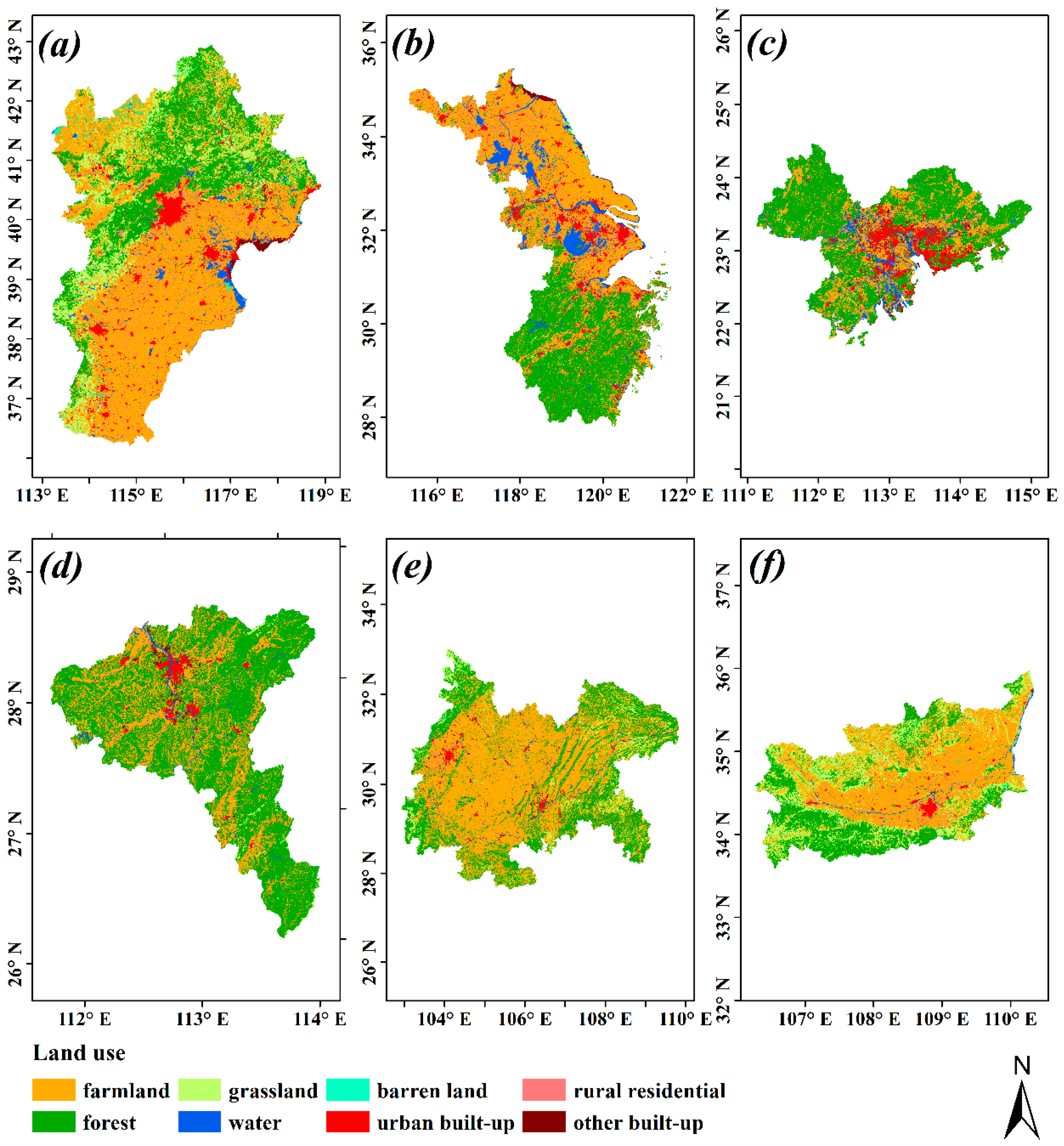
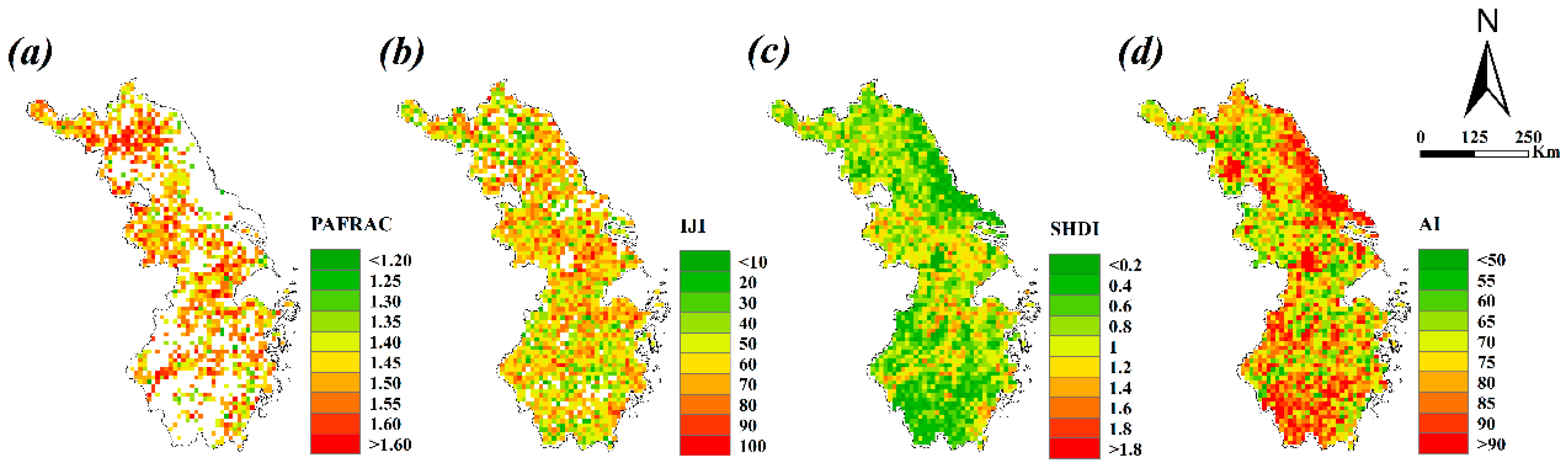
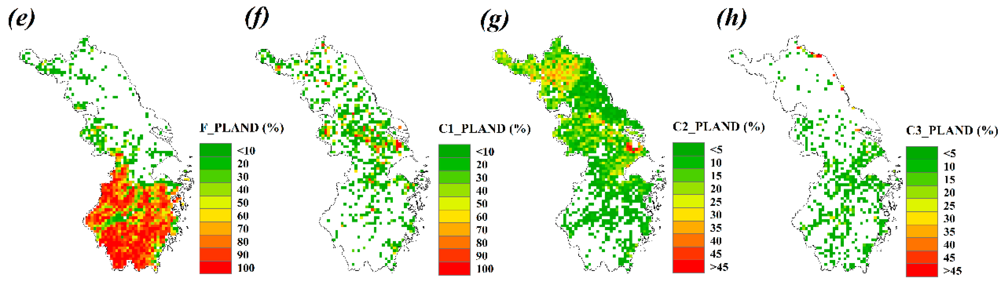
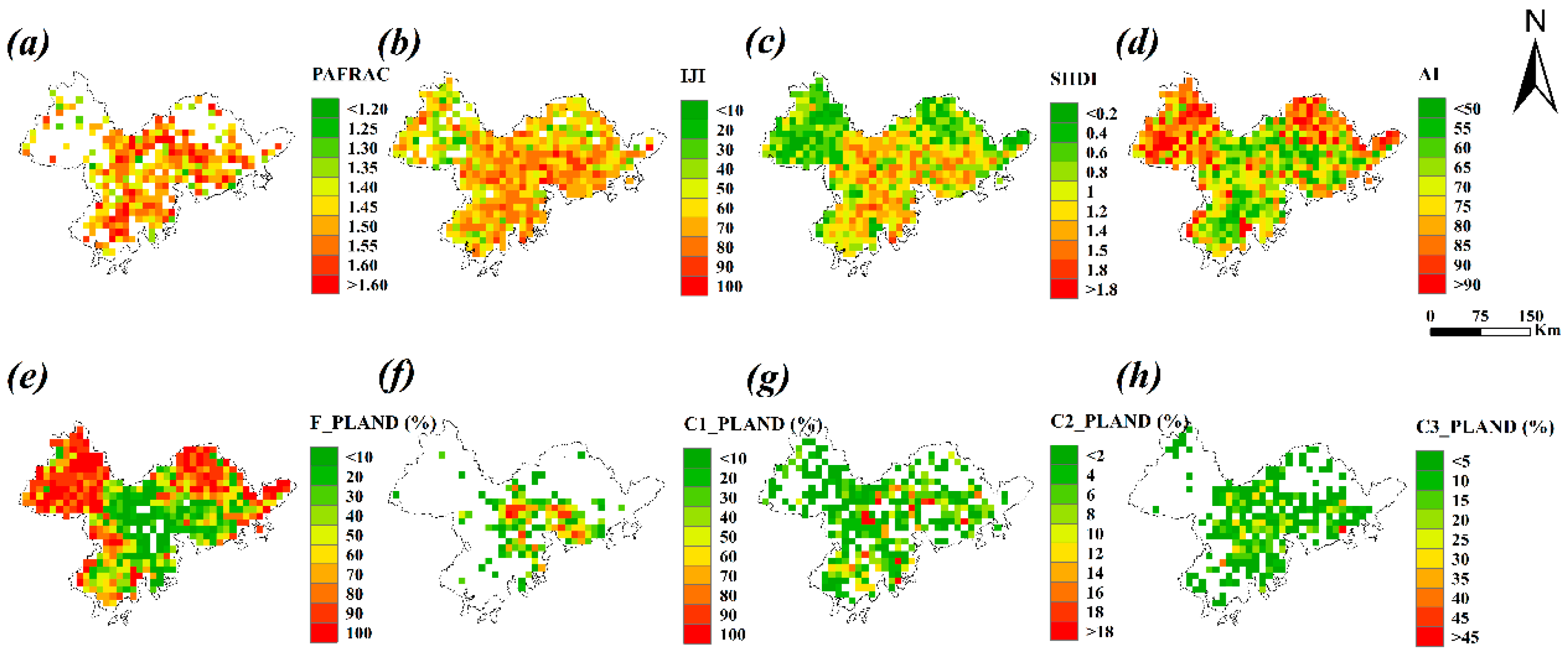
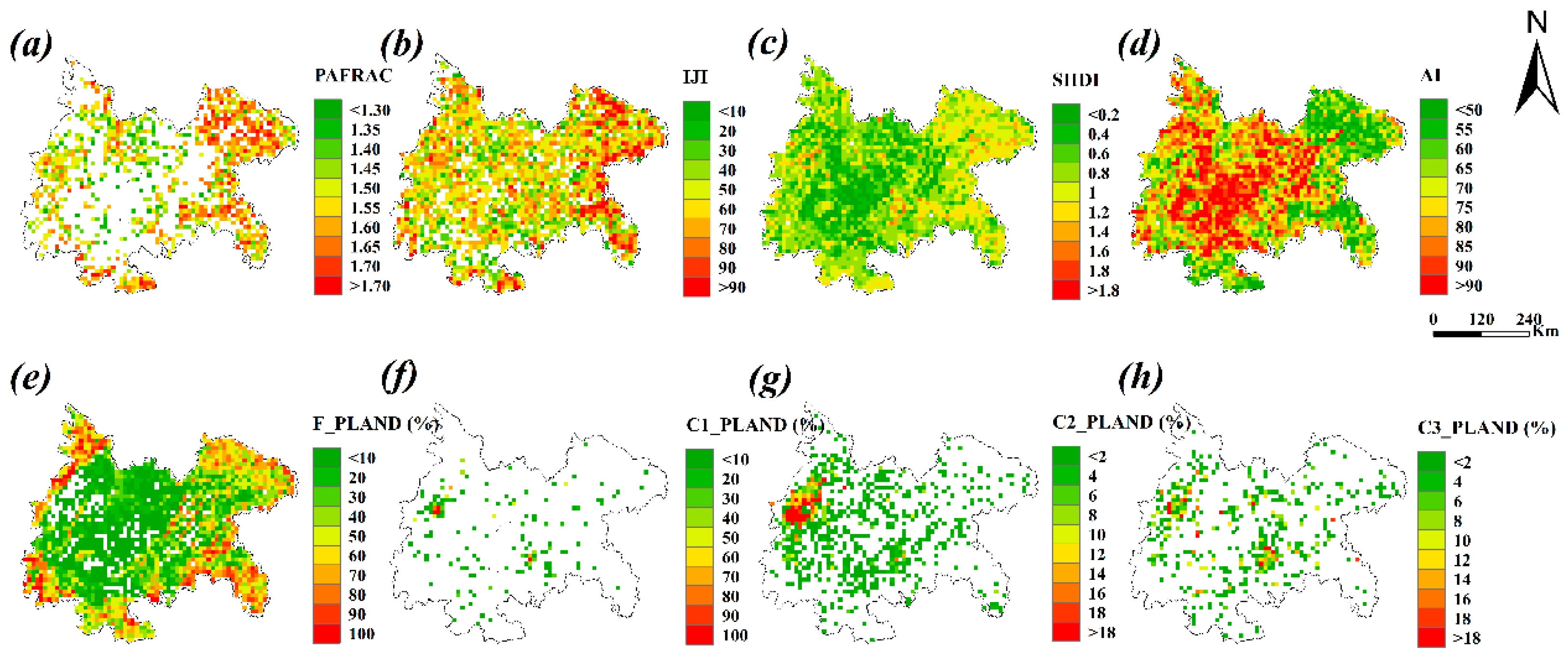
3.1. Land Use and Landscape Patterns

Figure 2 shows the spatial pattern of land use over the six urban agglomerations. Generally, farmland and forest dominate the types, which cover more than 60% of the area of the regions. The built-up areas are located in the center of all the urban agglomerations, which covers less than 10% of the total area. In the Jing-Jin-Ji region, farmland is mainly in the southeast, while forest is in the northwest. In the Yangtze River Delta, land use presents significant centralization, represented by farmland in the north and forests in the south. Land use in the Pearl River Delta is much more heterogeneous, characterized by the built-up covers large area (8.01%) near to the sea and the forest and farmland are around the city area. The condition of Chang-Zhu-Tan is similar to that of the Pearl River Delta, with the significant mixture of farmland and forest. In the Chengdu-Chongqing and Guanzhong urban agglomerations, farmland is located in the center, with forest around it.

Correspondingly, the landscape patterns of the six urban agglomerations are shown in Figure 3, Figure 4, Figure 5, Figure 6, Figure 7 and Figure 8. The coverage indices are consistent with the land use pattern, while the conditions of landscape are more complex. In the Jing-Jin-Ji region, landscape is more heterogeneous in north than that in the south, represented by high values of PAFRAC, IJI, and SHDI in the north and high AI in the south. In the Yangtze River Delta, PAFRAC, IJI, and AI are relative high, indicating the centralization of land use. In the Pearl River Delta, the PAFRAC, IJI, and SHDI are high in the south, which is mainly attributed to the high urbanization near to the seaboard. It presents a triangular pattern in the Chang-Zhu-Tan urban agglomeration, caused by the high urbanization of Changsha, Zhuzhou, and Xiangtan. In the Chengdu-Chongqing region, the centralization of urbanization results in high values of PAFRAC and IJI around the basin, while AI is much higher in the central region. In the Guanzhong urban agglomeration, multiple centers of urbanization could be observed, leading to the heterogeneous pattern over the region. It can be seen that land use and landscape pattern are spatially variable, which would play significant effects on the local or regional geographic process.

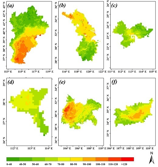
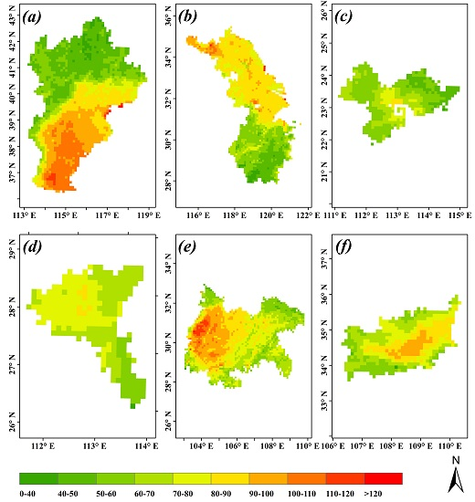
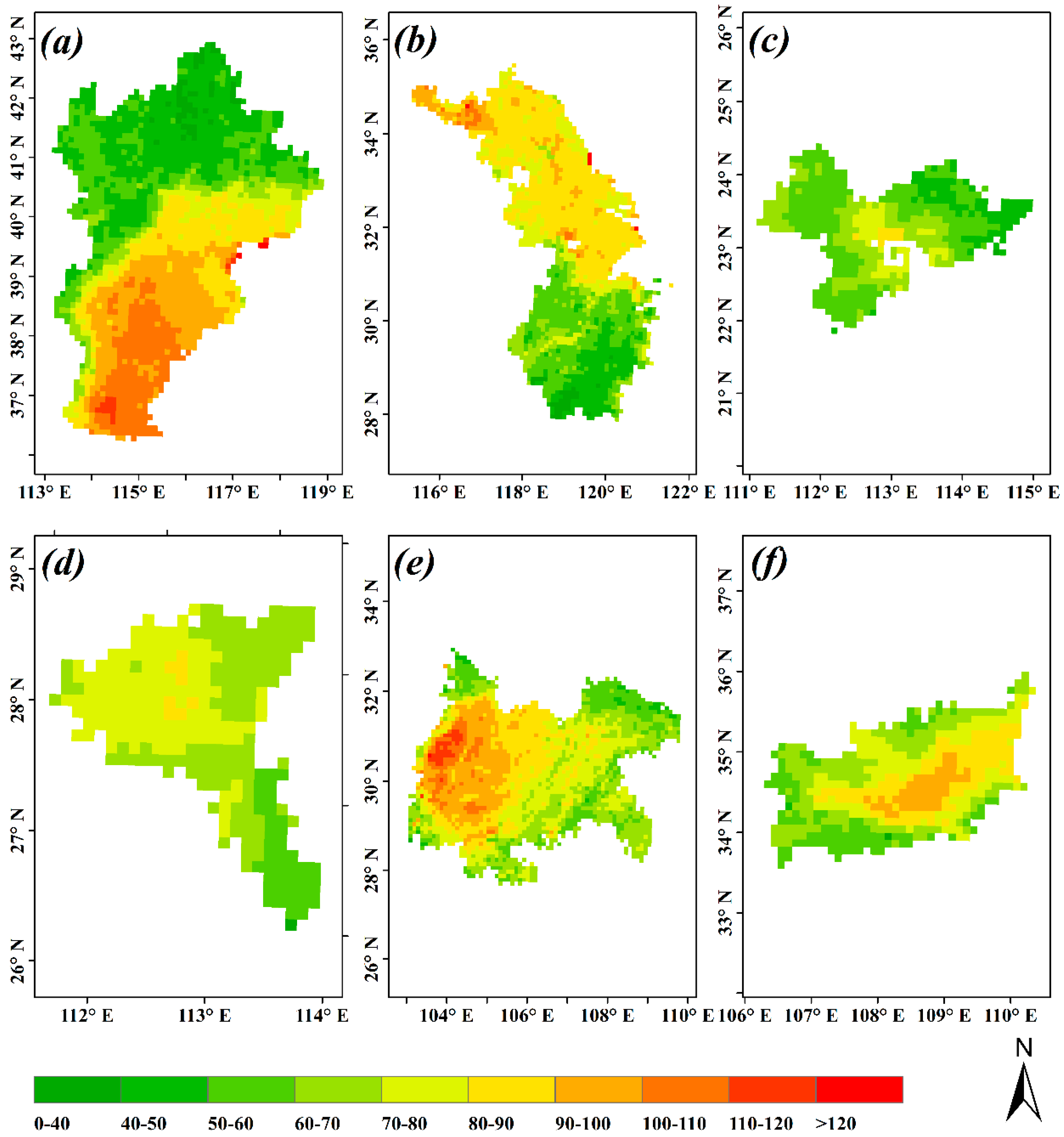
3.2. Variation of PM_2.5 Concentration

Based on the accurate TSAM-based results, we further investigate their correlations with the landscape. Under the condition of land use and landscape patterns, the PM_2.5 concentration present significant spatial variability. Averaged in situ data show that the concentration is highest in the Guanzhong (106.50 μg/m³) urban agglomeration, followed by the Jing-Jin-Ji (99.26 μg/m³), Chang-Zhu-Tan (82.46 μg/m³), Chengdu-Chongqing (71.68 μg/m³), and the Yangtze River Delta (68.76 μg/m³) regions, with the lowest concentration occurring in the Pearl River Delta (47.79 μg/m³). The TSAM-based data is used for further capturing the spatial pattern of PM_2.5 concentration at resolution of 10 km (Figure 9). Specifically, the concentration increases from north to south in the Jing-Jin-Ji region. In the Yangtze River Delta, the concentration is high in north, while it is low in the south. PM_2.5 is low in the Pearl River Delta, with the high concentration mainly located in the central of the region. With respect to the Chang-Zhu-Tan urban agglomeration, three hotspots of the high concentration could be identified in the urban area of the Changsha, Zhuzhou, and Xiangtan City. The concentration is high in Chengdu City in the Chengdu-Chongqing region, and decreases from the areas around the city. The condition of Guanzhong region is similar with that of Chengdu-Chongqing, with a high concentration in the center and lower around it.

3.3. Scale-Dependence of Landscape-PM_2.5 Correlation over Different Regions

3.3.1. In Situ Scale

The spatial pattern of land use exerts significant effect on the PM_2.5 concentration. We firstly evaluated the effect in the in situ site. For this aim, PM_2.5 concentration of all in situ sites and landscape indices in 500 m, 1000 m, 3000 m, 4000 m, and 5000 m buffers are adopted to evaluate the correlation.

Table 1. Correlation between landscape indices with PM_2.5 at different buffers (500, 1000, 3000, 4000, and 5000 m) of the in situ site in the six urban agglomerations.

Region (In-Situ Sites)	Buffer (m)	PAFRAC	IJI	SHDI	AI	F_PLAND	C1_PLAND	C2_PLAND	C3_PLAND
Jing-Jin-JI (80 sites)	500	−0.031	−0.158	−0.274 *	0.273 *	−0.166	0.224 *	0.017	0.010
	1000	−0.176	−0.251 *	−0.270 *	0.261 *	−0.18	0.244 *	−0.039	0.039
	3000	−0.336 **	−0.344 **	−0.351 **	0.0390 **	−0.215	0.297 **	−0.049	−0.111
	4000	−0.279 *	−0.167	−0.348 **	0.403 **	−0.267 *	0.320 **	−0.028	−0.095
	5000	−0.100	−0.098	−0.311 **	0.378 **	−0.308 **	0.328 **	−0.002	−0.080
Yangtze River Delta (162 sites)	500	−0.001	−0.053	−0.07	0.054	−0.114	0.115	−0.066	−0.017
	1000	−0.049	−0.074	−0.121	0.05	−0.160 *	0.126	−0.079	0.005
	3000	0.030	−0.019	−0.04	−0.023	−0.117	0.054	−0.021	−0.08
	4000	0.036	−0.037	−0.012	−0.04	−0.097	−0.001	0.073	−0.108
	5000	0.082	−0.071	−0.014	−0.05	−0.093	−0.032	0.118	−0.079
Pearl River Delta (55 sites)	500	−0.031	−0.011	−0.139	0.048	−0.147	0.160	−0.192	−0.029
	1000	−0.112	−0.206	−0.178	0.095	−0.290*	0.206	−0.211	−0.064
	3000	−0.220	−0.115	−0.219	0.229	−0.421 **	0.376 **	−0.223	−0.165
	4000	0.015	−0.093	−0.245	0.216	−0.462 **	0.423 **	−0.204	−0.212
	5000	−0.149	−0.300 *	−0.237	0.193	−0.479 **	0.434 **	−0.213	−0.25
Chang-Zhu-Tan (24 sites)	500	−0.112	0.087	0.044	0.088	−0.023	0.064	−0.245	0.006
	1000	0.038	0.144	0.067	0.029	−0.123	0.049	−0.212	0.015
	3000	−0.151	−0.026	−0.004	−0.105	−0.140	0.024	−0.120	−0.083
	4000	0.201	−0.131	−0.148	−0.027	−0.127	0.074	−0.167	−0.151
	5000	0.013	−0.124	−0.173	0.012	−0.182*	0.156*	−0.316	−0.225
Chengdu-Chongqing (53 sites)	500	−0.001	0.182	−0.026	0.122	−0.064	0.051	0.068	−0.164
	1000	0.178	0.178	0.208	−0.131	−0.053	−0.017	0.184	−0.137
	3000	0.091	0.180	0.202	−0.144	−0.272 *	0.006	0.129	−0.165
	4000	0.139	0.106	0.202	−0.252	−0.299 *	−0.025	0.027	−0.12
	5000	0.139	0.106	0.202	−0.252	−0.299 *	−0.025	0.027	−0.12
Guanzhong (33 sites)	500	0.050	0.076	0.145	−0.024	−0.061	−0.110	0.095	−0.115
	1000	0.098	0.034	0.259	−0.154	0.048	−0.170	0.034	−0.105
	3000	0.215	0.014	0.199	−0.216	−0.106	−0.230	0.075	0.015
	4000	0.093	−0.009	0.168	−0.193	−0.246 *	−0.218	0.080	−0.036
	5000	0.052	−0.141	0.122	−0.180	−0.262 *	−0.226 *	0.066	−0.08

** Represents significance at p < 0.01, while * means p < 0.05.

presents the correlation in the six urban agglomerations. Generally, landscape indices weakly correlate to the PM_2.5 concentration in most regions, suggesting that the landscape pattern has a relatively weak effect in these regions.

One exception can be found in the Jing-Jin-Ji region, which shows significant correlation between PM_2.5 concentration with landscape indices (significance at p < 0.05). Specifically, SHDI and F_PLAND show a negative correlation, while AI and C1_PLAND show a positive correlation. The correlation coefficient of SHDI and AI reach maximum at a distance of 4000 m to the in situ site, while those of F_PLAND and C1_PLAND reach the maximum at a distance of 5000 m. This suggests that the neighboring land use regulation has a potential influence on local PM_2.5 concentration. Correlation with F_PLAND and C1_PLAND are consistent with most previous studies, which revealed that forest could help to improve the air quality, while the urbanization could worsen the pollution [20,21,22,25,26,27]. The new finding of this study refers to the negative correlation of SHDI and positive correlation of AI in the Jing-Jin-Ji region. This suggests that a heterogeneous, rather than a homogeneous, landscape would be more effective for mitigating the local PM_2.5 concentration in th eJing-Jin-Ji region. Results provide a useful way for evaluating the existing urban pattern and guiding further planning to mitigate the PM_2.5 pollution in the Jing-Jin-Ji region. As the most serious pollution area in China, several land policies had been made and carried out to control the pollution (i.e., movement of the steel mills, greenbelt program around the ring, etc.), which helps to control the air pollution effectively [53,54,55]. There are dozens of parks in the in the Jing-Jin-Ji region [56]. Based on the results of this study, we also suggest enhancing the effects of parks with respect to numbers and locations.

Additionally, PM_2.5 concentration shows increasing correlation with the F_PLAND and C1_PLAND as the buffers increase (p < 0.01) in the Pearl River Delta. Urbanization in this region is characterized by a “bottom-up” mode, which worsens the air pollution [57]. By contrast, afforestation over the region would be an effective way to improve the air quality.

In the Chengdu-Chongqing urban agglomeration, only F_PLAND strongly correlates to the PM_2.5 concentration with a distance greater than 3000 m. Previous studies held the view that the meteorological factors determine the dispersion of PM_2.5 [58]. The results of this study show that forest could also pose an unavoidable effect on the pollution, particularly at a large scale. Therefore, more forest should be planted to improve the air quality.

Based on the results above, it can be concluded that the landscape pattern weakly correlates to in situ PM_2.5 concentration, while land use coverage has certain effects in some regions. Generally, the coverage of built-up areas and forest present relatively strong correlation. Therefore, afforestation over the region should be taken into consideration for controlling the local air pollution.

3.3.2. Regional Scale

In addition to the in situ site, we also investigate the correlation between landscape pattern and regional PM_2.5 concentration. Firstly, the landscape indices in each pixel (10 km) of TSAM-based PM_2.5 concentration is calculated. Then the values of the indices and PM_2.5 concentration from all the pixels are used to calculated the correlation coefficients over the selected regions (

Table 2. Correlation between the landscape with PM_2.5 at 10 km resolution of six urban agglomerations.

Region (Pixels)	PAFRAC	IJI	SHDI	AI	F_PLAND	C1_PLAND	C2_PLAND	C3_PLAND
Jing-Jin-Ji (2024 pixels)	−0.174 **	−0.335 **	−0.262 **	0.220 **	−0.642 **	0.188 **	0.613 **	0.132 **
Yangtze River Delta (2068 pixels)	0.218 **	0.068 **	0.205 **	−0.081 **	−0.807 **	0.235 **	0.555 **	0.031
Pearl River Delta (546 pixels)	0.413 **	0.413 **	0.442 **	0.044	−0.386 **	0.486 **	0.204 **	0.295 **
Chang-Zhu-Tan (291 pixels)	0.347 **	0.217 **	0.466 **	−0.05	−0.283 **	0.328 **	0.190 **	0.323 **
Chengdu-Chongqing (2253 pixels)	−0.065 **	0.026	−0.175 **	0.376 **	−0.567 **	0.160 **	0.412 **	0.197 **
Guanzhong (538 pixels)	0.228 **	0.111 *	0.145 **	0.419 **	−0.530 **	0.227 **	0.700 **	0.216 **

** Represents significance at p < 0.01, while * means p < 0.05.

). Results show that the indices almost strongly correlate to the concentration at the regional scale (significance at p < 0.01). This indicates that though landscape pattern present relative weak correlation to local PM_2.5 pollution (shown in Section 3.3.1), they would have a non-negligible effect on regional averaged concentration. Generally, F_PLAND shows the most significant correlation, followed by C2_PLAND and C1_PLAND, and IJI shows the weakest correlation. This indicates that the areas of land use would also have strong effects on the regional PM_2.5 concentration.

Another notable phenomenon is the sign of correlation in different regions. As expected, forest helps to mitigate air pollution, resulting in a negative correlation of F_PLAND. The urban and rural built-up areas worsen the pollution, leading to significantly positive correlations of C1_PLAND, C2_PLAND, and C3_PLAND. The conditions of other indices are more complex. Specifically, PAFRAC, SHDI, and IJI positively correlate to the concentration in most regions, except for the Jing-Jin-Ji and Chengdu-Chongqing regions. This means that the heterogeneous land use trends tend to worsen the total PM_2.5 pollution in most regions. The main reason might be the “bottom-up” urbanization in the Yangtze River Delta, the Pearl River Delta, the Chang-Zhu-Tan, and the Guanzhong regions. The heterogeneous urbanization results numerous pollution sources, which emits massive PM_2.5 [59,60]. In Jing-Jin-Ji and Chengdu-Chongqing regions, however, the urbanization is characterized by few highly-developed metropolitans, resulting in relatively centralized pollution sources [61,62]. Under this condition, the heterogeneous landscape might be helpful for the PM_2.5 dispersion over the regions [26,27,63]. The AI also positively correlates to the PM_2.5 concentration in most regions, except for the Yangtze River Delta and Chang-Zhu-Tan urban agglomerations. As shown in Figure 2 and Figure 4, several hotspots of the concentration could be identified in the two regions, which strongly correlate to the spatial pattern of land use. Therefore, the aggregation of the urbanization would reduce the emission sources, which would further help to control the air pollution of the total region.

3.3.3. Comparison of the Correlations at In Situ and Regional Scales

Correlations in Table 1 and Table 2 reveal significant differences at in situ and regional scales. To investigate the scale effect, this study then evaluates the correlation with aid of the selected PM_2.5 concentration and landscape indices from pixels where in situ sites located in (

Table 3. Correlation between landscape with TSAM-based PM_2.5 at the pixels with in situ sites.

Region (Pixels)	PAFRAC	IJI	SHDI	AI	F_PLAND	C1_PLAND	C2_PLAND	C3_PLAND
Jing-Jin-Ji	−0.124	0.206	−0.348 **	0.471 **	−0.438 **	0.485 **	0.284	0.433 **
Yangtze River Delta	−0.189	−0.197 *	−0.391 **	0.332 **	−0.432 **	0.341 **	0.295 **	−0.196
Pearl River Delta	0.227	−0.166	−0.296 *	0.184	−0.549 **	0.503 **	−0.266	0.010
Chang-Zhu-Tan	−0.090	0.585 **	0.394	0.027	−0.765 **	0.079	0.219	0.172
Chengdu-Chongqing	−0.283	0.070	−0.322 *	0.317 *	−0.402 *	0.446 **	−0.129	−0.287 *
Guanzhong	−0.408 *	0.029	−0.239	0.290	−0.568 **	0.562 **	0.045	−0.352

** Represents significance at p < 0.01, while * means p < 0.05.

). It can be seen that correlations in the selected pixels are stronger than those at in situ sites, while are weaker than those at regional scale. This suggests that land use and landscape play more significant effects on PM_2.5 concentration with the increasing spatial scales. Signs of the correlation are more complex in the Table 1, Table 2 and Table 3. Specifically, the signs of the selected pixels (Table 3) are similar to those of in situ sites (Table 1) at regions of Jing-Jin-Ji, Yangtze River Delta, Pearl River Delta, while they are opposite in Chengdu-Chongqing and Guanzhong urban agglomerations. By contrast, the signs are consistent between the selected pixels (Table 3) and the whole region (Table 2) in the Chengdu-Chongqing urban agglomeration, which are opposite in the Yangtze River Delta. As shown in Figure 3, Figure 4, Figure 5, Figure 6, Figure 7 and Figure 8, the Yangtze River Delta is characterized by “bottom-up” urbanization, while the Chengdu-Chongqing urban agglomeration is centralized urbanization. Under the former condition, correlations of in situ sites would be self-similar with those of the region. With respect to the centralized urbanization, the landscape is quite different at local and regional scales, leading to various correlations across different scales. The results above confirm that region-dependence, combined with the scale effect, strongly affect the correlation between landscape and PM_2.5 concentration.

4. Discussion

As described above, the landscape pattern presents a complex correlation to PM_2.5 concentration. Clarification of the correlation helps to capture the physical mechanism of the PM_2.5 concentration pattern, but it also helps to guide the urban planning and air pollution controlling.

The various correlations might be caused by the types of PM_2.5 and corresponding emission sources in different regions. In the Jing-Jin-Ji region, the PM_2.5 concentration is dominated by the quick secondary transformation of primary gaseous pollutants to secondary aerosols [64]. Fossil fuel combustion and vehicle emissions produced abnormally high amount of nitric oxide (NOx), resulting quick secondary transformation of coal-burning sulphur dioxide (SO₂) to sulphate aerosols. Furthermore, heterogeneous reactions on the surface of fine particles also promote the transformation from gaseous pollutants to secondary aerosols. On the other hand, the geographical and meteorological conditions lead to very unfavorable dispersions for PM_2.5, which worsens the air pollution. Under this condition, the heterogeneous land use (i.e., forest, build-up, road, etc.) could not only increases the absorption sources over the region, but also decreases the emission in the hotspots and enhances the dispersion. That means it would be an effective way to remove the centralized pollution sources for improving the air quality. The successful case can be found in the 2008 Olympic Games in Beijing. The Central People’s Government of China moves a great many polluting enterprises (i.e., the Capital Iron and Steel Company) out of Beijing. Due to those efforts, the air pollutant emission reduces more than 50% than before [65]. Furthermore, afforestation in the Jing-Jin-Ji region (i.e., the Green Belt in Beijing) had been confirmed as an effective way for controlling the PM_2.5 pollution [66,67].

In the Yangtze River Delta, organic matter was the most abundant composition in PM_2.5 (20–25% of total mass), followed by the inorganic ions [68]. The concentrations of organic matter, nitrate-containing particles (nitrate) and sulfate-containing particles (sulfate) increased significantly during the haze events. Furthermore, the high carbon-containing particles concentration was strongly impacted by the pollutants transported from surrounding cities [69]. Therefore, the heterogeneous land use means more emission sources of pollution, which leads to the positive correlation with the PM_2.5 concentration. In other words, the centralization of industrial land would reduce the pollution emission sources, which helps to control the PM_2.5 pollution. Additionally, forests are mainly located in the Northern Yangtze River Delta. The large coverage of forest would eliminate the PM_2.5 concentration. The centralization of forest would also compensate the high PM_2.5 concentration originates from the centralization industrial. In conclusion, the intensive development of industrial and forest land would be effective for controlling the PM_2.5 pollution.

Transportation and mobile vehicles are the two major PM_2.5 sources in the Pearl River Delta, contributing 62% and 21% of the total figure in December, and 42% and 28% in April. Another important cause of high PM levels has been the transport of PM_2.5 between cities [70]. It can be seen that urbanization plays one of the controlling factors for air pollution in the Pearl River Delta, which shows the most significant correlation compared to other regions of this study. Urbanization in the Pearl River Delta is characterized by the “bottom-up” form, which leads to heterogeneous emission sources over the region. Therefore, the polluted factories would be centralized developed in one or two cities, rather than in all cities. Public transportation, instead of private cars, should be developed and encouraged to reduce the pollution emission. Furthermore, more trees should be planted around the road to adsorb the PM_2.5 pollution.

Coal combustion and vehicle emissions were two major sources of PM_2.5 in the Chang-Zhu-Tan region, which accounted for about 35% and nearly 26% of the concentration. In addition, industrial emission, biomass burning, and urban dust are also significant sources. Additionally, the neighboring cities (i.e., Yueyang and Pingxiang) also play a certain influence on the region’s PM_2.5 formation [71]. Under this condition, PM_2.5 concentration presents a significantly positive correlation to the heterogeneous landscape indices (PAFRAC, IJI, and SHDI). To improve the air quality, it firstly needs to monitor the coal combustion, pollution emission of key enterprises, vehicle exhaust, and road dust. Then, the centralization of urban development should be taken into consideration to reduce the pollution emission and PM_2.5 transportation.

The condition of Chengdu-Chongqing urban agglomeration, represented by the negative correlation between PM_2.5 concentration and heterogeneous landscape, is similar to that of Jing-Jin-Ji region. The agglomeration has two centralized metropolitan areas which emit mass amounts of air pollution. Specifically, secondary inorganic aerosols, coal combustion, other industrial pollution, soil dust, vehicular emission, and metallurgical industry are the main sources for the PM_2.5, accounting for 37.5%, 22.0%, 17.5%, 11.0%, 9.8%, and 2.2% of the total concentration [72]. Climate conditions, particularly of low wind speed and high relative humidity, also are the controlling factors for PM_2.5 concentration [73]. Under this condition, the centralization of urbanization means difficulty in the dispersion of the pollution sources, which worsens the air quality. Therefore, it is an effective way to develop satellite cities to improve the air quality. Furthermore, the project of afforestation (i.e., urban greening) should be carried out to enhance the ability of PM_2.5 absorption.

PM_2.5 concentration strongly correlates to urbanization in the Guanzhong urban agglomeration. Industries and residential activities dominated PM_2.5 by about 83%. Energy production (mainly coal combustion) is the predominant source of secondary nitrate, contributing 46%. Statistically, the contributions of energy, industries, transportation, residential activities, dust, and other factors to PM_2.5 total mass are 5%, 58%, 2%, 16%, 4%, and 15% in Xi’an during the extremely polluted months [74]. Furthermore, regional pollution from biomass burning raised the concentrations of secondary ions while coal combustion was a strong influence during the winter episode [75]. Therefore, reduction of industry emission is most important issue for air pollution controlling. As shown in Table 2, the AI presents the most significant positive correlation. Therefore, it would be better to develop the suburban areas to avoid the centralized emission of PM_2.5.

Most previous studies revealed that climate dominates atmospheric dispersion conditions, which strongly affects PM_2.5 concentration [10,11,12,13,14,15]. The results of this study indicate that the interaction of climate enhances the complexity of correlation between PM_2.5 concentration and the landscape. In low atmospheric dispersion conditions (i.e., low wind speed), PM_2.5 concentration is more likely positively correlates with centralization of landscape (i.e., the Jing-Jin-Ji region and Chengdu-Chongqing urban agglomeration). That means the aggregated landscape enhances the centralized emission of PM_2.5, which tends to worsen the air pollution because of the low atmosphere self-purification capacity [76,77]. By contrast, the climate conditions are characterized by high dispersion (i.e., the high wind speed) in the Yangtze River Delta, the Pearl River Delta, the Chang-Zhu-Tan and Guanzhong urban agglomerations. Under these conditions, heterogeneous land use (particular of the built-up area) means the multi pollution sources, which strongly enhances the pollution transportation over the whole regions. Therefore, more attention should be paid to the combined effect of climate and land use for urban planning.

5. Conclusions

In this study, we evaluated the correlation between PM_2.5 concentration with land use and landscape patterns over six urban agglomerations in China. The results showed that both land use and landscape indices weakly correlate to PM_2.5 concentration at the in situ scale, while the strongly correlate to the concentration at the regional scale. This demonstrates that land use and landscape would affect the PM_2.5 at a large scale. Generally, F_PLAND shows the most significant correlation, followed by C2_PLAND and C1_PLAND, and IJI shows the weakest correlation. This indicates that the areas of land use, rather than their aggregations, play strong effects to the PM_2.5 concentration. F_PLAND shows negative correlation to the concentration, while C1_PLAND, C2_PLAND, and C3_PLAND present positive. It demonstrates that forest also helps to mitigate the regional air pollution, while urban and rural built-up worsen the pollution. PAFRAC, SHDI, and IJI positively correlate to the concentration in most urban agglomerations, suggesting that the heterogeneous landscape tends to worsen the PM_2.5 pollution in most regions. That is because heterogeneous distribution of urban pollution sources emits massive PM_2.5 in the whole region. Therefore, more heterogeneous land use would result in more serious air pollution.

Results of this study are very useful for urban planning and air pollution controlling. The first, and possibly most effective way, is to plant more trees to absorb PM_2.5. Correlation of the landscape pattern is strongly affected by climate condition, which should be taken into consideration. Generally, the heterogeneous pattern of urbanization is recommended in low atmospheric dispersion conditions (i.e., the Jing-Jin-Ji region and Chengdu-Chongqing urban agglomeration), which would reduce the centralized emission of PM_2.5. The climate conditions are characterized by high atmospheric dispersion in other regions of this study (the Yangtze River Delta, the Pearl River Delta, the Chang-Zhu-Tan, and Guanzhong urban agglomerations). Under this condition, the aggregated urban pattern means fewer emission sources, which would be diluted by atmospheric dispersion. Therefore, the homogeneous land use (particular of the built-up areas) would be more suitable for these regions. Other factors, i.e., rural and traffic emission, are the important issues in urban planning that warrant greater attention to be paid.

It could be concluded that the correlation between PM_2.5 concentration with landscape pattern varies with the spatial scales (site or regional) and the regions (six urban agglomerations). Therefore, more attention should be paid to the spatial variability of the correlation when modeling PM_2.5 concentration or in urban planning. Due to the collection of data, we investigated the correlation in one year. Longer time series data should be collected and used to evaluate the correlation for supporting the conclusion. Furthermore, though the adaptive land variables are used in the TSAM model, it unavoidably contains certain auto-correlation between the modeled PM_2.5 and landscape. The non-linear physical models, therefore, would be developed for improving the reliability and accuracy in our future studies.

References

1. Fann, N.; Lamson, A.D.; Anenberg, S.C.; Wesson, K.; Risley, D.; Hubbell, B.J. Estimating the National Public Health Burden Associated with Exposure to Ambient PM2.5 and Ozone. Risk Anal. 2012, 32, 81–95. [Google Scholar] [CrossRef] [PubMed]
2. Boldo, E.; Medina, S.; LeTertre, A.; Hurley, F.; Mücke, H.G.; Ballester, F.; Aguilera, I.; Eilstein, D. Apheis: Health Impact Assessment of Long-Term Exposure to PM2.5 in 23 European Cities. Eur. J. Epidemiol. 2006, 21, 449–458. [Google Scholar] [CrossRef] [PubMed]
3. Franklin, M.; Zeka, A.; Schwartz, J. Association between PM2.5 and All-Cause and Specific-Cause Mortality in 27 Us Communities. J. Exp. Sci. Environ. Epidemiol. 2007, 17, 279–287. [Google Scholar] [CrossRef] [PubMed]
4. Zhang, Q.; Jiang, X.; Tong, D.; Davis, S.J.; Zhao, H.; Geng, G.; Feng, T.; Zheng, B.; Lu, Z.; Streets, D.G.; et al. Transboundary Health Impacts of Transported Global Air Pollution and International Trade. Nature 2017, 543, 705–709. [Google Scholar] [CrossRef] [PubMed]
5. Huang, R.J.; Zhang, Y.; Bozzetti, C.; Ho, K.F.; Cao, J.J.; Han, Y.; Daellenbach, K.R.; Slowik, J.G.; Platt, S.M.; Canonaco, F.; et al. High Secondary Aerosol Contribution to Particulate Pollution During Haze Events in China. Nature 2014, 514, 218–222. [Google Scholar] [CrossRef] [PubMed] [Green Version]
6. Zhang, Y.L.; Fang, C. Fine Particulate Matter (PM2.5) in China at a City Level. Sci. Rep. 2015, 5, 14884. [Google Scholar] [CrossRef] [PubMed]
7. Wang, J.; Jia, X.; Rohit, M.; Jonathan, E.P.; Wang, S.; Christian, H.; Gan, C.M.; Wong, D.C.; Hao, J. Historical Trends in PM2.5-Related Premature Mortality During 1990–2010 across the Northern Hemisphere. Environ. Health Perspect. 2017, 125, 400–408. [Google Scholar] [CrossRef] [PubMed]
8. Liu, Y.; Li, Y.; Chen, C. Pollution: Build on Success in China. Nature 2015, 517, 145. [Google Scholar] [CrossRef] [PubMed]
9. Vayenas, D.V.; Takahama, S.; Davidson, C.I.; Pandis, S.N. Simulation of the Thermodynamics and Removal Processes in the Sulfate-Ammonia-Nitric Acid System during Winter: Implications for PM2.5 Control Strategies. J. Geophys. Res. Atmos. 2005, 110, D07S14. [Google Scholar] [CrossRef]
10. Cai, W.; Li, K.; Liao, H.; Wang, H.; Wu, L. Weather Conditions Conducive to Beijing Severe Haze More Frequent under Climate Change. Nat. Clim. Chang. 2017. [Google Scholar] [CrossRef]
11. Glavas, S.D.; Nikolakis, P.; Ambatzoglou, D.; Mihalopoulos, N. Factors Affecting the Seasonal Variation of Mass and Ionic Composition of PM2.5 at a Central Mediterranean Coastal Site. Atmos. Environ. 2008, 42, 5365–5373. [Google Scholar] [CrossRef]
12. Yao, X.; Chan, C.K.; Fang, M.; Cadle, S.; Chan, T.; Mulawa, P.; He, K.; Ye, B. The Water-Soluble Ionic Composition of PM2.5 in Shanghai and Beijing, China. Atmos. Environ. 2002, 36, 4223–4234. [Google Scholar] [CrossRef]
13. Yu, L.; Wang, G.; Zhang, R.; Zhang, L.; Song, Y.; Wu, B.; Li, X.; An, K.; Chu, J. Characterization and Source Apportionment of PM2.5 in an Urban Environment in Beijing. Aerosol Air Qual. Res. 2013, 13, 574–583. [Google Scholar] [CrossRef]
14. Vecchi, R.; Marcazzan, G.; Valli, G.; Ceriani, M.; Antoniazzi, C. The Role of Atmospheric Dispersion in the Seasonal Variation of Pm1 and PM2.5 Concentration and Composition in the Urban Area of Milan (Italy). Atmos. Environ. 2004, 38, 4437–4446. [Google Scholar] [CrossRef]
15. Allen, R.J.; Landuyt, W.; Rumbold, S.T. An Increase in Aerosol Burden and Radiative Effects in a Warmer World. Nat. Clim. Chang. 2016, 6, 269–274. [Google Scholar] [CrossRef]
16. Dawson, J.P.; Adams, P.J.; Pandis, S.N. Sensitivity of PM2.5 to Climate in the Eastern Us: A Modeling Case Study. Atmos. Chem. Phys. 2007, 7, 4295–4309. [Google Scholar] [CrossRef]
17. Querol, X.; Alastuey, A.; Rodriguez, S.; Plana, F.; Mantilla, E.; Ruiz, C.R. Monitoring of Pm10 and PM2.5 around Primary Particulate Anthropogenic Emission Sources. Atmos. Environ. 2001, 35, 845–858. [Google Scholar] [CrossRef]
18. Dennis, A.; Fraser, M.; Anderson, S.; Allen, D. Air Pollutant Emissions Associated with Forest, Grassland, and Agricultural Burning in Texas. Atmos. Environ. 2002, 36, 3779–3792. [Google Scholar] [CrossRef]
19. Heald, C.L.; Geddes, J.A. The Impact of Historical Land Use Change from 1850 to 2000 on Secondary Particulate Matter and Ozone. Atmos. Chem. Phys. 2016, 16, 14997–15010. [Google Scholar] [CrossRef]
20. Cheng, N.; Zhang, D.; Li, Y.; Fan, M. Residential Emissions in Beijing: About 400 × 104 T. In Proceedings of the National Academy of Sciences of the United States of America; National Academy of Sciences: Washington, DC, USA, 2016; Volume 113, pp. E5778–E5779. [Google Scholar]
21. Bozlaker, A.; Spada, N.J.; Fraser, M.P.; Chellam, S. Elemental Characterization of PM2.5 and Pm10 Emitted from Light Duty Vehicles in the Washburn Tunnel of Houston, Texas: Release of Rhodium, Palladium, and Platinum. Environ. Sci. Technol. 2014, 48, 54–62. [Google Scholar] [CrossRef] [PubMed]
22. Huang, Y.; Shen, H.; Chen, H.; Wang, R.; Zhang, Y.; Su, S.; Chen, Y.; Lin, N.; Zhuo, S.; Zhong, Q.; et al. Quantification of Global Primary Emissions of PM2.5, PM10, and Tsp from Combustion and Industrial Process Sources. Environ. Sci. Technol. 2014, 48, 13834–13843. [Google Scholar] [CrossRef] [PubMed]
23. Zhang, L.; Liu, Y.; Hao, L. Contributions of Open Crop Straw Burning Emissions to PM2.5 Concentrations in China. Environ. Res. Lett. 2016, 11, 014014. [Google Scholar] [CrossRef]
24. Xu, W.; Wu, Q.; Liu, X.; Tang, A.; Dore, A.J.; Heal, M.R. Characteristics of Ammonia, Acid Gases, and PM2.5 for Three Typical Land-Use Types in the North China Plain. Environ. Sci. Pollut. Res. 2016, 23, 1158–1172. [Google Scholar] [CrossRef] [PubMed]
25. Reddington, C.L.; Butt, E.W.; Ridley, D.A.; Artaxo, P.; Morgan, W.T.; Coe, H.; Spracklen, D.V. Air Quality and Human Health Improvements from Reductions in Deforestation-Related Fire in Brazil. Nat. Geosci. 2015, 8, 768–771. [Google Scholar] [CrossRef]
26. Matsuda, K.; Fujimura, Y.; Hayashi, K.; Takahashi, A.; Nakaya, K. Deposition Velocity of PM2.5 Sulfate in the Summer above a Deciduous Forest in Central Japan. Atmos. Environ. 2010, 44, 4582–4587. [Google Scholar] [CrossRef]
27. Dzierżanowski, K.; Popek, R.; Gawrońska, H.; Sæb, A.; Gawroński, S.W. Deposition of Particulate Matter of Different Size Fractions on Leaf Surfaces and in Waxes of Urban Forest Species. Int. J. Phytoremediat. 2011, 13, 1037–1046. [Google Scholar] [CrossRef] [PubMed]
28. Gehrig, R.; Buchmann, B. Characterising Seasonal Variations and Spatial Distribution of Ambient PM10 and PM2.5 Concentrations Based on Long-Term Swiss Monitoring Data. Atmos. Environ. 2003, 37, 2571–2580. [Google Scholar] [CrossRef]
29. Hueglin, C.; Gehrig, R.; Baltensperger, U.; Gysel, M.; Monn, C.; Vonmont, H. Chemical Characterisation of PM2.5, PM10 and Coarse Particles at Urban, near-City and Rural Sites in Switzerland. Atmos. Environ. 2005, 39, 637–651. [Google Scholar] [CrossRef]
30. Xu, G.; Jiao, L.; Zhang, B.; Zhao, S.; Yuan, M.; Gu, Y.; Liu, J.; Tang, X. Spatial and Temporal Variability of the PM2.5/PM10 Ratio in Wuhan, Central China. Aerosol Air Qual. Res. 2017, 17, 741–751. [Google Scholar] [CrossRef]
31. Wang, Y.; Zacharias, J. Landscape Modification for Ambient Environmental Improvement in Central Business Districts—A Case from Beijing. Urban For. Urban Green. 2015, 14, 8–18. [Google Scholar] [CrossRef]
32. Matzka, J.; Maher, B.A. Magnetic Biomonitoring of Roadside Tree Leaves: Identification of Spatial and Temporal Variations in Vehicle-Derived Particulates. Atmos. Environ. 1999, 33, 4565–4569. [Google Scholar] [CrossRef]
33. Pielke, R.A.; Avissar, R. Influence of Landscape Structure on Local and Regional Climate. Landsc. Ecol. 1990, 4, 133–155. [Google Scholar] [CrossRef]
34. Baró, F.; Chaparro, L.; Gómez-Baggethun, E.; Langemeyer, J.; Nowak, D.J.; Terradas, J. Contribution of Ecosystem Services to Air Quality and Climate Change Mitigation Policies: The Case of Urban Forests in Barcelona, Spain. AMBIO 2014, 43, 466–479. [Google Scholar] [CrossRef] [PubMed]
35. McCarty, J.; Kaza, N. Urban Form and Air Quality in the United States. Landsc. Urban Plann. 2015, 139, 168–179. [Google Scholar] [CrossRef]
36. Herold, M.; Goldstein, N.C.; Clarke, K.C. The Spatiotemporal Form of Urban Growth: Measurement, Analysis and Modeling. Remote Sens. Environ. 2003, 86, 286–302. [Google Scholar] [CrossRef]
37. Zhou, Q.; Li, B.; Kurban, A. Spatial Pattern Analysis of Land Cover Change Trajectories in Tarm Basin, Northwest China. Int. J. Remote Sens. 2008, 29, 5495–5509. [Google Scholar] [CrossRef]
38. McGarigal, K.; Cushman, S.A.; Neel, M.C.; Ene, E. Fragstats: Spatial Pattern Analysis Program for Categorical Maps. Available online: http://www.umass.edu/landeco/research/fragstats/fragstats.html (accessed on 1 September 2017).
39. Wu, J.; Xie, W.; Li, W.; Li, J. Effects of Urban Landscape Pattern on PM2.5 Pollution—A Beijing Case Study. PLoS ONE 2015, 10, e0142449. [Google Scholar] [CrossRef] [PubMed] [Green Version]
40. Weber, N.; Haase, D.; Franck, U. Assessing modelled outdoor traffic-induced noise and air pollution around urban structures using the concept of landscape metrics. Landsc. Urban Plann. 2014, 125, 105–116. [Google Scholar] [CrossRef]
41. Thomas, M.F. Landscape Sensitivity in Time and Space—An Introduction. CATENA 2001, 42, 83–98. [Google Scholar] [CrossRef]
42. Riveros-Iregui, D.A.; McGlynn, B.L. Landscape Structure Control on Soil Co2 Efflux Variability in Complex Terrain: Scaling from Point Observations to Watershed Scale Fluxes. J. Geophys. Res. Biogeosci. 2009, 114, G02010. [Google Scholar] [CrossRef]
43. Antrop, M. Landscape Change and the Urbanization Process in Europe. Landsc. Urban Plann. 2004, 67, 9–26. [Google Scholar] [CrossRef]
44. Geographical Information Monitoring Cloud Platform of China. Available online: http://www.dsac.cn/ (accessed on 20 June 2015).
45. China National Urban Air Quality Real-Time Publishing Platform Environmental Monitoring Center. Available online: http://113.108.142.147:20035/emcpublish/ (accessed on 13 March 2015).
46. LAADS Web. Available online: http://ladsweb.nascom.nasa.gov/ (accessed on 9 September 2016).
47. Benas, N.; Beloconi, A.; Chrysoulakis, N. Estimation of urban PM10 concentration, based on MODIS and MERIS/AATSR synergistic observations. Atmos. Environ. 2013, 79, 448–454. [Google Scholar] [CrossRef]
48. Song, W.; Jia, H.; Huang, J.; Zhang, Y. A satellite-based geographically weighted regression model for regional PM 2.5 estimation over the Pearl River Delta region in China. Remote Sens. Environ. 2014, 154, 1–7. [Google Scholar] [CrossRef]
49. Zou, B.; Wang, M.; Wan, N.; Wilson, J.G.; Fang, X.; Tang, Y. Spatial Modeling of PM2.5 Concentrations with a Multi-factoral Radial Basis Function Neural Network. Environ. Sci. Pollut. Res. 2015, 22, 10395–10404. [Google Scholar] [CrossRef] [PubMed]
50. Fang, X.; Zou, B.; Liu, X.; Sternberg, T.; Zhai, L. Satellite-Based Ground PM2.5 Estimation Using Timely Structure Adaptive Modeling. Remote Sens. Environ. 2016, 186, 152–163. [Google Scholar] [CrossRef]
51. Sun, P.; Xu, Y.; Yu, Z.; Liu, Q.; Xie, B.; Liu, J. Scenario Simulation and Landscape Pattern Dynamic Changes of Land Use in the Poverty Belt around Beijing and Tianjin: A Case Study of Zhangjiakou City, Hebei Province. J. Geogr. Sci. 2016, 26, 272–296. [Google Scholar] [CrossRef]
52. Buyantuyev, A.; Wu, J.; Gries, C. Multiscale analysis of the urbanization pattern of the Phoenix metropolitan landscape of USA: Time, space and thematic resolution. Landsc. Urban Plann. 2010, 94, 206–217. [Google Scholar] [CrossRef]
53. Wen, W.; Cheng, S.; Chen, X.; Wang, G.; Li, S.; Wang, X.; Liu, X. Impact of Emission Control on PM2.5 and the Chemical Composition Change in Beijing-Tianjin-Hebei During the Apec Summit 2014. Environ. Sci. Pollut. Res. 2014, 23, 4509–4521. [Google Scholar] [CrossRef] [PubMed]
54. Liu, J.; Mo, L.; Zhu, L.; Yang, Y.; Liu, J.; Qiu, D.; Zhang, Z.; Liu, J. Removal Efficiency of Particulate Matters at Different Underlying Surfaces in Beijing. Environ. Sci. Pollut. Res. 2016, 23, 408–417. [Google Scholar] [CrossRef] [PubMed]
55. Yang, J.; Zhou, J. The Failure and Success of Greenbelt Program in Beijing. Urban For. Urban Green. 2007, 6, 287–296. [Google Scholar] [CrossRef]
56. Li, W.; Ouyang, Z.; Meng, X.; Wang, X. Plant Species Composition in Relation to Green Cover Configuration and Function of Urban Parks in Beijing, China. Ecol. Res. 2006, 21, 221–237. [Google Scholar] [CrossRef]
57. Feng, H.; Liu, H.; Lv, Y. Scenario Prediction and Analysis of Urban Growth Using Sleuth Model. Pedosphere 2012, 22, 206–216. [Google Scholar] [CrossRef]
58. Li, Y.; Chen, Q.; Zhao, H.; Wang, L.; Tao, R. Variations in PM10, PM2.5 and PM1.0 in an Urban Area of the Sichuan Basin and Their Relation to Meteorological Factors. Atmosphere 2015, 6, 150–163. [Google Scholar] [CrossRef]
59. Wang, X.-R.; Hui, E.C.-M.; Choguill, C.; Jia, S.-H. The New Urbanization Policy in China: Which Way Forward? Habitat Int. 2015, 47, 279–284. [Google Scholar] [CrossRef]
60. Han, L.; Zhou, W.; Li, W. Increasing Impact of Urban Fine Particles (PM2.5) on Areas Surrounding Chinese Cities. Sci. Rep. 2015, 5, 12467. [Google Scholar] [CrossRef] [PubMed]
61. Haas, J.; Ban, B. Urban Growth and Environmental Impacts in Jing-Jin-Ji, the Yangtze, River Delta and the Pearl River Delta. Int. J. Appl. Earth Obs. Geoinform. 2014, 30, 42–55. [Google Scholar] [CrossRef]
62. Qu, W.; Zhao, S.; Sun, Y. Spatiotemporal Patterns of Urbanization over the Past Three Decades: A Comparison between Two Large Cities in Southwest China. Urban Ecosyst. 2014, 17, 723–739. [Google Scholar] [CrossRef]
63. Sun, F.; Yin, Z.; Lun, X.; Zhao, Y.; Li, R.; Shi, F.; Yu, X. Deposition Velocity of PM2.5 in the Winter and Spring above Deciduous and Coniferous Forests in Beijing, China. PLoS ONE 2014, 9, e97723. [Google Scholar] [CrossRef] [PubMed]
64. Wang, Y.S.; Yao, L.; Wang, L.; Liu, Z.; Ji, D.; Tang, G.; Zhang, J.; Sun, Y.; Hu, B.; Xin, J. Mechanism for the Formation of the January 2013 Heavy Haze Pollution Episode over Central, Eastern China. Sci. China Earth Sci. 2014, 57, 14–25. [Google Scholar] [CrossRef]
65. Wang, S.; Zhao, M.; Xing, J.; Wu, Y.; Zhou, Y.; Lei, Y.; He, K.; Fu, L.; Hao, J. Quantifying the air pollutants emission reduction during the 2008 Olympic Games in Beijing. Environ. Sci. Technol. 2010, 44, 2490–2496. [Google Scholar] [CrossRef] [PubMed]
66. Wang, G.; Bai, W.; Li, X.; Zhao, S. Research of greenbelt design technology on PM2.5 pollution reduction in Beijing. Chin. Landsc. Arch. 2014, 30, 71–76. (In Chinese) [Google Scholar]
67. Chen, J.; Yu, X.; Sun, F.; Lun, X.; Fu, Y.; Jia, G.; Zhang, Z.; Liu, X.; Mo, L.; Bi, H. The concentrations and reduction of airborne particulate matter (PM10, PM2.5, PM1) at shelterbelt site in Beijing. Atmosphere 2015, 6, 650–676. [Google Scholar] [CrossRef]
68. Shen, G.; Xue, M.; Yuan, S.; Zhang, J.; Zhao, Q.; Li, B.; Wu, H.; Ding, A. Chemical Compositions and Reconstructed Light Extinction Coefficients of Particulate Matter in a Mega-City in the Western Yangtze River Delta, China. Atmos. Environ. 2014, 83, 14–20. [Google Scholar] [CrossRef]
69. Wang, H.; An, J.; Shen, L.; Zhu, B.; Pan, C.; Liu, Z.; Liu, X.; Duan, Q.; Liu, X.; Wang, Y. Mechanism for the Formation and Microphysical Characteristics of Submicron Aerosol During Heavy Haze Pollution Episode in the Yangtze River Delta, China. Sci. Total Environ. 2014, 490, 501–508. [Google Scholar] [CrossRef] [PubMed]
70. Wu, D.; Fung, J.C.H.; Yao, T.; Lau, A.K.H. A Study of Control Policy in the Pearl River Delta Region by Using the Particulate Matter Source Apportionment Method. Atmos. Environ. 2013, 76, 147–161. [Google Scholar] [CrossRef]
71. Tang, X.; Chen, X.; Tian, Y. Chemical Composition and Source Apportionment of PM2.5—A Case Study from One Year Continuous Sampling in the Chang-Zhu-Tan Urban Agglomeration. Atmos. Pollut. Res. 2017. [Google Scholar] [CrossRef]
72. Chen, Y.; Xie, S.; Luo, B.; Zhai, C. Particulate Pollution in Urban Chongqing of Southwest China: Historical Trends of Variation, Chemical Characteristics and Source Apportionment. Sci. Total Environ. 2017, 584–585, 523–534. [Google Scholar] [CrossRef] [PubMed]
73. Wang, H.; Shi, G.; Tian, M.; Zhang, L.; Chen, Y.; Yang, F.; Cao, X. Aerosol Optical Properties and Chemical Composition Apportionment in Sichuan Basin, China. Sci. Total Environ. 2017, 577, 245–257. [Google Scholar] [CrossRef] [PubMed]
74. Wang, D.; Hu, J.; Xu, Y.; Lv, D.; Xie, X.; Kleeman, M.; Xing, J.; Zhang, H.; Ying, Q. Source Contributions to Primary and Secondary Inorganic Particulate Matter During a Severe Wintertime PM2.5 Pollution Episode in Xi’an, China. Atmos. Environ. 2014, 97, 182–194. [Google Scholar] [CrossRef]
75. Niu, X.; Cao, J.; Shen, Z.; Ho, S.S.H.; Tie, X.; Zhao, S.; Xu, H.; Zhang, T.; Huang, R. PM2.5 from the Guanzhong Plain: Chemical Composition and Implications for Emission Reductions. Atmos. Environ. 2016, 147, 458–469. [Google Scholar] [CrossRef]
76. Shi, K.; Liu, C.-Q. Self-Organized Criticality of Air Pollution. Atmos. Environ. 2009, 43, 3301–3304. [Google Scholar] [CrossRef]
77. Zhang, X.; Wu, L.; Zhang, R.; Deng, S.; Zhang, Y.; Wu, J.; Li, Y.; Lin, L.; Li, L.; Wang, Y.; et al. Evaluating the Relationships among Economic Growth, Energy Consumption, Air Emissions and Air Environmental Protection Investment in China. Renew. Sustain. Energy Rev. 2013, 18, 259–270. [Google Scholar] [CrossRef]
Figure 1. Study area.
Remotesensing 09 00918 g001
Figure 2. Spatial pattern of land use of (a) the Jing-Jin-Ji region; (b) the Yangtze River Delta; (c) the Pearl River Delta; (d) the Chang-Zhu-Tan; (e) the Chengdu-Chongqing; and (f) the Guanzhong urban agglomerations in 2013.
Remotesensing 09 00918 g002
Figure 3. Landscape patterns of (a) PAFRAC, (b) IJI; (c) SHDI; (d) AI; (e) F_PLAND; (f) C1_PLAND; (g) C2_PLAND; and (h) C3_PLAND in the Jing-Jin-Ji region.
Remotesensing 09 00918 g003
Figure 4. Landscape patterns of (a) PAFRAC; (b) IJI; (c) SHDI; (d) AI; (e) F_PLAND; (f) C1_PLAND; (g) C2_PLAND; and (h) C3_PLAND in the Yangtze River Delta.
Remotesensing 09 00918 g004aRemotesensing 09 00918 g004b
Figure 5. Landscape patterns of (a) PAFRAC; (b) IJI; (c) SHDI; (d) AI; (e) F_PLAND; (f) C1_PLAND; (g) C2_PLAND; and (h) C3_PLAND in the Pearl River Delta.
Remotesensing 09 00918 g005
Figure 6. Landscape patterns of (a) PAFRAC; (b) IJI; (c) SHDI; (d) AI; (e) F_PLAND; (f) C1_PLAND; (g) C2_PLAND; and (h) C3_PLAND in the Chang-Zhu-Tan urban agglomeration.
Remotesensing 09 00918 g006
Figure 7. Landscape patterns of (a) PAFRAC; (b) IJI; (c) SHDI; (d) AI; (e) F_PLAND; (f) C1_PLAND; (g) C2_PLAND; and (h) C3_PLAND in the Chengdu-Chongqing urban agglomeration.
Remotesensing 09 00918 g007
Figure 8. Landscape patterns of (a) PAFRAC; (b) IJI; (c) SHDI; (d) AI; (e) F_PLAND; (f) C1_PLAND; (g) C2_PLAND; and (h) C3_PLAND in the Guanzhong urban agglomeration.
Remotesensing 09 00918 g008
Figure 9. TSAM-based PM2.5 concentration (μg/m3) of (a) the Jing-Jin-Ji region; (b) the Yangtze River Delta; (c) the Pearl River Delta; (d) the Chang-Zhu-Tan; (e) the Chengdu-Chongqing; and (f) the Guanzhong urban agglomerations in 2013.
Remotesensing 09 00918 g009