Comparative Assessment of Two Vegetation Fractional Cover Estimating Methods and Their Impacts on Modeling Urban Latent Heat Flux Using Landsat Imagery

Abstract

Quantifying vegetation fractional cover (VFC) and assessing its role in heat fluxes modeling using medium resolution remotely sensed data has received less attention than it deserves in heterogeneous urban regions. This study examined two approaches (Normalized Difference Vegetation Index (NDVI)-derived and Multiple Endmember Spectral Mixture Analysis (MESMA)-derived methods) that are commonly used to map VFC based on Landsat imagery, in modeling surface heat fluxes in urban landscape. For this purpose, two different heat flux models, Two-source energy balance (TSEB) model and Pixel Component Arranging and Comparing Algorithm (PCACA) model, were adopted for model evaluation and analysis. A comparative analysis of the NDVI-derived and MESMA-derived VFCs showed that the latter achieved more accurate estimates in complex urban regions. When the two sources of VFCs were used as inputs to both TSEB and PCACA models, MESMA-derived urban VFC produced more accurate urban heat fluxes (Bowen ratio and latent heat flux) relative to NDVI-derived urban VFC. Moreover, our study demonstrated that Landsat imagery-retrieved VFC exhibited greater uncertainty in obtaining urban heat fluxes for the TSEB model than for the PCACA model.

1. Introduction

The urban heat island (UHI) is a phenomenon that leads to increased air or surface temperatures in urbanized areas compared to temperatures in surrounding rural areas. Recently, there has been an increasing trend in studies that quantify the urban heat island response to global environmental change, requiring the surface heat flux in energy balance models of cities. To enhance the understanding of energy and water exchanges across urban landscape environments, Grimmond et al. [1] and Grimmond et al. [2] compared 33 urban energy balance models, and the results showed that the models were most capable of modeling net all-wave radiation and least capable of modeling latent heat flux. However, most of them are numerical microclimate models and not compatible with the application of large-scale remote sensing data, considering the complex inputs of meteorological data and urban surface geometric characteristics.

To quantify global and regional energies, remote sensing data have been coupled with numerous physical models to enhance modeling accuracy [3,4]. Various physical models, such as the big-leaf theory models [5,6,7] and Surface Energy Balance System model [8,9], were developed to delineate surface energy components across urban landscape environments. Moreover, the two-source energy balance models, in which heat fluxes are calculated separately for each surface component (i.e., bare land and vegetation), were established to delineate the surface energy balance with relatively satisfactory accuracies [10,11,12,13,14,15]. In particular, Zhang et al. [16] and Zhang et al. [17] developed a more convenient Pixel Component Arranging and Comparing Algorithm (PCACA) model based on the two-layer model using a combination of land surface temperature (LST) and the vegetation fractional cover (VFC) space. Kuang et al. [18] achieved using PCACA model to quantify the effects of urban land-cover on surface heat flux regulation in Beijing. Recently, some improved temperature decomposition methods based on PCACA model were further proposed [19,20,21] to estimate regional heat fluxes.

VFC is a key input to remote sensing models of land surface energy balance in heterogeneous areas because the vegetation coverage influences energy exchange processes and heat fluxes of land surfaces. Considering surface energy balance models in urban landscape environments, sub-pixel heterogeneities in vegetation cover distributions can significantly impact model partitioning of available energy due to the nonlinearities inherent in land-atmosphere interactions. With respect to some remote sensing-based urban thermal studies [14,22], the influence of vegetation coverage on urban heat fluxes is generally evident in the determination of the associated heat flux component using linear or non-linear combinations of each fraction of urban land cover (mainly urban vegetation and non-vegetation). The effects of spatial heterogeneity resulting from mixed pixels of vegetation cover and other land covers over heterogeneous regions on the surface heat fluxes have been assessed by some studies using coarse resolution satellite imagery such as Moderate Resolution Imaging Spectrometer (MODIS) and Advanced Very High Resolution Radiometer (AVHRR). Gibson et al. [23] described the uncertainty related to VFC in the derivation of evapotranspiration using the Surface Energy Balance System model. Kustas and Norman [24] reported that heat energy balance modeling tended to be affected by landscape heterogeneity due to mixed pixel effects. However, satellite-based quantification of the impact of sub-pixel VFC on energy budgets at the urban scale using medium resolution imagery (i.e., Landsat) has received less attention than it deserves, particularly concerning different energy flux models.

Remote sensing provides a useful data source for quantifying VFC over large areas; however, many remote sensing data are not fine enough to retrieve VFC with very satisfactory results over regional landscapes [25]. Based on the resolutions of most operational satellite sensors such as Landsat and ASTER, spatial resolution limitations are evident in the context of characterizing VFC because complex urban landscape environments generally exhibit a mix of urban vegetation cover and impervious surfaces. To retrieve urban vegetation fractional coverage, the dimidiate pixel model has been performed with the image bands (or band math), such as the Normalized Difference Vegetation Index (NDVI) [26,27,28] and variations [29,30]. NDVI-derived method was extensively used to determine the VFC factor in urban heat flux assessments over regional areas [18,31,32,33]. However, satellite image-based vegetation indices were found to have low correlations with the VFC in heterogeneous landscapes such as dry lands or urban areas due to the sensitivity of vegetation to surface environmental conditions [34,35]. Spectral Mixture Analysis (SMA) is a sub-pixel classification technique, in which the spectrum collected by a sensor is assumed to be a linear or nonlinear combination of the spectra of components within the studied pixel level [36]. Linear SMA was efficient in estimating the percentage of ground cover, such as vegetation cover and impervious surfaces [37,38,39,40]. While these two methods (NDVI-derived and SMA-derived) were applied to urban environments to obtain VFC, very few studies have attempted to quantitatively evaluate their relative accuracies and associated roles in estimating urban heat fluxes [18,41].

Considering VFC is a key input parameter in the energy balance model and the effects of remote sensing VFC on the urban heat flux estimation have not been fully assessed, this research evaluated how the application of two different VFC retrieval models (NDVI-derived method and Multiple Endmember Spectral Mixture Analysis (MESMA)-derived method) affected the accuracies of the model estimates of surface heat fluxes in a heterogeneous urban environment. For this purpose, two urban heat fluxes models that used MESMA-derived and NDVI-derived VFC as inputs, the TSEB and PCACA models, were implemented across the urban landscape of Beijing, China. Moreover, inter-comparable studies of how the two different remote sensing-based urban heat flux models (TSEB and PCACA) with different physical basis depend on VFC were also conducted in our research. Thus, the Bowen ratio and latent heat fluxes were calculated based on four methods: (1) TSEB combined with NDVI-derived VFC; (2) TSEB combined with MESMA-derived VFC; (3) PCACA combined with NDVI-derived VFC; and (4) PCACA combined with MESMA-derived VFC.

2. Study Area and Data

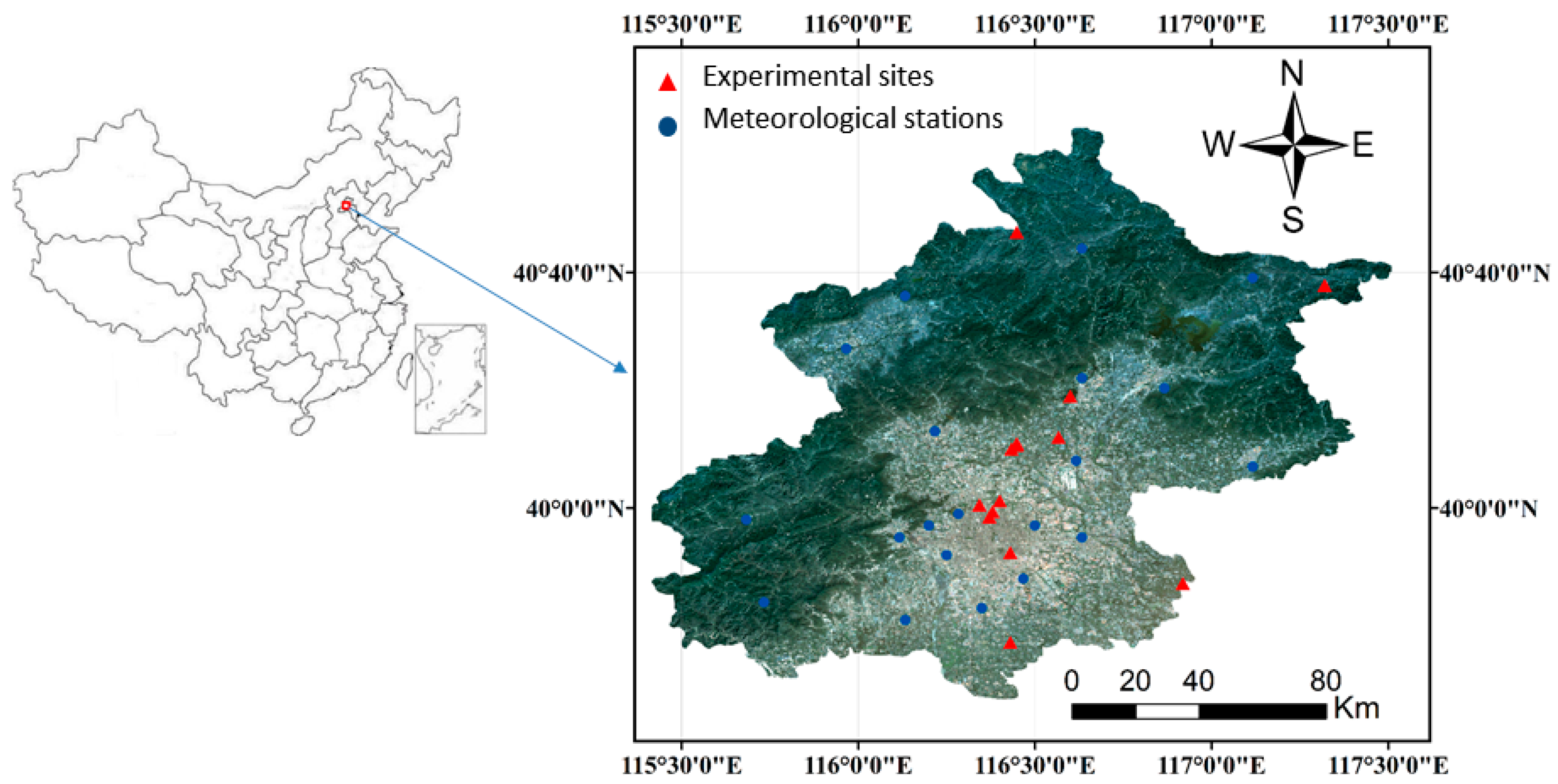
2.1. Study Area

Beijing (located at 39°28′N–41°05′N and 115°25′E–117°30′E) is the capital city of China (Figure 1) and selected for our research. This city exhibits high northwestern and low southeastern terrain and is surrounded by mountainous areas to the west and plains to the east and south. Beijing has experienced significant urban sprawl in recent decades. Quantification of urban thermal environments in Beijing is of great significance for sustainable urban development and residential comfort. By quantifying and comparing remote sensing-based energy balance models over Beijing, we can better understand the key surface factors that drive inter-model discrepancies.

2.2. Datasets

2.2.1. Remote Sensing Data

To quantify the urban heat fluxes, one cloud-free Landsat 5 TM image (22 September 2009) of Beijing was used. In addition, a QUICKBIRD image that covered the Beijing region was collected on 1 October 2009 and employed as a reference dataset for the identification of field data. To retrieve the atmospheric profile for estimating Landsat LST, we collected TERRA/MODIS remote sensing images (MOD021KM and MOD03, obtained online at http://daac.gsfc.nasa.gov/data/dataset/MODIS/), which have the same acquisition date as the Landsat TM imagery.

One Landsat scene available from 22 September 2009 may be insufficient, therefore ten Landsat TM/ETM images collected on 17 April 2001, 12 April 2002, 6 July 2004, 6 May 2005, 22 May 2005, 27 March 2008, 14 May 2008, 2 April 2010, 5 June 2010 and 21 June 2010 over Beijing area were used to supplement the comparative analysis.

2.2.2. Ground Data

To validate the remote sensing-retrieved heat fluxes, eddy flux measurements of the latent heat flux (LE), sensible heat flux (H) and Bowen ratio (H/LE) were obtained from the work of [18]. In their study, LE and H recorded at five sites were used, as shown in

Table 1. Descriptions of ground observation sites and field observations collected at Landsat passing.

ID	Sites	Latitude/Longitude	Land-Cover Types	Validation Purposes	LANDSAT Date
B1	Kexue Nanli	39.99	Built-up areas	ET/LST	22 September 2009
		116.38
B2	Olympic Forest Park	40.02	Urban park	ET/LST	22 September 2009
		116.4
B3	Mi Yun	40.63	Orchard	ET/LST	22 September 2009
		117.32
B4	Da Xing	39.62	Cropland	ET/LST	22 September 2009
		116.43
B5	Xiang He	39.78	Cropland	ET/LST	22 September 2009
		116.95
B6	Ecological Research Center	40.02	Built-up areas	LST	22 September 2009
		116.34
B7	Institute of Atmospheric Physics	39.97	Built-up areas	LST	22 September 2009
		116.37
B8	Botanical Teaching Garden	39.87	Built-up areas	LST	22 September 2009
		116.43
BA1	Shun Yi	40.20	Winter wheat	ET/LST	17 April 2001
		116.56
BA2	Xiao Tang Shan	40.16	Bare soil	ET/LST	12 April 2002
		116.43
BA3	Xiao Tang Shan South-1	40.17	Maize	ET/LST	7 June 2004
		116.44
BA4	Xiao Tang Shan North-1	40.18	Grassland	ET/LST	7 June 2004
		116.44
BA5	Xiao Tang Shan South-2	40.17	Bare soil	ET/LST	5 June 2005, 22 May 2005
		116.44
BA6	Xiao Tang Shan North-2	40.18	Grassland	ET/LST	5 June 2005, 22 May 2005
		116.44
BA7	Mi Yun	40.63 117.32	Orchard, Maize	ET/LST	27 March 2008, 14 May 2008, 5 June 2010, 21 June 2010
BA8	Da Xing	39.62 116.43	Cropland	ET/LST	14 May 2008, 2 April 2010, 5 June 2010, 21 June 2010

. The observation instruments were installed approximately 20–30 m above the ground, with average values collected at half-hour intervals. Meteorological data from 20 meteorological stations in Beijing were collected based on [18].

In addition, eight field observations (BA1–BA8, in Table 1) collected in Beijing region during 2001 to 2010 were used for further accuracy comparison analysis. More detailed descriptions about the experiment sites can be found in [42,43].

To obtain the critical coefficients for the NDVI-derived VFC retrieval method and evaluate the precision of VFC images retrieved from Landsat TM, 150 sample plots were randomly selected in Beijing, and the corresponding reference VFC values were digitized using high-resolution QUICKBIRD imagery and Google Earth™ imagery. Specifically, reference fractions of urban vegetation abundance were obtained by manually digitizing 150 sample plots in the high-resolution imagery. Eight sites and field-measured VFC data from [18] were also used in this study. Among the 158 selected sites, 38 sites were used to retrieve the required coefficients for the NDVI-derived approach, and the other 120 sites were used to validate the Landsat TM VFC.

In addition, subsets of 10 and 23 sample plots located at the centers of pure water bodies and pure dry, bare lands (impervious surfaces and dry bare soil) were identified from the high-resolution QUICKBIRD and Google Earth™ images. Their corresponding Landsat TM LSTs were used to calibrate the input parameters of the PCACA model.

2.2.3. Image Pre-Processing

The collected Landsat images were first geo-referenced to the Universal Transverse Mercator (UTM) coordinate system using high-resolution Google Earth™ images. The RMSEs of the rectification were all less than one pixel for all the Landsat images. The atmospheric correction was applied to the visible and near infrared bands of Landsat imagery using the Fast Line-of-Sight Atmospheric Analysis of Spectral Hypercubes (FLAASH) module [44] in ENVI 4.8 software.

In this study, the land surface temperature (LST) was derived from the Landsat thermal infrared band, as described by Jiménez-Muñoz and Sobrino [45]. Land surface emissivity, which is necessary for retrieving LST, was obtained with NDVI thresholds method [46]. The accuracy of Landsat derived LST was assessed with the 26 field observations listed in Table 1. It is observed that a better agreement existed between the estimates and the measurements, and the Landsat estimation achieved an RMSE of 1.57 K and a MAE of 0.68 K.

Surface land cover maps were generated using image classification of Landsat TM/ETM images. This study utilized a non-parametric supervised classification based on support vector machine classifier [47]. Six predominant land cover types (i.e., forest, crops/grassland, bare soil, lawn, impervious surfaces and water bodies) were identified. High-resolution data sources including QuickBird and Google Earth™ were used to assess the classification results. The statistical measures involving overall accuracy (OA) and Kappa statistic (KC) were calculated. All of the images achieved acceptable results with the OA higher than 85% and KC higher than 0.90, meaning that the resultant Landsat classifications are reliable for further analysis.

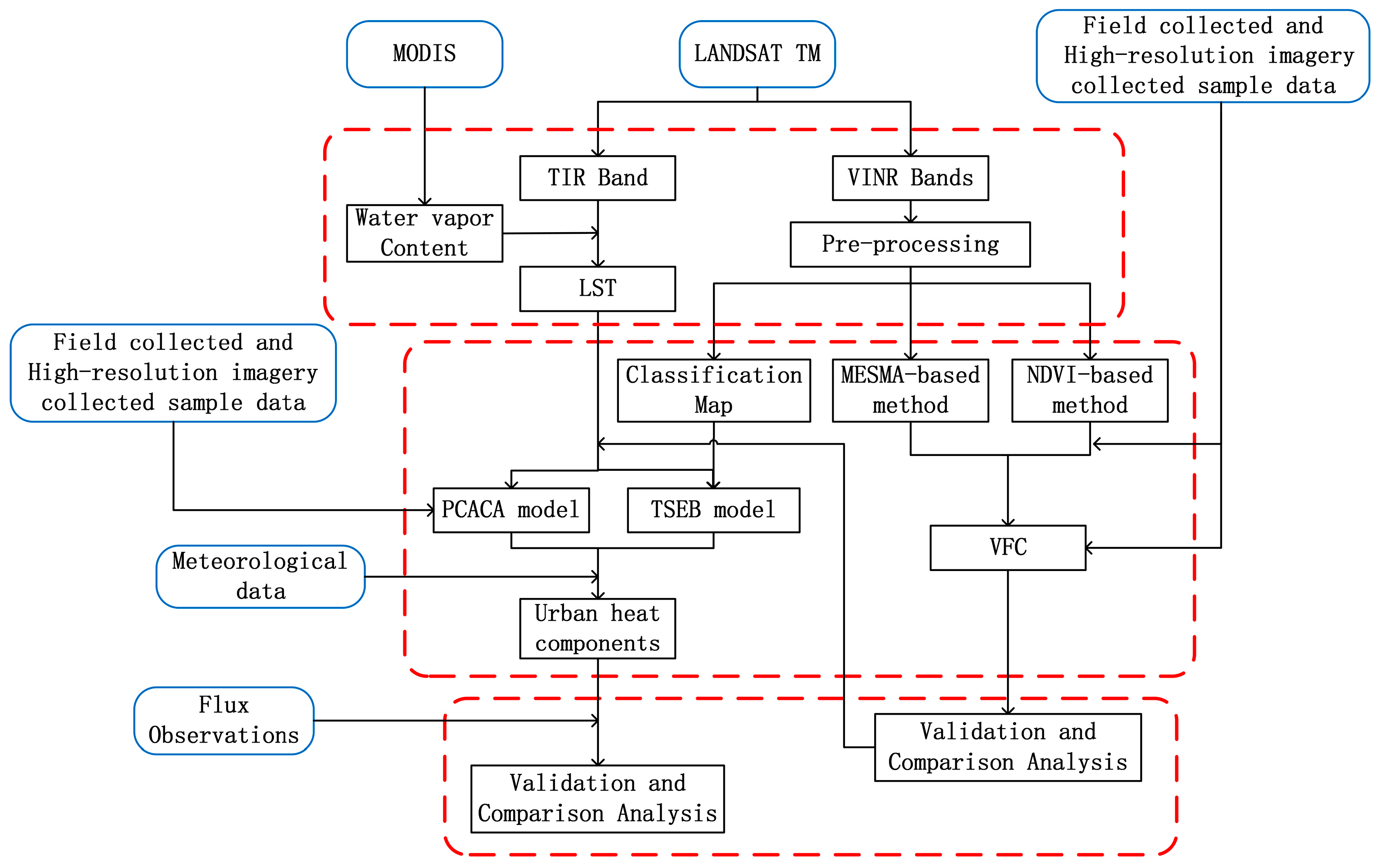
3. Method Description

The NDVI-derived model and MESMA-derived model were employed to predict surface VFC. Two models (TSEB model and PCACA model) with different physical basis were then used to investigate the urban heat flux. The overall flowchart is given in Figure 2.

3.1. Vegetation Coverage Retrieval

3.1.1. NDVI-Derived Method

The present study calculated the VFC with a simple and extensively used model, which obtains the VFC using a predefined function of the NDVI values. This model can be described as follows:

$$VFC={(\frac{NDVI-NDV{I}_s}{NDV{I}_v-NDV{I}_s})}^k$$

(1)

where $NDV{I}_v$ and $NDV{I}_s$ are the NDVI values of fully vegetated areas and bare land, respectively. $NDV{I}_v$ and $NDV{I}_s$ are required coefficients and generally depend on the specific research region. The coefficient k is a function associated with the vegetation distribution. k is set to 1 in this study, as suggested by [18,22,26,27].

In the retrieval of VFC by the NDVI-derived method, mean Landsat TM NDVI values at 23 selected bare land locations (8 bare soil and 15 impervious surfaces) were computed and considered as $NDV{I}_s$, and the value was set to 0.06. To estimate $NDV{I}_v$, Equation (1) was implemented to fit the VFC values collected from high-resolution data and their corresponding values of $NDVI-NDV{I}_s$ at 38 sample sites (introduced in Section 2.2.2). The fitted value of $NDV{I}_v-NDV{I}_s$ = 0.60, and $NDV{I}_v$ was set to 0.66. It should be mentioned that $NDV{I}_v$ across the Beijing region was somewhat low in present study mainly due to the complex surface characteristics. Similar results were also found in some prior studies that focused on the VFC derivations over urban regions or desert regions, such as $NDV{I}_v$ = 0.60, in Beijing, China [18]; $NDV{I}_v$ = 0.63, in north China [48]; and $NDV{I}_v$ = 0.61, in central New Mexico, USA [27]. Therefore, the value of $NDV{I}_v$ reported by our study was reasonable and acceptable.

3.1.2. MESMA-Derived Method

Multiple endmember spectral mixture analysis (MESMA) [49,50,51] is an improved and widely used algorithm based on the linear SMA. Unlike other simple linear spectral mixture analyses, MESMA can unmix each pixel with different combinations of represented endmembers. The main advantage of MESMA is that it is able to overcome the limitation of using the fixed types and numbers of endmembers to model all pixels. MESMA mainly involves three steps. In the first step, the representative endmembers containing unique spectral reflectance were selected. Three major representative categories of urban land cover types (vegetation, soil and impervious surfaces with high-albedo and low-albedo) were identified based on VIS theory [52]. Water and wetland area were not considered and masked out in the pre-process procession due to the non-availability of MESMA model for water regions. Then, with these collected endmembers, a linear spectral unmixing analysis with full abundance constraints (Equations (2) and (3)) was performed to estimate fractional land covers in an iterative manner.

$$R={\displaystyle \sum _{k=1}^n{f}_k{R}_k}$$

(2)

$${\displaystyle \sum _{k=1}^n{f}_k=1,}{f}_k\ge 0$$

(3)

where $k$ is the number of endmembers, $f_k$ is the fraction of endmember $k$, and $R_k$ is the reflectance of endmember $k$.

In the process of implementing MESMA, a series of simple linear spectral mixture analysis models were used to diversify the combinations of endmembers. For each pixel, one-, two-, and three-endmember combinations were used to determine the optimal candidate model. An optimal candidate model generates a realistic range of fractions (0–100%) and does not exceed an RMSE threshold (0.025). The corresponding estimated results of MESMA were combined into one image with several associated bands. Each band represents the areal fraction of each endmember of vegetation, bare soil and impervious surfaces. VFC can be obtained as the sum of all the abundance bands of vegetation.

This study established a spectra library consisting of 28 spectra. Specifically, some major candidate imagery endmembers were first identified using the Pixel purity index approach in combination with an N-dimensional visualizer. Then, the optimal representative endmembers were chosen from the diverse collected endmembers. The high-albedo and low-albedo impervious surface categories each included 6 distinct endmember spectra, and the vegetation (grassland/lawn and forest) and bare soil categories included 6/5 and 5 spectra, respectively. The reflective spectra of the collected endmembers are displayed in Figure 3. With the selected endmember spectra, MESMA was implemented to obtain VFC. In the process of MESMA, a large number of combination models were applied to unmix each pixel in a cyclical manner. The associated details of MESMA model parameterization are shown in

Table 2. Details of the MESMA model parameterization.

Data	Type of Combination	Number of Models	Total
Landsat TM	one-endmembers	28
	two-endmembers	313	2087
	three-endmembers	1746

.

3.2. Urban Heat Flux Retrieval

3.2.1. TSEB Model

An advanced two-source urban heat flux algorithm [14,15] is applied to delineate heterogeneous urban areas. This model can decompose the heat flux within a mixed pixel into sub-component heat fluxes of vegetation and non-vegetation.

For single observation angle satellite data, it is impractical to accurately separate the component surface temperatures of the vegetation and the impervious surface within the complex mixed pixels. Thus, the sensible heat flux $H$ is obtained using an alternative effective resistance approach:

$$H=\rho C_p\frac{T_s-T_a}{VFC\times R_{a\_veg}+(1-VFC)\times R_{a\_non-veg}+R_s}$$

(4)

where $\rho$ is the air density, $C_p$ is the specific heat of air at constant pressure, $T_s$ is the remote sensing surface temperature from Landsat imagery and $T_a$ is the atmospheric temperature. $R_{a\_veg}$ and $R_{a\_non-veg}$ are the aerodynamic resistance values of vegetated and non-vegetated areas, respectively, which are retrieved using the following equation:

$$R_a=\frac{\ln \left(\frac{Z_m-d}{Z_{0m}}\right)\times \ln \left(\frac{Z_h-d}{Z_{0h}}\right)}{k^{2}u}$$

(5)

where $Z_m$ is the height of wind measurements, $Z_h$ is the height of humidity measurements, $d$ is the zero-plane displacement height, $Z_{0m}$ is the roughness length governing momentum transfer, $Z_{0h}$ is the roughness length governing transfer of heat and vapor, $k$ is the von Karman’s constant and $u$ is the wind speed (m s⁻¹) at a given height based on meteorological data.

$R_s$ is the resistance to heat flow in the boundary layer immediately above the soil surface and can be computed using the following equation:

$$R_s=\frac{1}{a+b{u}_s}$$

(6)

where $a$ is the free convective velocity, $b$ is a coefficient that represents the typical soil surface roughness, and $u_s$ is the wind speed over the soil surface at a height of 0.05–0.2 m. As suggested by Kustas and Norman [53] and Weng, Hu, Quattrochi and Liu [14], $a$ and $b$ are set to 0.004 m/s and 0.012, respectively.

LE is given using the following equation:

$$LE=VFC\times L{E}_{veg}+(1-VFC)\times L{E}_{non-veg}$$

(7)

where $L{E}_{veg}$ and $L{E}_{non-veg}$ are the latent heat fluxes in vegetated and non-vegetated areas, respectively. These variables were computed as follows:

$$\begin{array}{l}L{E}_{veg}=\frac{\rho C_p}{\gamma }\times \frac{e^o-e_a}{R_{a\_veg}+r_{s\_veg}}\\ L{E}_{non-veg}=\frac{\rho C_p}{\gamma }\times \frac{e^o-e_a}{R_{a\_non-veg}+r_{s\_non-veg}}\end{array}$$

(8)

where $e_a$ is the atmospheric water vapor pressure in hPa, $e^o$ is the saturation vapor pressure in hPa and is calculated using Equations (9) and (10) [5,7]. $\gamma$ is the psychometric constant.

$$\begin{array}{l}{e}^o=1013.25\exp (13.3185t_R-1.9760t_R{}^2-0.6445t_R{}^3\\ -0.1299t_R{}^4)\end{array}$$

(9)

$$t_R=1.0-\frac{373.15}{T}$$

(10)

In Equations (9) and (10), $T$ is the atmospheric temperature in kelvin and $r_{s\_veg}$ and $r_{s\_non-veg}$ are the stomata resistance values in vegetated and non-vegetated areas, respectively. $r_{s\_veg}$ and $r_{s\_non-veg}$ were obtained using the simple approach reported by Kato and Yamaguchi [5].

By dividing sensible heat flux $H$ by latent heat flux $LE$, we can obtain the Bowen ratio.

$$\beta =\frac{H}{LE}$$

(11)

In the TSEB model, the required parameters involving roughness lengths, including d, $Z_{0m}$ and $Z_{0h}$, have important influences on the results. Typical values of d, $Z_{0m}$ and $Z_{0h}$ for specific surface land types are alternatively used in this study. The reference classifications of the surface types were obtained using the SVM method. Based on existing studies in the Beijing [54,55], the required parameters are listed in

Table 3. Parameters used for surface coverage types.

Land Cover	${\mathit{Z}}_{\mathbf{0}\mathit{m}}$ (m)	${\mathit{Z}}_{\mathbf{0}\mathit{m}}$/${\mathit{Z}}_{\mathbf{0}\mathit{h}}$	d (m)
Water	0.3 × 10−4	0.32	0
Bare soil	0.001	50	0
Crop field	0.12	100	0.02
Lawn	0.001	50	0.13
Forest	0.5–1.0	1000	4
Urban areas	1	1000	5

.

3.2.2. PCACA Model

The PCACA model uses a combination of LST versus VFC trapezoid method and a Bowen ratio energy balance method to partition surface temperature and surface net radiation of mixed pixels, subsequently estimating various heat components.

As a method that is based on the trapezoid approach, PCACA assumes that the LSTs of mixed pixels all exist within the space constructed by VFC and LST. In Figure 4, the wet edge of the trapezoid is related to surface conditions of maximum LE (or potential evapotranspiration). In contrast, the dry edge represents minimum LE (or zero evapotranspiration). Accordingly, if the endpoints of the two edges are selected and the associated positions are determined, we can fix the shape and structure of the trapezoid. Furthermore, the Bowen ratio and surface heat flux can be calculated.

In urban regions, $LS{T}_{sw}$ and $LS{T}_{sd}$ represent the endpoints of water bodies and dry, bare lands, respectively. $LS{T}_{vd}$ and $LS{T}_{vw}$ represent dry, full canopy green spaces and water-saturated soils, respectively. As described by previous studies [16,17,56], the Bowen ratio of each pixel can be retrieved through the linear interpolation between wet and dry edges of the trapezoid using the following equation:

$$\beta \approx {\left[\frac{LST-LS{T}_{\min }}{LS{T}_{\max }-LST}\right]}_{VFC}$$

(12)

where $LS{T}_{\min }$ and $LS{T}_{\max }$ are the intersections between VFC and the wet edge and dry edge, respectively. $LS{T}_{\min }$ and $LS{T}_{\max }$ in Figure 4 can be represented by the following equations:

$$\begin{array}{l}LS{T}_{\max }=k_{dry}\times VFC+LS{T}_{sd}\\ LS{T}_{\min }=k_{wet}\times VFC+LS{T}_{sw}\end{array}$$

(13)

where $k_{dry}$ and $k_{wet}$ are the slopes of the dry and wet edges. Substituting $LS{T}_{\min }$ and $LS{T}_{\max }$ in Equation (12) into Equation (13) yields the following expression.

$$\beta =\frac{-k_{wet}\times VFC-(LS{T}_{sw}-LST)}{k_{dry}\times VFC+(LS{T}_{sd}-LST)}$$

(14)

To determine appropriate $LS{T}_{\min }$ and $LS{T}_{\max }$ for the PCACA method, we must identify appropriate wet and dry edges in the complex urban regions using the Landsat-based VFC/LST spaces. Selecting accurate hot and cold endpoints is difficult because of the constraint information derived from one thermal band. In this study, we did not focus on the procedures used to identify extreme pixels. Following previous studies [16,17], $LS{T}_{sd}$ and $k_{dry}$ were retrieved using LST values from representative bare land in the study area, and $LS{T}_{sw}$ and $k_{wet}$ from the Landsat images were based on the LST values of several water districts in the study regions.

In the implementation of the PCACA model, 10 water bodies in Beijing were selected, and their mean Landsat TM LSTs were calculated. We considered the water surface temperature to be $LS{T}_{sw}=20.0\pm 0.5{}^{\mathrm{o}}\mathrm{C}.$ Average values of 23 Landsat TM LSTs of built-up, pavement and dry, bare soil regions in the study area were used to determine the dry surface temperature $LS{T}_{sd}=38.2\pm 0.9{}^{\mathrm{o}}\mathrm{C}$. When obtaining values of $LS{T}_{sw}$ and $LS{T}_{sd}$, $k_{dry}$ and $k_{wet}$ were estimated through fitting Equation (13) using a combination of VFC and LST. $k_{dry}$ and $k_{wet}$ were set to −4.76 and 0.51, respectively, in our study. With these calculated coefficients, the Bowen ratio was estimated from VFC and LST in each pixel using the following formula.

$$\beta =\frac{-0.51\times VFC-(20.0-LST)}{-4.76\times VFC+(38.2-LST)}$$

(15)

Then, based on Equations (1) and (12), LE can be obtained using Equation (16).

$$LE=\frac{R_n-G}{1+\beta }$$

(16)

In this study, $R_n$ and $G$ are estimated according to the work of [6,14].

4. Results

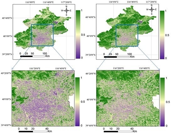
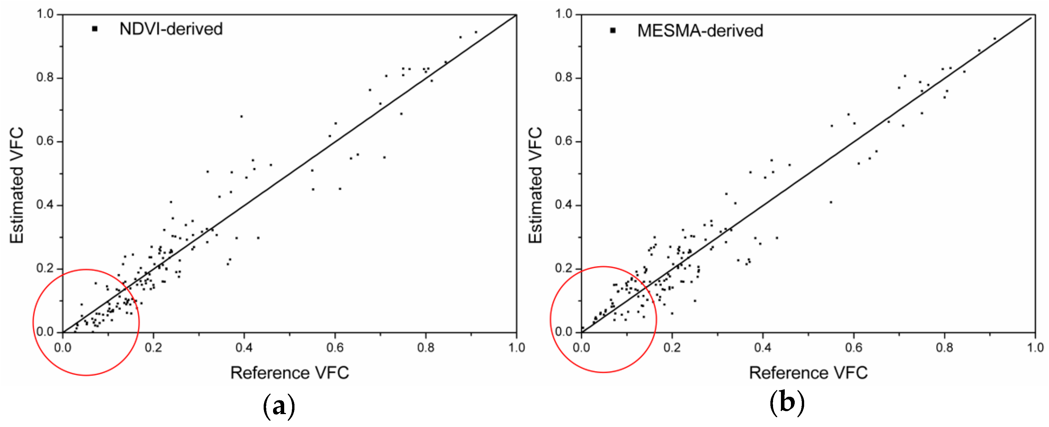
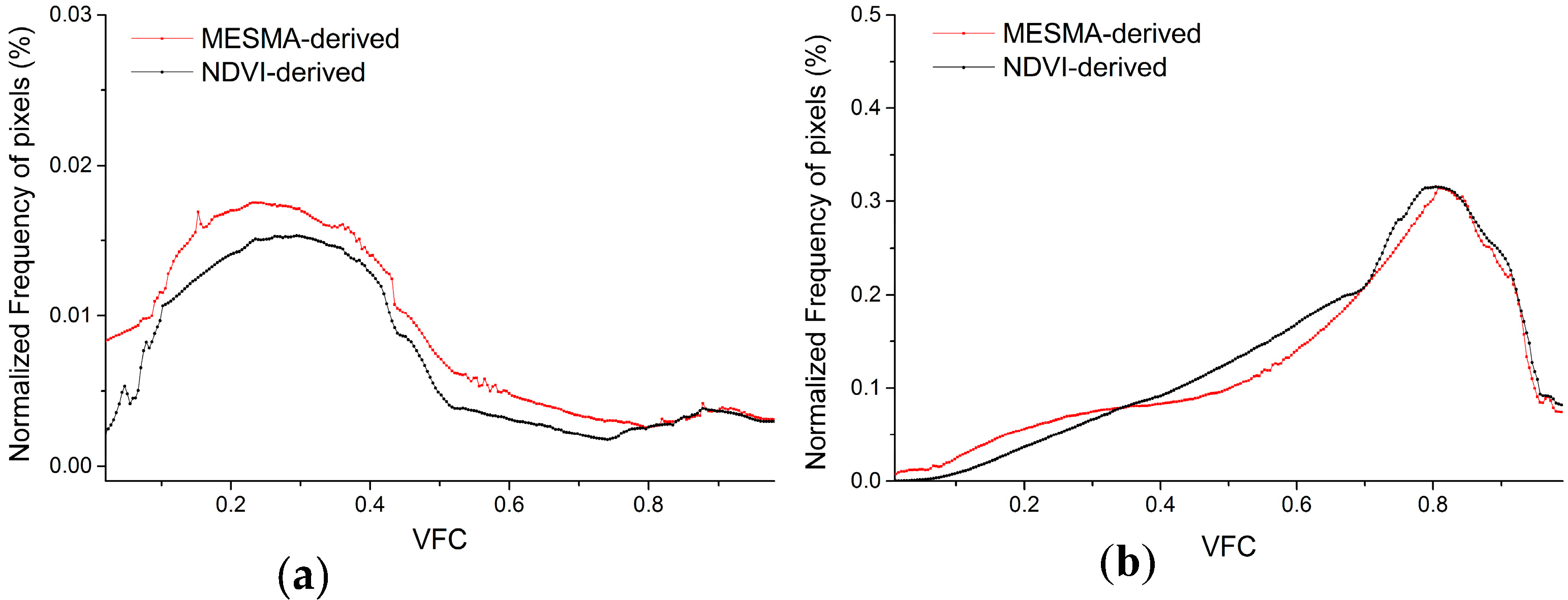
4.1. Performance of VFC Estimations

The resultant VFCs were validated using the independent dataset (N = 120) that is introduced in Section 2.2.2. The VFC maps derived from the two remote sensing methods are shown in Figure 5, and the scatter plots of estimated VFC versus reference VFC are given in Figure 6. Through checking the accuracy of NDVI-derived VFC, an adjusted R² of 0.86 was obtained. The regression analysis displayed an adjusted R² of 0.91 based on the results of the MESMA-derived method. For comprehensive analysis, urban landscape was subdivided into two categories: pixels were classified as less-developed areas when the VFC were larger than or equal to 30%, whereas those pixels of less than 30% were considered developed areas. The statistical results for the overall study area and two categories are illustrated in

Table 4. Comparisons of VFC estimation accuracy for NDVI-derived and MESMA-derived methods.

Error Assessment		NDVI-Derived (%)	MESMA-Derived (%)
RMSE	Overall	7.19	5.58
	Less developed areas	5.68	4.7
	Developed areas	9.65	8.35
MAE	Overall	5.82	4.79
	Less developed areas	5.32	3.91
	Developed areas	8.4	7.09

. The RMSE-based and MAE-based accuracies achieved using the MESMA-derived approach were 1.61% and 1.03% better, respectively, than those of the NDVI-based approach.

The resultant VFCs were approximately similar for the NDVI-derived and MESMA-derived methods in non-urban regions. Specific differences in the estimated VFCs obtained using these two methods were observed in urban regions. As shown in Figure 5, the spatial VFC patterns of trees and grasslands located in medium-high VFC areas (i.e., urban parks and residential areas) matched relatively well between the two methods. However, some small patches of grass/shrubs and trees located in low VFC areas, e.g., in the city center and the southern portions of built-up regions, were confused with impervious surfaces and resulted in obvious differences in estimated VFCs using the two methods. The better performance of the MESMA-derived method relative to that of the NDVI-derived method is also displayed by the red circles in scatter plots in Figure 6.

The performance of VFC retrieval was examined by comparing the frequency plots of estimated VFC values based on the NDVI-derived and MESMA-derived models. Figure 7 shows that the frequency profiles of the modeled VFC results are similar in non-urban regions, with a total bias of only 0.92. Conversely, the discrepancy between the NDVI-derived and MESMA-derived histograms in urban regions was relatively large, with a total bias of 3.12, indicating that the effectiveness of urban VFC retrieval varied between the two approaches. These deviations agree with the results of the conducted accuracy evaluations and scatter plots in Figure 6.

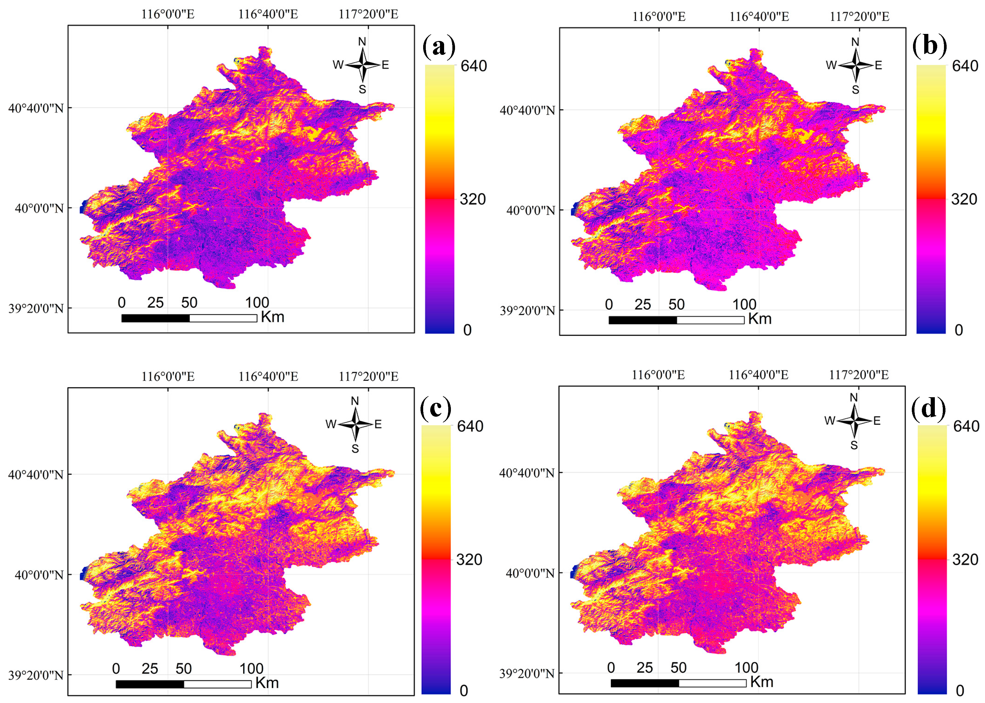
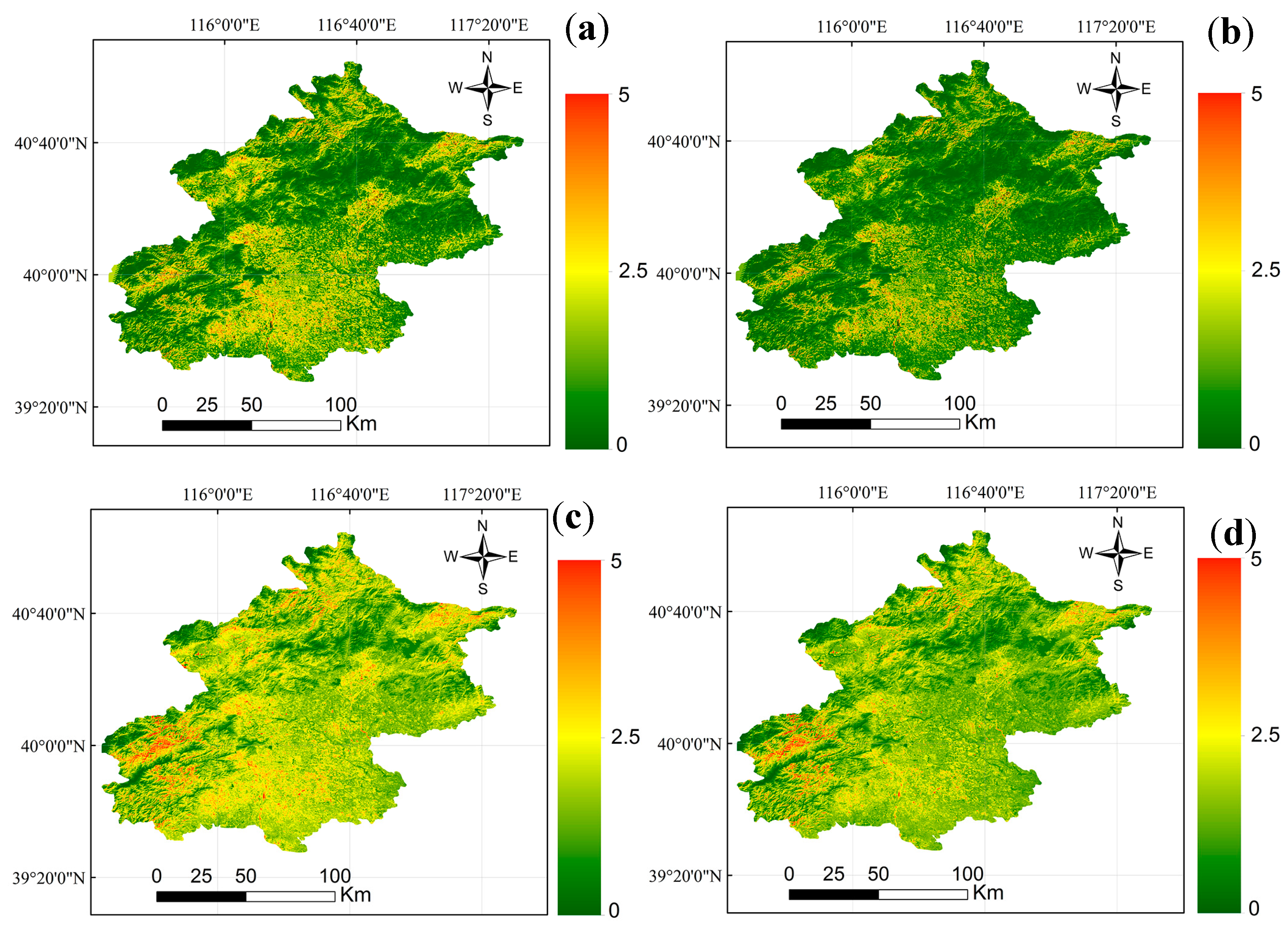
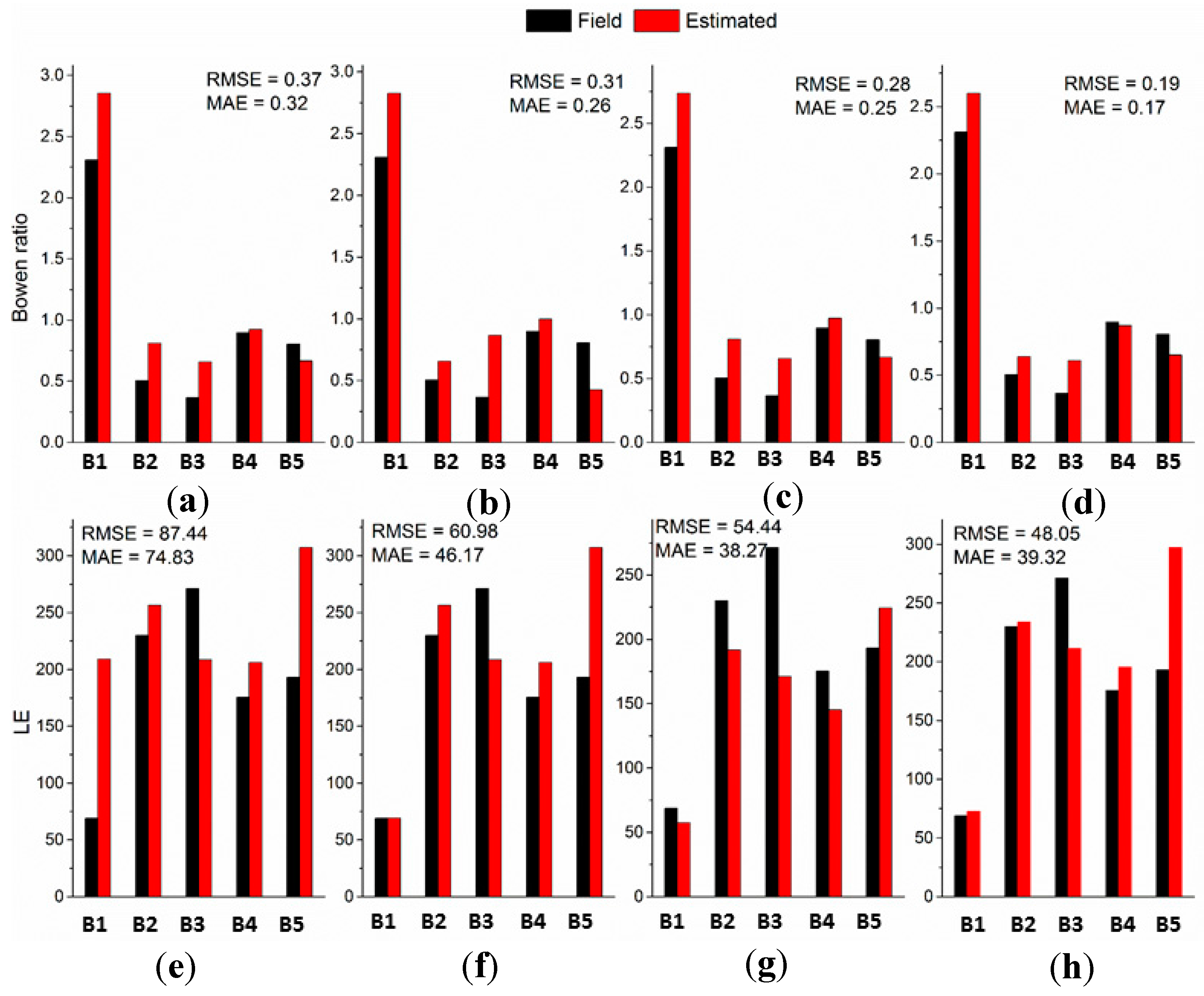
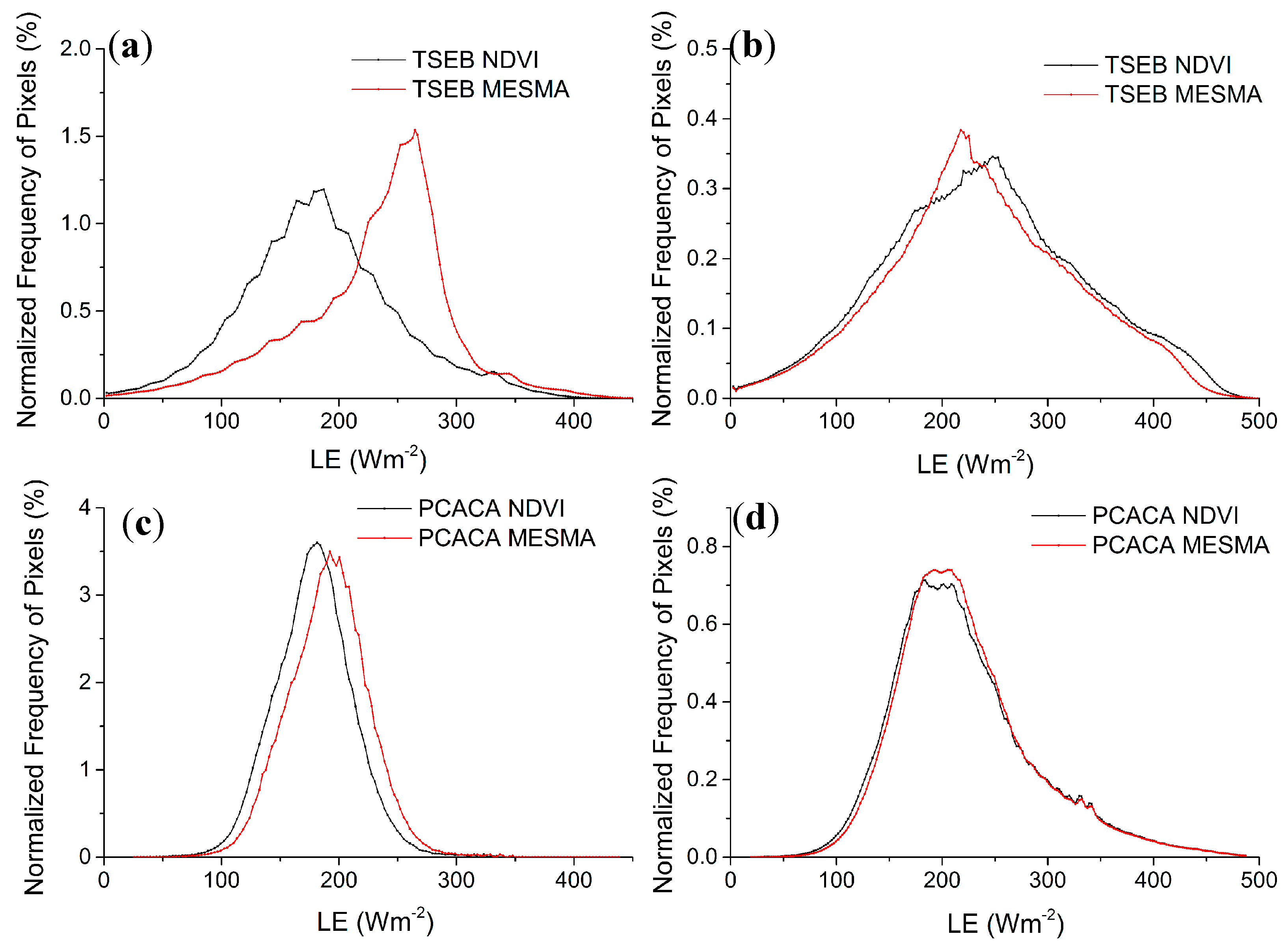
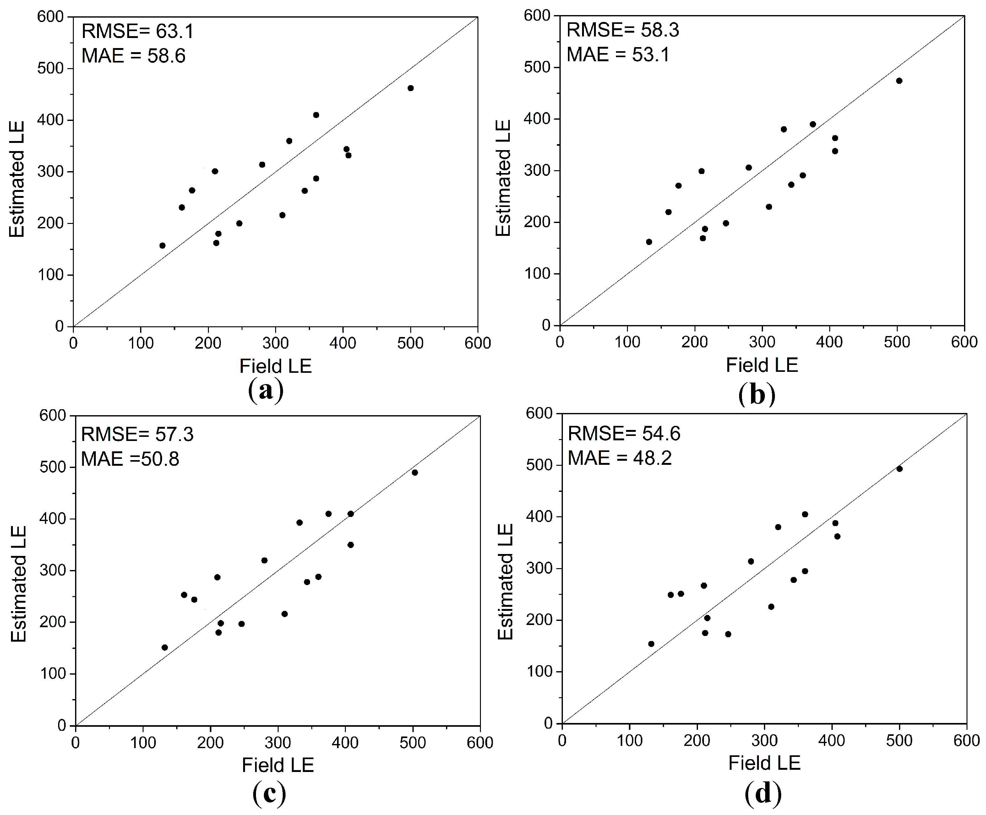
4.2. Performance of Urban Heat Flux Estimations

The in situ measurements from the five sites (B1–B5) listed in Table 1 were used to validate the Landsat TM-retrieved Bowen ratio and latent heat flux. The Bowen ratio maps derived from two remote sensing heat flux models are shown in Figure 8. The LE maps derived from remote sensing heat flux methods are shown in Figure 9. There are obvious spatial differences between the model results using the different retrieved VFCs as driving parameters, particularly in urban regions where some residential evaporation occurred.

Figure 10a,b illustrates the statistical results for all the five sites put together, based on the TSEB model using NDVI-derived VFC and MESMA-derived VFC as the driving parameter, respectively. The statistical results for all the five sites put together, based on the PCACA model using NDVI-derived VFC and MESMA-derived VFC as the driving parameter, respectively, are illustrated in the Figure 10c,d. Furthermore, the differences in heat flux maps based on the PCACA model using the two different VFC sources were relatively similar (see Figure 10g,h), while the TSEB model yielded some substantial differences (see Figure 10e,f).

The spatial patterns of LE are also illustrated along with a histogram that shows the frequency distribution of LE values within the model domain. As shown in Figure 11, different models exhibited different capabilities of capturing the frequency distribution of urban LE estimation. The discrepancies in LE distributions between the two studied models, in terms of both overall magnitude and spatial differences, were larger in urban regions relative to those in non-urban regions. The distributions of the modeled LE results are similar in non-urban areas, with overall bias values of 7.3 Wm⁻² and 4.0 Wm⁻² based on the TSEB model and PCACA model, respectively. However, a larger difference was observed in urban regions, with overall bias values of 58.8 Wm⁻² and 13.9 Wm⁻² based on the TSEB model and PCACA model, respectively. The deviations in the estimated urban LE obtained from both TSEB and PCACA models could be attributed to the differences in the response to urban VFC retrieval. For the TSEB approach, VFC was a critical factor that dominated the pixel-level-combined heat flux. While for the PCACA model, these uncertainties were caused by the spatial context between VFC and LST. This further demonstrated that accurate VFC data is particularly important in enhancing the estimation of urban heat fluxes. Similar finding was observed in the study of [57], which used Surface Urban Energy and Water Balance model to delineate neighborhood scale energy components and demonstrated the importance of vegetative cover in simulating urban energy terms.

Based on Landsat TM/ETM data, latent heat fluxes on 17 April 2001, 12 April 2002, 6 July 2004, 6 May 2005, 22 May 2005, 27 March 2008, 14 May 2008, 2 April 2010, 5 June 2010 and 21 June 2010 were further calculated and analyzed. Since only one or two stations were available per image for the BA1–BA8 sites, these additional images and field data were only used for a single accuracy comparison analysis. It should be noted that, for sites BA1–BA8, there is one or more available images that could be used. Comparisons of the estimated LE with measured fluxes are shown in Figure 12.

It is observed that RMSE value was 63.1 Wm⁻² for TSEB model when using the NDVI-derived VFC, while this value was 58.3 Wm⁻² for PCACA model. The MAE value was 58.6 Wm⁻² for TSEB model when using NDVI-derived VFC; and this value was 53.1 Wm⁻² for PCACA model. On the other hand, when using MESMA-derived VFC, the RMSE of LE was 57.3 Wm⁻² for TSEB model, while this value was 54.6 Wm⁻² for PCACA model. The MAE value was 50.8 Wm⁻² for TSEB model when using MESMA-derived VFC; and this value was 48.2 Wm⁻² for PCACA model.

We also checked the determination coefficients (R²) of the fields with respect to the combination of B1–B5 sites and BA1–BA8 sites. The R² was 0.66 and 0.70 for TSEB model when using the NDVI-derived VFC and MESMA-derived VFC, respectively. Concerning the PCACA model, the R² values for the resultant LE values were 0.72 and 0.73 for the NDVI-derived VFC and the MESMA-derived VFC respectively. Overall, results demonstrated that LE was produced with obvious errors when using the NDVI-derived VFC while this was improved when using the SMA-derived VFC.

5. Discussion

When combined with medium-resolution spatial and spectral features, MESMA-derived method achieved more accurate VFC values in complex urban regions than NDVI-derived method. In particular, the NDVI-derived approach obviously underestimates low VFC areas as compared to estimates using the MESMA approach, especially in complex urban regions where partial cover conditions are more prevalent. This underestimation is mainly associated with the complexity of bare land (bare soil and impervious surfaces) spectra. For the sparsely vegetated areas, the performance of the NDVI-derived method decreases because NDVI is more sensitive to vegetation spectra over high-level bare land areas. This finding is supported by previous studies [58,59] that reported relatively lower vegetation coverages in metropolitan areas (Phoenix and Manaus) would result in estimation difficulties. It should be stressed that for a substantial part of urban thermal studies, the NDVI-derived method was commonly used due to its simplicity and ease of implementation. However, based on the above context, MESMA-derived VFC was found more prospective in studies of urban thermal environments.

Through the investigation we could see that the LE differences between two VFC sources were obvious in local urbanized regions, especially in areas with high-intensity impervious surface pixels (low-intensity urban vegetation) for which only a smaller fraction of the energy translates into evaporation and transpiration. In some regions such as the city center and the southern portions of built-up areas in Beijing, LE was detected using the MESMA-retrieved VFC and was ignored based on the NDVI-retrieved VFC. This can be attributed to the fact that VFC was more likely to be underestimated using the NDVI-derived method in sparsely vegetated areas dominated by light impervious surfaces and soil. In particular, when NDVI-derived VFC was used as input data, latent heat flux was seriously underestimated and even considered as non-existent over high-level impervious surfaces (VFC less than 10%).

Clear dissimilarities were also observed in the frequency distributions of LE estimates between those of TSEB and PCACA models using the same VFC in urban and non-urban regions. Moreover, the discrepancies in the TSEB model-retrieved heat flux values using MESMA VFC versus NDVI VFC inputs were nearly one to two times larger than those of the PCACA model. This may be because that PCACA model could partially counteract the effects of miscalculated VFC on LE estimations using the constraint of spatial context of them. The results of our study are supported by some previous studies [18,60], which have reported that the VFC-LST methodology could be used in complex urban scenes and produce acceptable results.

On the other hand, although previous studies have focused on the validation and applicability of remote sensing-based urban heat flux models, there is no comparative analysis regarding different urban heat flux models. In present study, PCACA model, a typical VFC-LST based trapezoid model that does not require a large number of relative parameters which cannot be retrieved by remote sensing, can be more suitable to delineate urban surface LE and with higher accuracy. In addition, while the TSEB and PCACA models provided acceptable performances with the available remote sensing and meteorological data, the applications of these models needs to be further assessed by invalidating with other experimental sites (i.e., URBANFLUXES (http://urbanfluxes.eu/)) or comparing with other urban energy models. Some effectively neighborhood scale urban climates models, such as [61], should be considered in further work.

6. Conclusions

This study investigated the fractional abundance of urban vegetation based on the heterogeneous pixels of Landsat imagery. A comparative analysis between NDVI-derived and MESMA-derived urban VFC illustrated that the latter achieved more accurate VFC values in complex urban regions. Moreover, MESMA-derived VFC could result in more accurate urban LE estimates relative to NDVI-derived VFC when used as input to both the TSEB and PCACA models. Our study suggests that the MESMA-retrieved VFC, which has not been sufficiently investigated in previous urban thermal environment studies, should be given more attention.

When using the different remote sensing-based VFC driver maps, PCACA model produced smaller differences on the output LE maps over both urban and non-urban regions. However, obvious bias was observed using the TSEB model in both urban and non-urban regions, particularly in the former. Accordingly, PCACA model may be an alternative for remote sensing-based urban heat flux studies that focus on quantitative comparative analyses in complex study regions.

References

1. Grimmond, C.S.B.; Blackett, M.; Best, M.J.; Barlow, J.; Baik, J.; Belcher, S.E.; Bohnenstengel, S.I.; Calmet, I.; Chen, F.; Dandou, A. The international urban energy balance models comparison project: First results from phase 1. J. Appl. Meteorol. Climatol. 2010, 49, 1268–1292. [Google Scholar] [CrossRef]
2. Grimmond, C.S.B.; Blackett, M.; Best, M.J.; Baik, J.J.; Belcher, S.E.; Beringer, J.; Bohnenstengel, S.I.; Calmet, I.; Chen, F.; Coutts, A.M. Initial results from phase 2 of the international urban energy balance model comparison. Int. J. Climatol. 2011, 31, 244–272. [Google Scholar] [CrossRef]
3. Frey, C.M.; Parlow, E.; Vogt, R.; Harhash, M.; Abdel Wahab, M.M. Flux Measurements in Cairo. Part 1: In situ measurements and their applicability for comparison with satellite data. Int. J. Climatol. 2011, 31, 218–231. [Google Scholar] [CrossRef]
4. Frey, C.M.; Parlow, E. Flux Measurements in Cairo. Part 2: On the Determination of the Spatial Radiation and Energy Balance Using ASTER Satellite Data. Remote Sens. 2012, 4, 2635. [Google Scholar] [CrossRef]
5. Kato, S.; Yamaguchi, Y. Estimation of storage heat flux in an urban area using ASTER data. Remote Sens. Environ. 2007, 110, 1–17. [Google Scholar] [CrossRef]
6. Chakraborty, S.D.; Kant, Y.; Mitra, D. Assessment of land surface temperature and heat fluxes over Delhi using remote sensing data. J. Environ. Manag. 2015, 148, 143–152. [Google Scholar] [CrossRef] [PubMed]
7. Kato, S.; Yamaguchi, Y. Analysis of urban heat-island effect using ASTER and ETM+ Data: Separation of anthropogenic heat discharge and natural heat radiation from sensible heat flux. Remote Sens. Environ. 2005, 99, 44–54. [Google Scholar] [CrossRef]
8. Jia, Z.; Liu, S.; Xu, Z.; Chen, Y.; Zhu, M. Validation of remotely sensed evapotranspiration over the Hai River Basin, China. J. Geophys. Res. Atmos. 2012, 117, 13113. [Google Scholar] [CrossRef]
9. Su, Z. The Surface Energy Balance System (SEBS) for estimation of turbulent heat fluxes. Hydrol. Earth Syst. Sci. Discuss. 2002, 6, 85–100. [Google Scholar] [CrossRef]
10. Choi, M.; Kustas, W.P.; Anderson, M.C.; Allen, R.G.; Li, F.; Kjaersgaard, J.H. An intercomparison of three remote sensing-based surface energy balance algorithms over a corn and soybean production region (Lowa, U.S.) during SMACEX. Agric. For. Meteorol. 2009, 149, 2082–2097. [Google Scholar] [CrossRef]
11. Gao, Y.; Long, D. Intercomparison of remote sensing-based models for estimation of evapotranspiration and accuracy assessment based on SWAT. Hydrol. Process. 2008, 22, 4850–4869. [Google Scholar] [CrossRef]
12. Timmermans, W.J.; Kustas, W.P.; Anderson, M.C.; French, A.N. An intercomparison of the surface energy balance algorithm for land (SEBAL) and the two-source energy balance (TSEB) modeling schemes. Remote Sens. Environ. 2007, 108, 369–384. [Google Scholar] [CrossRef]
13. Li, F.; Kustas, W.P.; Prueger, J.H.; Neale, C.M.U.; Jackson, T.J. Utility of Remote Sensing-Based Two-Source Energy Balance Model under low- and high-vegetation cover conditions. J. Hydrometeorol. 2005, 6, 878–891. [Google Scholar] [CrossRef]
14. Weng, Q.; Hu, X.; Quattrochi, D.A.; Liu, H. Assessing Intra-Urban Surface Energy Fluxes Using Remotely Sensed ASTER Imagery and Routine Meteorological Data: A Case Study in Indianapolis, USA. IEEE J. Sel. Top. Appl. Earth Obs. Remote Sens. 2014, 7, 4046–4057. [Google Scholar] [CrossRef]
15. Wong, M.S.; Yang, J.; Nichol, J.; Weng, Q.; Menenti, M.; Chan, P.W. Modeling of Anthropogenic Heat Flux Using HJ-1B Chinese Small Satellite Image: A Study of Heterogeneous Urbanized Areas in Hong Kong. IEEE Geosci. Remote Sens. Lett. 2015, 12, 1466–1470. [Google Scholar] [CrossRef]
16. Zhang, R.; Sun, X.; Wang, W.; Xu, J.; Zhu, Z.; Tian, J. An operational two-layer remote sensing model to estimate surface flux in regional scale: Physical background. Sci. China Ser. D Earth Sci. 2005, 48, 225–244. [Google Scholar]
17. Zhang, R.; Tian, J.; Su, H.; Sun, X.; Chen, S.; Xia, J. Two improvements of an operational two-layer model for terrestrial surface heat flux retrieval. Sensors 2008, 8, 6165–6187. [Google Scholar] [CrossRef] [PubMed]
18. Kuang, W.; Dou, Y.; Zhang, C.; Chi, W.; Liu, A.; Liu, Y.; Zhang, R.; Liu, J. Quantifying the heat flux regulation of metropolitan land use/land cover components by coupling remote sensing modeling with in situ measurement. J. Geophys. Res. Atmos. 2015, 120, 113–130. [Google Scholar] [CrossRef]
19. Yang, Y.; Shang, S. A hybrid dual-source scheme and trapezoid framework—Based evapotranspiration model (HTEM) using satellite images: Algorithm and model test. J. Geophys. Res. Atmos. 2013, 118, 2284–2300. [Google Scholar] [CrossRef]
20. Long, D.; Singh, V.P. A Two-source Trapezoid Model for Evapotranspiration (TTME) from satellite imagery. Remote Sens. Environ. 2012, 121, 370–388. [Google Scholar] [CrossRef]
21. Yang, Y.; Su, H.; Zhang, R.; Tian, J.; Li, L. An enhanced two-source evapotranspiration model for land (ETEML): Algorithm and evaluation. Remote Sens. Environ. 2015, 168, 54–65. [Google Scholar] [CrossRef]
22. Zhang, Y.; Balzter, H.; Wu, X. Spatial-temporal patterns of urban anthropogenic heat discharge in Fuzhou, China, observed from sensible heat flux using Landsat TM/ETM+ data. Int. J. Remote Sens. 2013, 34, 1459–1477. [Google Scholar] [CrossRef]
23. Gibson, L.; Münch, Z.; Engelbrecht, J. Particular uncertainties encountered in using a pre-packaged SEBS model to derive evapotranspiration in a heterogeneous study area in South Africa. Hydrol. Earth Syst. Sci. 2011, 15, 295–310. [Google Scholar] [CrossRef]
24. Kustas, W.P.; Norman, J.M. Evaluating the Effects of Subpixel Heterogeneity on Pixel Average Fluxes. Remote Sens. Environ. 2000, 74, 327–342. [Google Scholar] [CrossRef]
25. Jia, K.; Liang, S.; Gu, X.; Baret, F.; Wei, X.; Wang, X.; Yao, Y.; Yang, L.; Li, Y. Fractional vegetation cover estimation algorithm for Chinese GF-1 wide field view data. Remote Sens. Environ. 2016, 177, 184–191. [Google Scholar] [CrossRef]
26. Chen, Y.; Shi, P.; Li, X.; Jin, C.; Jing, L. A combined approach for estimating vegetation cover in urban/suburban environments from remotely sensed data. Comput. Geosci. 2006, 32, 1299–1309. [Google Scholar]
27. Xiao, J.; Moody, A. A comparison of methods for estimating fractional green vegetation cover within a desert-to-upland transition zone in central New Mexico, USA. Remote Sens. Environ. 2005, 98, 237–250. [Google Scholar] [CrossRef]
28. Gutman, G.; Ignatov, A. The derivation of the green vegetation fraction from NOAA/AVHRR data for use in numerical weather prediction models. Int. J. Remote Sens. 1998, 19, 1533–1543. [Google Scholar] [CrossRef]
29. Maimaitiyiming, M.; Ghulam, A.; Tiyip, T.; Pla, F.; Latorre-Carmona, P.; Halik, Ü.; Sawut, M.; Caetano, M. Effects of green space spatial pattern on land surface temperature: Implications for sustainable urban planning and climate change adaptation. ISPRS J. Photogramm. Remote Sens. 2014, 89, 59–66. [Google Scholar] [CrossRef]
30. Essa, W.; Verbeiren, B.; van der Kwast, J.; Van de Voorde, T.; Batelaan, O. Evaluation of the DisTrad thermal sharpening methodology for urban areas. Int. J. Appl. Earth Obs. Geoinf. 2012, 19, 163–172. [Google Scholar] [CrossRef]
31. Huete, A.; Liu, H.; Batchily, K.; Van Leeuwen, W. A comparison of vegetation indices over a global set of TM images for EOS-MODIS. Remote Sens. Environ. 1997, 59, 440–451. [Google Scholar] [CrossRef]
32. Montandon, L.; Small, E. The impact of soil reflectance on the quantification of the green vegetation fraction from NDVI. Remote Sens. Environ. 2008, 112, 1835–1845. [Google Scholar] [CrossRef]
33. Eastwood, J.; Yates, M.; Thomson, A.; Fuller, R. The reliability of vegetation indices for monitoring saltmarsh vegetation cover. Int. J. Remote Sens. 1997, 18, 3901–3907. [Google Scholar] [CrossRef]
34. Gitelson, A.A. Wide Dynamic Range Vegetation Index for Remote Quantification of Biophysical Characteristics of Vegetation. J. Plant Physiol. 2004, 161, 165–173. [Google Scholar] [CrossRef] [PubMed]
35. Wardlow, B.D.; Egbert, S.L.; Kastens, J.H. Analysis of time-series MODIS 250 m vegetation index data for crop classification in the US Central Great Plains. Remote Sens. Environ. 2007, 108, 290–310. [Google Scholar] [CrossRef]
36. Somers, B.; Asner, G.P.; Tits, L.; Coppin, P. Endmember variability in Spectral Mixture Analysis: A review. Remote Sens. Environ. 2011, 115, 1603–1616. [Google Scholar] [CrossRef]
37. Small, C. Estimation of urban vegetation abundance by spectral mixture analysis. Int. J. Remote Sens. 2001, 22, 1305–1334. [Google Scholar] [CrossRef]
38. Wu, C. Normalized spectral mixture analysis for monitoring urban composition using ETM+ imagery. Remote Sens. Environ. 2004, 93, 480–492. [Google Scholar] [CrossRef]
39. Song, C. Spectral mixture analysis for subpixel vegetation fractions in the urban environment: How to incorporate endmember variability? Remote Sens. Environ. 2005, 95, 248–263. [Google Scholar] [CrossRef]
40. Patino, J.E.; Duque, J.C. A review of regional science applications of satellite remote sensing in urban settings. Comput. Environ. Urban Syst. 2013, 37, 1–17. [Google Scholar] [CrossRef]
41. Weng, Q. Thermal infrared remote sensing for urban climate and environmental studies: Methods, applications, and trends. ISPRS J. Photogramm. Remote Sens. 2009, 64, 335–344. [Google Scholar] [CrossRef]
42. Liu, S.; Hu, G.; Lu, L.; Mao, D. Estimation of Regional Evapotranspiration by TM/ETM+ Data over Heterogeneous Surfaces. Photogramm. Eng. Remote Sens. 2007, 73, 1169–1178. [Google Scholar] [CrossRef]
43. Liu, S.M.; Xu, Z.W.; Zhu, Z.L.; Jia, Z.Z.; Zhu, M.J. Measurements of evapotranspiration from eddy-covariance systems and large aperture scintillometers in the Hai River Basin, China. J. Hydrol. 2013, 487, 24–38. [Google Scholar] [CrossRef]
44. Cooley, T.; Anderson, G.; Felde, G.; Hoke, M.; Ratkowski, A.; Chetwynd, J.; Gardner, J.; Adler-Golden, S.; Matthew, M.; Berk, A. FLAASH, a MODTRAN4-based atmospheric correction algorithm, its application and validation. In Proceedings of the IEEE International Geoscience and Remote Sensing Symposium (IGARSS’02), Toronto, ON, Canada, 24–28 June 2002; pp. 1414–1418. [Google Scholar]
45. Jiménez-Muñoz, J.C.; Sobrino, J.A. A generalized single-channel method for retrieving land surface temperature from remote sensing data. J. Geophys. Res. Atmos. 2003, 108. [Google Scholar] [CrossRef]
46. Valor, E.; Caselles, V. Mapping land surface emissivity from NDVI: Application to European, African, and South American areas. Remote Sens. Environ. 1996, 57, 167–184. [Google Scholar] [CrossRef]
47. Li, X.K.; Wu, T.X.; Liu, K.; Li, Y.; Zhang, L.F. Evaluation of the Chinese Fine Spatial Resolution Hyperspectral Satellite TianGong-1 in Urban Land-Cover Classification. Remote Sens. 2016, 8, 438. [Google Scholar] [CrossRef]
48. Li, X.; Chen, Y.; Shi, P.; Chen, J. Detecting vegetation fractional coverage of typical steppe in Northern China based on multi-scale remotely sensed data. Acta Bot. Sin. 2002, 45, 1146–1156. [Google Scholar]
49. Franke, J.; Roberts, D.A.; Halligan, K.; Menz, G. Hierarchical multiple endmember spectral mixture analysis (MESMA) of hyperspectral imagery for urban environments. Remote Sens. Environ. 2009, 113, 1712–1723. [Google Scholar] [CrossRef]
50. Powell, R.L.; Roberts, D.A.; Dennison, P.E.; Hess, L.L. Sub-pixel mapping of urban land cover using multiple endmember spectral mixture analysis: Manaus, Brazil. Remote Sens. Environ. 2007, 106, 253–267. [Google Scholar] [CrossRef]
51. Roberts, D.A.; Gardner, M.; Church, R.; Ustin, S.; Scheer, G.; Green, R. Mapping chaparral in the Santa Monica Mountains using multiple endmember spectral mixture models. Remote Sens. Environ. 1998, 65, 267–279. [Google Scholar] [CrossRef]
52. Ridd, M.K. Exploring a V-I-S (vegetation-impervious surface-soil) model for urban ecosystem analysis through remote sensing: Comparative anatomy for cities. Int. J. Remote Sens. 1995, 16, 2165–2185. [Google Scholar] [CrossRef]
53. Kustas, W.P.; Norman, J.M. Evaluation of soil and vegetation heat flux predictions using a simple two-source model with radiometric temperatures for partial canopy cover. Agric. For. Meteorol. 1999, 94, 13–29. [Google Scholar] [CrossRef]
54. Lu, L.; Liu, S.; Xu, Z.; Yang, K.; Cai, X.; Jia, L.; Wang, J. The characteristics and parameterization of aerodynamic roughness length over heterogeneous surfaces. Adv. Atmos. Sci. 2009, 26, 180–190. [Google Scholar] [CrossRef]
55. Al-Jiboori, M.H.; Fei, H. Surface roughness around a 325-m meteorological tower and its effect on urban turbulence. Adv. Atmos. Sci. 2005, 22, 595–605. [Google Scholar] [CrossRef]
56. Su, H.-B.; Zhang, R.-H.; Tang, X.-Z.; Sun, X.-M.; Zhu, Z.-L.; Liu, Z.-M. A simplified method to separate latent and sensible heat fluxes using remotely sensed data. In Proceedings of the IEEE International Geoscience and Remote Sensing Symposium (IGARSS’01), Sydney, Ausralia, 9–13 July 2001; pp. 3175–3177. [Google Scholar]
57. Alexander, P.J.; Mills, G.; Fealy, R. Using LCZ data to run an urban energy balance model. Urban Clim. 2015, 13, 14–37. [Google Scholar] [CrossRef]
58. Myint, S.W.; Okin, G.S. Modelling land-cover types using multiple endmember spectral mixture analysis in a desert city. Int. J. Remote Sens. 2009, 30, 2237–2257. [Google Scholar] [CrossRef]
59. Okin, G.S.; Roberts, D.A.; Murray, B.; Okin, W.J. Practical limits on hyperspectral vegetation discrimination in arid and semiarid environments. Remote Sens. Environ. 2001, 77, 212–225. [Google Scholar] [CrossRef]
60. Amiri, R.; Weng, Q.; Alimohammadi, A.; Alavipanah, S.K. Spatial-temporal dynamics of land surface temperature in relation to fractional vegetation cover and land use/cover in the Tabriz urban area, Iran. Remote Sens. Environ. 2009, 113, 2606–2617. [Google Scholar] [CrossRef]
61. Alexander, P.J.; Bechtel, B.; Chow, W.T.L.; Fealy, R.; Mills, G. Linking urban climate classification with an urban energy and water budget model: Multi-site and multi-seasonal evaluation. Urban Clim. 2016, 17, 196–215. [Google Scholar] [CrossRef]
Figure 1. The left is the location of study areas in the China. The right map is the Landsat 5 TM true color composition imagery of Beijing, overlaid with the field measurements and meteorological station sites (listed in Table 1).
Remotesensing 09 00455 g001
Figure 2. The overall flowchart of this study. The solid blue box represents the input data. From top to bottom, the dashed red boxes illustrate image pre-processing, model implementation and analysis of results.
Remotesensing 09 00455 g002
Figure 3. Illustration of the spectra endmembers with different numbers of clusters: (a) 11 for vegetation; (b) 5 for bare soil; (c) 6 for high-albedo impervious surfaces; and (d) 6 for low-albedo impervious surfaces.
Remotesensing 09 00455 g003
Figure 4. The trapezoid of vegetation fractional cover/land surface temperature (VFC/LST) space, in which v and s denote vegetated areas and bare ground, respectively, and d and w denote extremely dry and extremely wet areas, respectively.
Remotesensing 09 00455 g004
Figure 5. The VFC maps based on: (a) Normalized Difference Vegetation Index (NDVI)-derived method; and (b) Multiple Endmember Spectral Mixture Analysis (MESMA)-derived method. Detailed VFC maps in the urban region (blue box) based on: (c) NDVI-derived method; and (d) MESMA-derived method.
Remotesensing 09 00455 g005
Figure 6. Scatter plots of estimated VFC versus reference VFC based on the: (a) NDVI-derived method; and (b) MESMA-derived method. Red circles exhibited the difference over the relatively low VFC range.
Remotesensing 09 00455 g006
Figure 7. Normalized frequency plots of the two estimated VFCs in: (a) urban regions; and (b) non-urban regions (Note that the x-axis is from 0.02 to 0.98).
Remotesensing 09 00455 g007
Figure 8. Bowen ratio maps of the NDVI-derived and MESMA-derived methods based on the PCACA and TSEB models: (a) NDVI–TSEB; (b) MESMA–TSEB; (c) NDVI–PCACA; and (d) MESMA–PCACA.
Remotesensing 09 00455 g008
Figure 9. LE maps (in Wm−2) based on the NDVI-derived and MESMA-derived methods and the PCACA and TSEB models: (a) NDVI–TSEB; (b) MESMA–TSEB; (c) NDVI–PCACA; and (d) MESMA–PCACA.
Remotesensing 09 00455 g009
Figure 10. Comparisons of estimated Bowen ratio and LE (in Wm−2) with measured Bowen ratio and LE by the flux towers B1–B5 (listed on Table 1): (a,e) NDVI–TSEB; (b,f) MESMA–TSEB; (c,g) NDVI–PCACA; and (d,h) MESMA–PCACA.
Remotesensing 09 00455 g010
Figure 11. Frequency plots of estimated LE data based on the NDVI-derived and MESMA-derived models: (a,c) urban region; and (b,d) non-urban region.
Remotesensing 09 00455 g011
Figure 12. Scatter plots of estimated and measured LE (in Wm−2) by the flux towers BA1-BA8 (listed on Table 1): (a) NDVI–TSEB; (b) MESMA–TSEB; (c) NDVI–PCACA; and (d) MESMA–PCACA.
Remotesensing 09 00455 g012