Sea Wind Measurement by Doppler Navigation System with X-Configured Beams in Rectilinear Flight

Abstract

We suggest a conceptual approach to the measurement of the near-surface wind vector over water using a Doppler navigation system, in addition to its standard navigation capabilities. We consider a Doppler navigation system with a track-stabilized antenna and x-configuration of its beams. For the measurement of the sea-surface wind, the system operates in the multi-beam scatterometer mode in rectilinear flight. The proposed conceptual design has been validated, and its accuracy for the wind vector measurement has been estimated using Monte Carlo computational simulations.

1. Introduction

Applications of modern radars are highly diverse, including remote sensing radars for various observations, air and terrestrial traffic control, radar astronomy, marine navigation systems, aircraft anti-collision systems, ocean surveillance systems, outer space surveillance and rendezvous systems, meteorological precipitation monitoring, altimetry and flight control systems, and range-controlled radar for public health surveillance. High-tech radar systems commonly utilize digital signal processing, machine learning, and are capable of extracting useful information under very high noise levels.

Modern airborne radars are integrated into appropriate avionics systems and provide a powerful tool for observation, navigation, and avoidance solutions [1]. The rapid development of radars leads not only to their integration, but also to the extension of their functionality and applicability [2]. Remote sensing of the water surface and of the near-surface wind appears one of the promising additional applications of airborne radars.

Microwaves are widely used for various remote sensing applications including observation and monitoring of the environment. Near-surface wind measurements over the sea are of immense importance for navigation, meteorology, and operational oceanography.

Microwave backscattering from the water surface has been widely investigated in recent decades [3,4,5,6,7,8,9,10,11,12,13,14,15,16,17,18,19,20,21,22,23,24,25,26]. The typical method for describing the sea clutter is in the form of the normalized radar cross-section (NRCS), the statistical distribution of the NRCS, the amplitude correlation, and the spectral shape of the Doppler returns.

The wind blowing over the sea modifies the surface backscatter properties depending on both wind speed and direction. Wind speed U can be measured by a scatterometer, since a stronger wind produces a larger NRCS ${\sigma }^{\circ }(U,\theta ,\alpha )$ at a medium incidence angle θ, and a smaller NRCS at a small (near nadir) incidence angle. Wind direction can also be assessed, because NRCS varies as a function of the azimuth illumination angle α relative to the up-wind direction [9]. The accuracy of the wind direction scatterometric measurements is about ±20°, while the accuracy of the scatterometric wind speed estimation is typically around ±2 m/s for wind speeds ranging between 3 and 24 m/s.

The relationship between the NRCS and the near-surface wind vector, sometimes called the “geophysical model function”, must be known for the wind retrieval. Scatterometer experiments have shown that this model function for medium incidence angles at given transmitting and receiving polarization (either vertical or horizontal) is represented by [27]:

$${\sigma }^{\circ }(U,\theta ,\alpha )=A(U,\theta )+B(U,\theta )\cos \alpha +C(U,\theta )\cos (2\alpha ),$$

(1)

where $A(U,\theta )$, $B(U,\theta )$, and $C(U,\theta )$ are the Fourier terms that depend on the sea surface wind speed and incidence angle, $A(U,\theta )=a_0(\theta )U^{{\gamma }_0(\theta )}$, $B(U,\theta )=a_1(\theta )U^{{\gamma }_1(\theta )}$, and $C(U,\theta )=a_2(\theta )U^{{\gamma }_2(\theta )}$; $a_0(\theta )$, $a_1(\theta )$, $a_2(\theta )$, ${\gamma }_0(\theta )$, ${\gamma }_1(\theta )$, and ${\gamma }_2(\theta )$ are the coefficients dependent on the incidence angle, radar wavelength, and polarization.

A number of successful airborne and platform scatterometer experiments performed for a study of water surface backscattering, its dependence on both the incidence and azimuth angles, frequency, polarization, wind speed, and direction [4,6,7,8,10,18] allowed the development of appropriate geophysical model functions, and to further use them for wind retrieval by satellite and airborne scatterometers. Experimental airborne wind measurements by a scatterometer are typically performed in either circular track flight using a fixed fan-beam antenna or in rectilinear track flight using a rotating antenna. Research scatterometers are typically installed on board as external equipment that commonly worsens aircraft aerodynamics and, as a result, reduces flight characteristics of aircraft. This disadvantage can be resolved by use of the modified conventional navigation instruments of aircraft in a scatterometer mode. Recently, such approach has been considered for airborne weather radar application for wind estimation over water at circular and rectilinear flights [28,29]. In general, rectilinear flight measurements can be performed considerably faster and easier to handle. Therefore, in this paper we consider and summarize the possibilities to enhance functionality of a Doppler navigation system (DNS) in order to apply it for remote sensing of the wind speed and direction over water at a rectilinear flight, in addition to its standard application, e.g., for safe landing of seaplane or amphibious aircraft on water.

2. Materials and Methods

2.1. Doppler Navigation System Functions and Applications

DNS is a self-contained radar system that uses the Doppler effect (Doppler radar) for measuring the ground speed and drift angle of aircraft and performs its dead-reckoning navigation [30]. For a detailed overview of the history of DNSs development we refer to [31]. Detailed description of the Doppler navigation principles and DNS functionality can be found, e.g., in [2,32,33,34].

Except for some heavy precipitation conditions, the DNS is all-weather navigational system operating at any time of day and night continuously providing the aircraft position and speed in any location. A complete DNS consists of the Doppler radar, the heading and vertical references, and the navigation computer. The Doppler radar provides the DNS with the speed information while directional sensors provide it with the directional information. Combining these information components allows determining the along-heading, cross-heading, vertical and ground speeds of aircraft as well as its drift angle. The speed information is continuously integrated into the distance traveled from the departure point to resolve the current position of aircraft. Additionally, setting the destination point information (or the desired course and distance), the DNS provides the autopilot with information on bearing to destination, distance to destination point, track-angle error, and cross-course deviation.

For the airborne DNS, the internationally authorized frequency band of 13.25 to 13.4 GHz has been allocated. A center frequency of 13.325 GHz of the band corresponds to a radar wavelength of 2.25 cm, which is within the Ku-band. This frequency provides a good compromise between the use of lower frequencies, resulting in low-velocity sensitivity and large aircraft antenna size and beamwidths, and the use of higher frequencies, resulting in excessive absorption and backscattering effects of the atmosphere and precipitation [2].

Measuring of both the ground speed and drift angle of aircraft is based on the changes in the Doppler frequency of the signal reflected from the underlying surface, depending on a spatial position of an antenna beam. Typical DNS antenna has three beams (λ-configuration; beams 1, 2, and 3) or four beams (x-configuration; beams 1, 2, 3, and 4) spatially oriented as presented in Figure 1. An effective antenna beamwidth θ_a is typically of 3° to 10° [34]. DNS has the track-stabilized (roll-and-pitch-stabilized) or fixed antenna system. As DNS should operate over water, as well as over land, power reasons and DNS sensitivity to velocity influence the choice of a mounting angle for a beam axis in the vertical plane θ₀.

For most types of terrain, the NRCS decreases slowly with increasing the beam incidence angle. However, for the water surface at its various conditions, the NRCS falls radically as the incidence angle increases and assumes different values for various conditions of the sea state or water roughness. At the typical Doppler-radar incidence angles of 15° to 30° (Figure 2), the NRCS is considerably smaller for most sea states than for land and decreases markedly for the smoother sea state [2]. Thus, a Doppler-radar design is based on the NRCS for the smoothest sea state [34].

Choice of a mounting angle for a beam axis in the horizontal plane Γ₀ depends on the desired sensitivity to drift, which tends to increase with increasing this mounting angle. These mounting angles for Doppler radars are typically of 15° to 45° [34].

Choice of the mounting angle for a beam axis in the inclined plane η₀ (nominal angle between the antenna longitudinal axis and the beam direction) represents a certain compromise between high sensitivity to velocity and over-water accuracy, which increases with smaller mounting angles for a beam axis in the inclined plane, and high signal return over water, which increases at larger mounting angles for a beam axis in the inclined plane. The choice of this mounting angle is also determined by the requirements to the width of the Doppler spectrum of the reflected signal, which depends on the effective antenna beamwidth in this plane. Most DNSs use the mounting angle for a beam axis in the inclined plane of somewhere between 65° and 80° [2].

The relation between these mounting angles is given by the following equation [2,34]:

$$\cos {\eta }_0=\cos {\Gamma }_0\cos {\theta }_0.$$

(2)

As the DNS multi-beam antenna provides the selection of a power backscattered by the underlying surface from significantly different directions corresponding to the appropriate beam relative to the aircraft course ψ, as shown in Figure 1, this feature can be used for the enhancement of its functionality to measure the near-surface wind speed and direction over water in the mode of a multi-beam scatterometer in rectilinear flight.

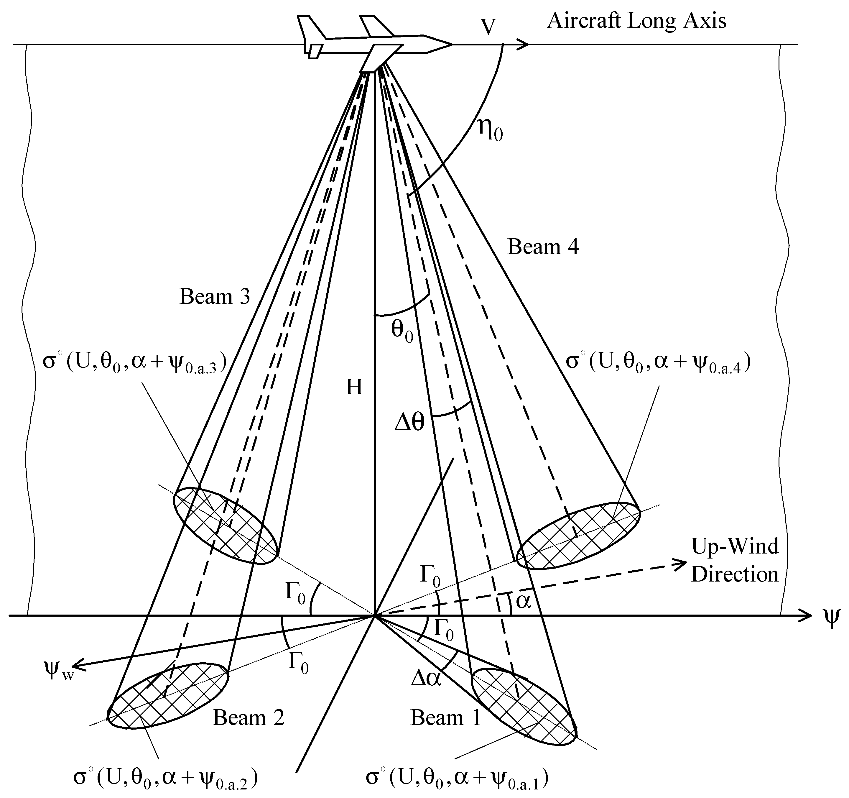
2.2. Near-Surface Wind Measuring

Let an aircraft equipped with the DNS perform a horizontal rectilinear flight with speed V at some altitude H above the mean water surface, the DNS uses a roll-and-pitch-stabilized antenna (physically stabilized to the local horizontal) such that the value of the incidence angle θ remains essentially constant and equal to the chosen design value θ₀. Let the aircraft velocity vector V be located along the intersection of the local horizontal plane and the local vertical plane through the longitudinal axis of the aircraft (that is, the condition for no-drift and no-climb angles), which means that the aircraft is flying horizontally and the aircraft course ψ is the same as the aircraft ground track. The directions of the DNS beams 1, 2, 3, and 4 relative to the aircraft course are ψ_0.a.1, ψ_0.a.2, ψ_0.a.3, and ψ_0.a.4, respectively (Figure 1). Let the wind and wave field be uniform over the scene and the sea-surface wind blow in direction ψ_w, the angle between the up-wind direction and the aircraft course ψ be α, and the NRCS model function for medium incidence angles follows Equation (1). Then, the NRCS values obtained with beams 1, 2, 3, and 4 are ${\sigma }^{\circ }(U,{\theta }_0,\alpha +{\psi }_{0.a.1})$, ${\sigma }^{\circ }(U,{\theta }_0,\alpha +{\psi }_{0.a.2})$, ${\sigma }^{\circ }(U,{\theta }_0,\alpha +{\psi }_{0.a.3})$, and ${\sigma }^{\circ }(U,{\theta }_0,\alpha +{\psi }_{0.a.4})$, respectively, where ${\psi }_{0.a.1}={\Gamma }_0$, ${\psi }_{0.a.2}={180}^{\circ }-{\Gamma }_0$, ${\psi }_{0.a.3}={180}^{\circ }+{\Gamma }_0$, ${\psi }_{0.a.4}={360}^{\circ }-{\Gamma }_0$.

Despite of the fact that the highest mounting angle of a beam axis in the vertical plane of 30° in the range of DNS typical mountings angles requires the biggest transmitted power in comparison with other cases of lower mounting angles in the vertical plane, this incidence angle provides a better usage of the anisotropic properties of the water surface scattering at medium incidence angles to measure the near-surface wind vector as well as to increase the measurement accuracy for typical DNS parameters and angular resolution in the azimuthal plane.

Angular resolution in the azimuthal plane is expressed as:

$$\Delta \alpha =\arctan \left(\frac{\tan (0.5{\theta }_{a.h})}{\sin \theta }\right),$$

(3)

where θ_a.h is the beamwidth in the horizontal plane. Thus, from Equation (3), a 3° beamwidth in the horizontal plane provides an angular resolution in the azimuthal plane of 6.0° at incidence angle of 30°. Alternatively, a beamwidth of 10° in the same plane would provide an azimuthal resolution of 19.9°, which is still acceptable for airborne scatterometer wind measurement as the NRCS model function for medium incidence angles by Equation (1) can be used without any correction in the wind measurement when the azimuth angular size of a cell is up to 15°–20° [35], but a delay selection needs to be used additionally in this case to reduce the selected cell size in the vertical plane.

As the considered DNS antenna is track-stabilized (both roll and pitch stabilized), the values of the incidence angles of beam axes and beam locations in the azimuthal plane remain equal to the given design values at flight, and then the following system of four equations can be written as:

$$\{\begin{array}{l}{\sigma }^{\circ }(U,{\theta }_0,\alpha +{\psi }_{0.a.1})=A(U,{\theta }_0)+B(U,{\theta }_0)\cos (\alpha +{\psi }_{0.a.1})+C(U,{\theta }_0)\cos (2(\alpha +{\psi }_{0.a.1})),\\ {\sigma }^{\circ }(U,{\theta }_0,\alpha +{\psi }_{0.a.2})=A(U,{\theta }_0)+B(U,{\theta }_0)\cos (\alpha +{\psi }_{0.a.2})+C(U,{\theta }_0)\cos (2(\alpha +{\psi }_{0.a.2})),\\ {\sigma }^{\circ }(U,{\theta }_0,\alpha +{\psi }_{0.a.3})=A(U,{\theta }_0)+B(U,{\theta }_0)\cos (\alpha +{\psi }_{0.a.3})+C(U,{\theta }_0)\cos (2(\alpha +{\psi }_{0.a.3})),\\ {\sigma }^{\circ }(U,{\theta }_0,\alpha +{\psi }_{0.a.4})=A(U,{\theta }_0)+B(U,{\theta }_0)\cos (\alpha +{\psi }_{0.a.4})+C(U,{\theta }_0)\cos (2(\alpha +{\psi }_{0.a.4})).\end{array}$$

(4)

To perform the wind retrieval, the system of Equation (4) should be solved approximately using a searching procedure within the ranges of discrete values of possible solutions to recover the wind speed and up-wind direction from the NRCS data set obtained, and then the navigation wind direction can be found as:

$${\psi }_w=\psi -\alpha \pm {180}^{\circ }.$$

(5)

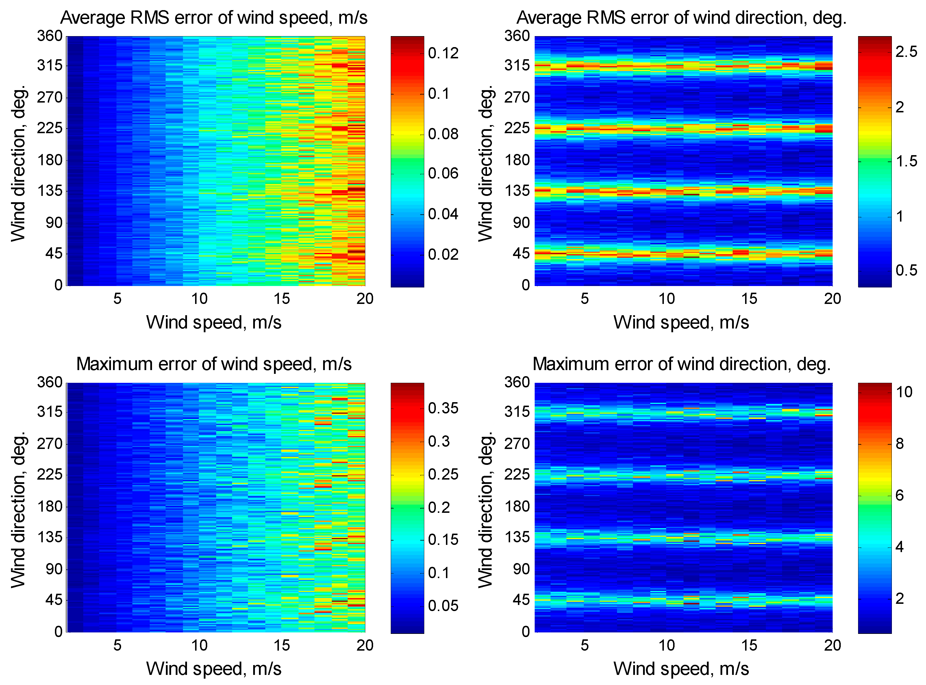
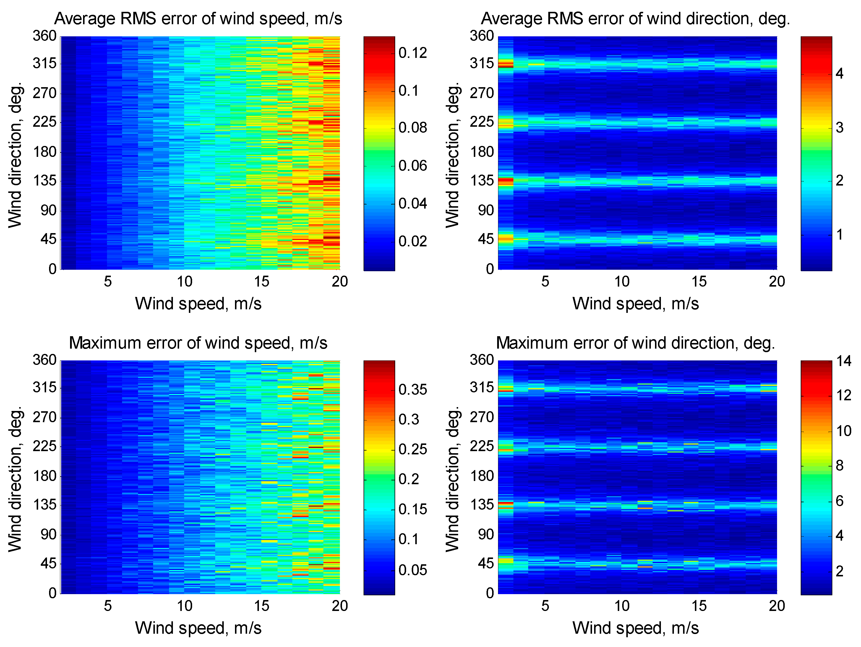
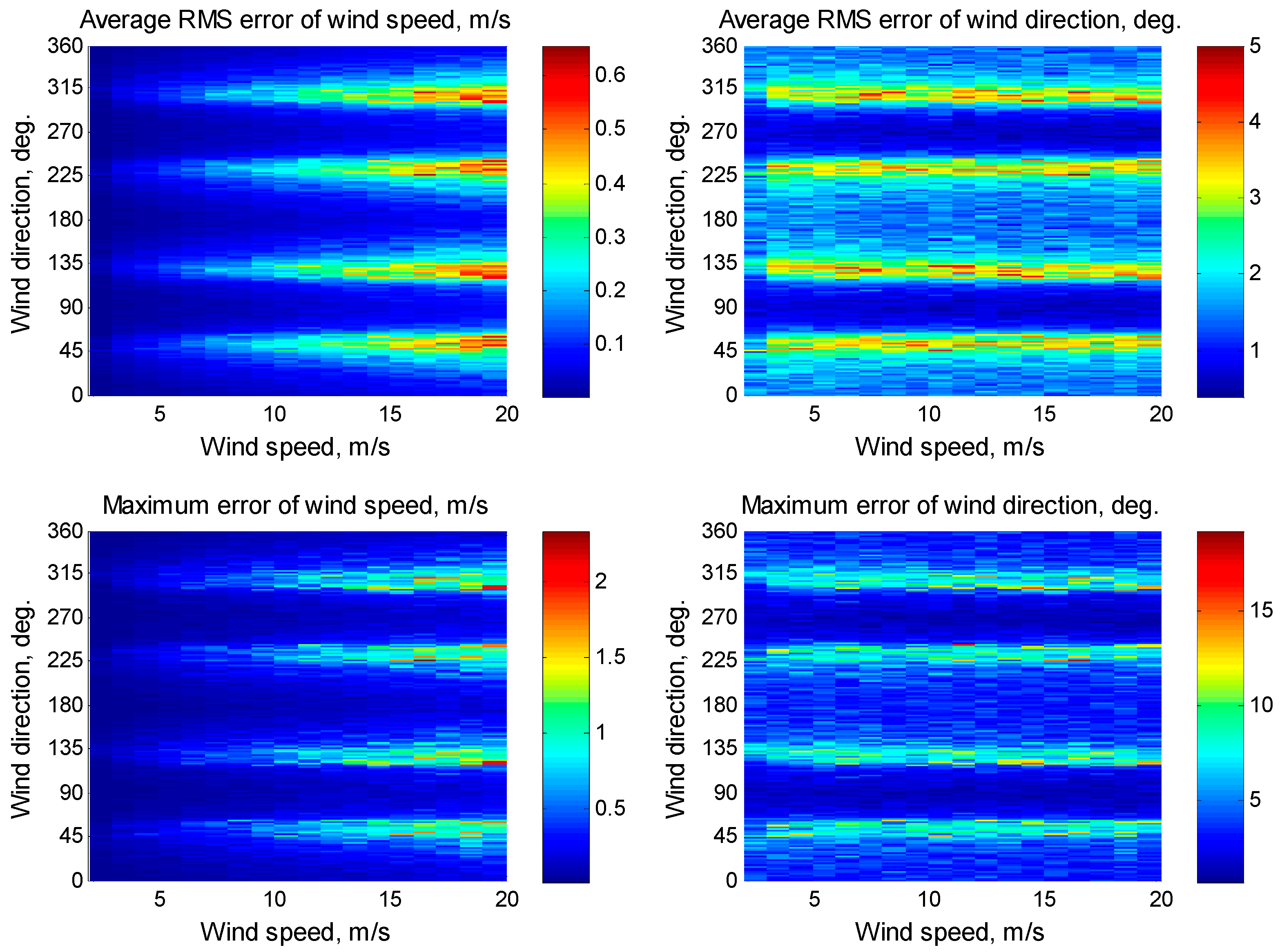
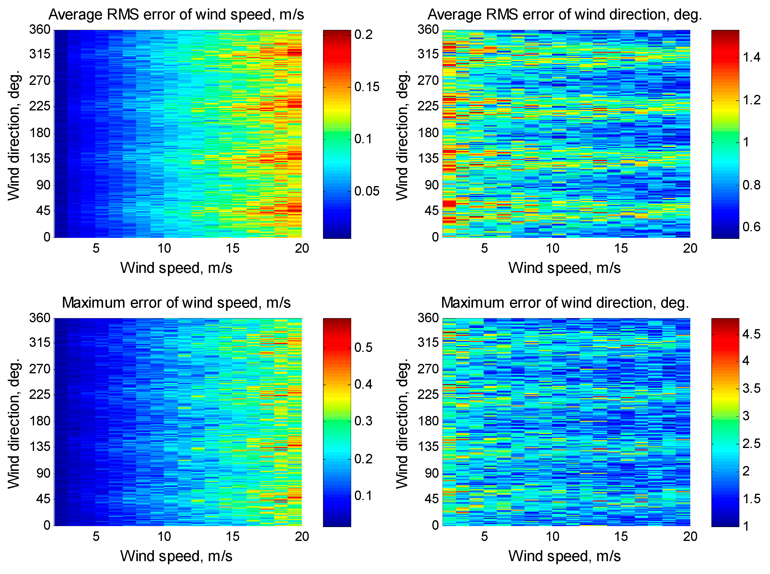
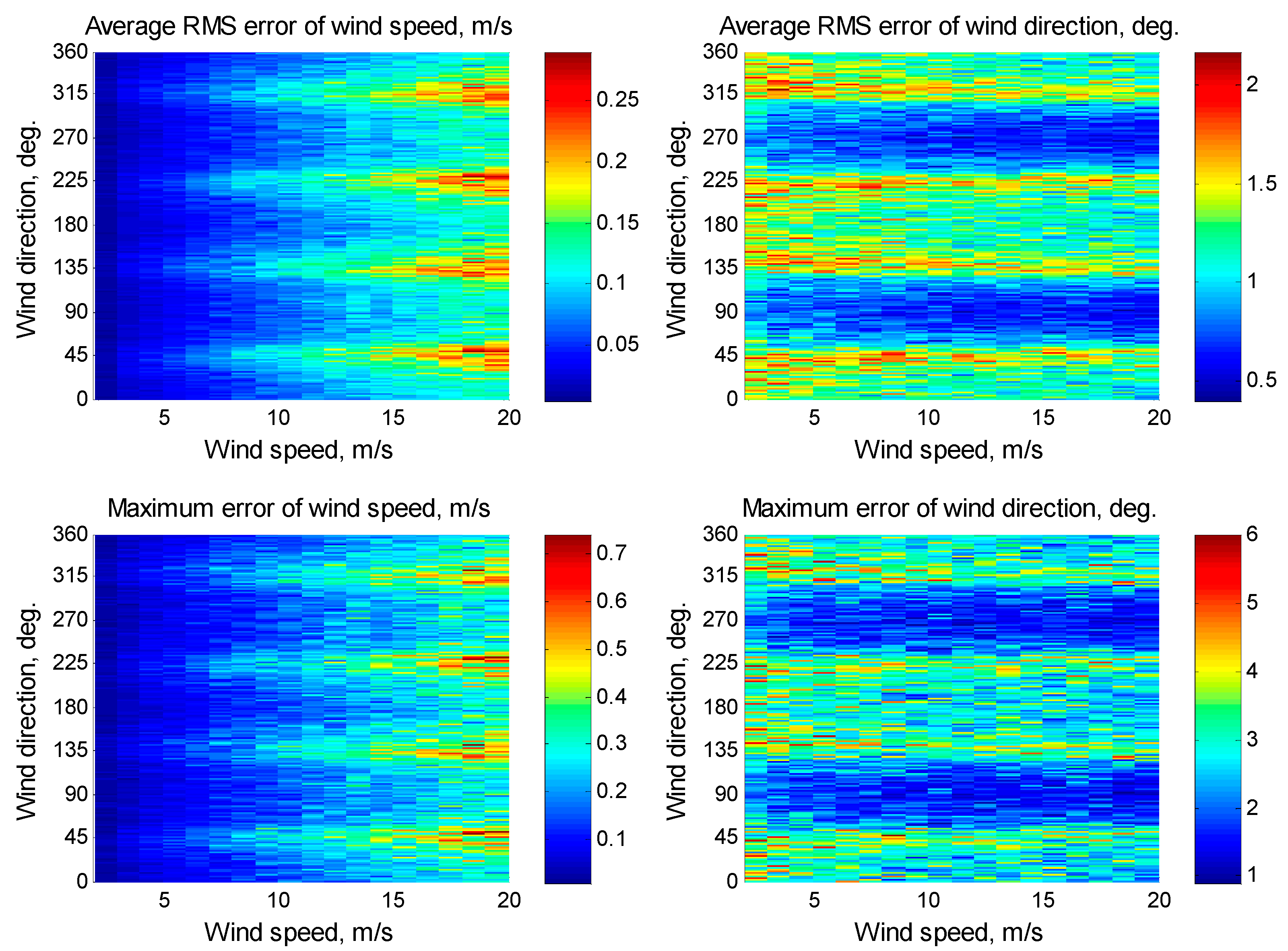
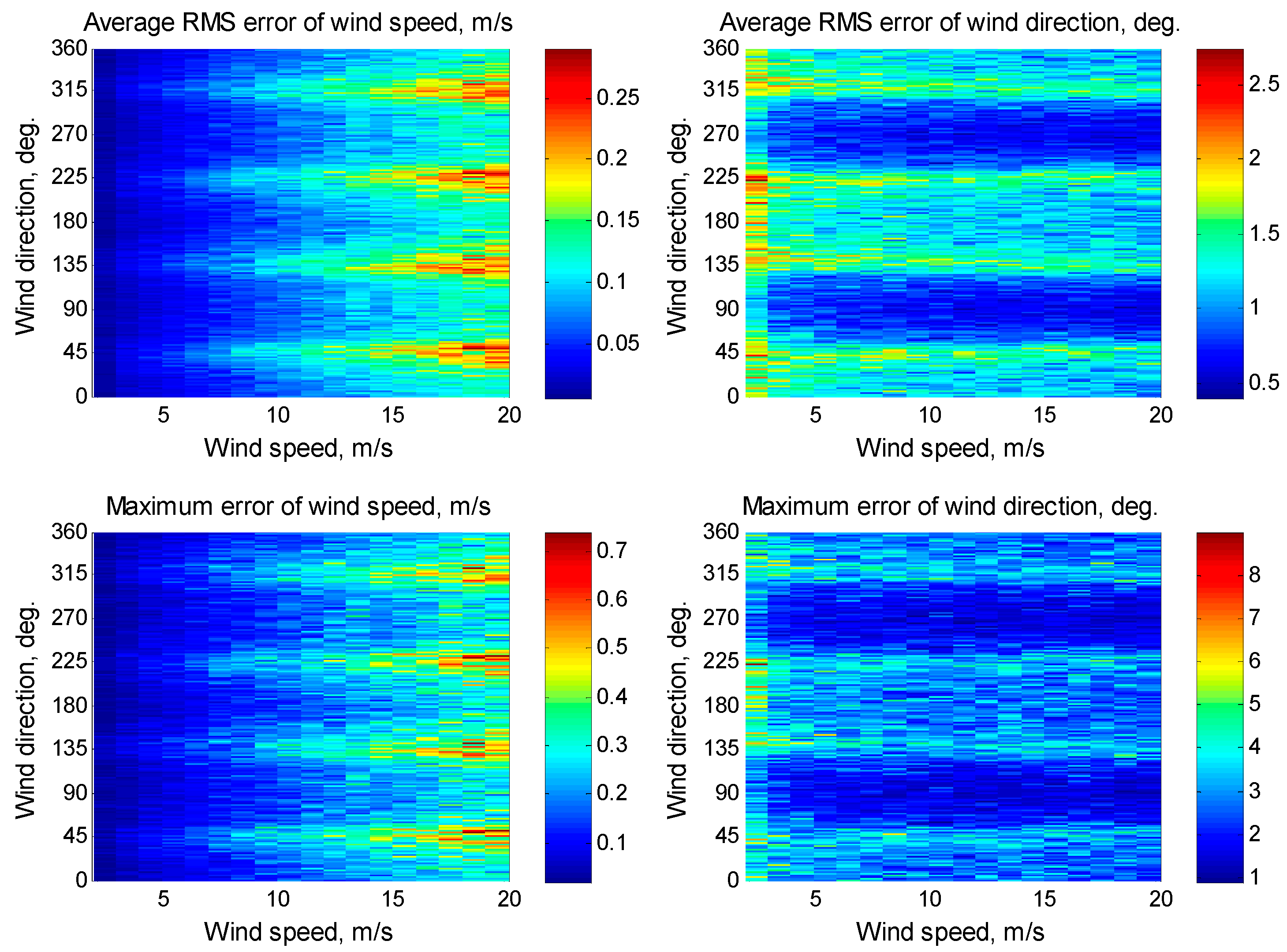
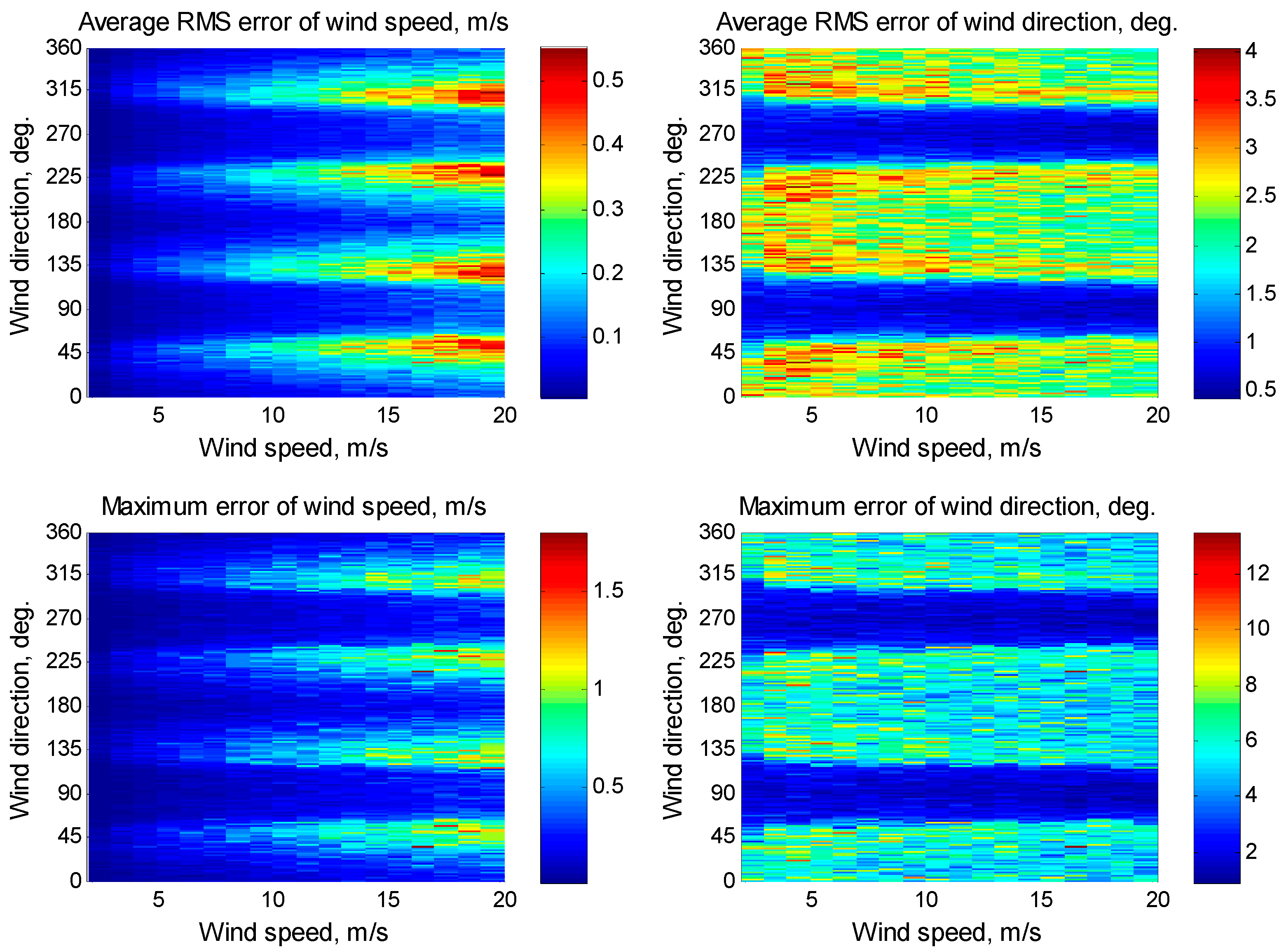
3. Results and Discussion

It has been shown above how the DNS with x-configuration of its beams can be used to measure the near-surface wind speed and direction over water in the mode of a multi-beam scatterometer in rectilinear flight.

DNS in the mode of the multi-beam scatterometer should use the horizontal transmitting and receiving polarization, which provides a greater difference between the upwind and downwind NRCS values than the vertical transmitting and receiving polarization [4,7,36]. As the range of typical mounting angles of a beam axis in the vertical plane (15° to 30°) is not so far from nadir, the highest incidence angle from this range should be used to provide better usage of the anisotropic properties of water surface scattering at medium incidence angles [35]. Additionally, the incidence angle of selected cells should be in the range of validity of the geophysical model functions for medium incidence angles, which is usually between 25°–30° and 55°–60°.

The sea-surface wind measurement by the DNS should be performed in accordance with the following recommendations: The measurement is started when a stable horizontal rectilinear flight at a given altitude and speed of flight has been established. The measurement is finished when the required number of NRCS samples for each beam azimuth observed is obtained. If needed, an additional measurement flight after 45° change of the aircraft course can be performed to verify the results obtained. To obtain a greater number of NRCS samples for each direction observed, several consecutive flights should be performed over the same area with the same course, altitude, and speed of flight.

Based on the data processing, two wind estimation modes can be realized for DNS, namely the normal mode and the fast mode. In the normal mode, the wind retrieval performs by solving the system of Equation (4). In the fast mode, the wind direction can be found using the following inequalities [37]:

$$\begin{gathered} if\left[{\sigma }_{}^{\circ }(U,{\theta }_0,\alpha +{\psi }_{0.a.1})>{\sigma }_{}^{\circ }(U,{\theta }_0,\alpha +{\psi }_{0.a.3})and \\ {\sigma }_{}^{\circ }(U,{\theta }_0,\alpha +{\psi }_{0.a.2})\ge {\sigma }_{}^{\circ }(U,{\theta }_0,\alpha +{\psi }_{0.a.4})\right] \\ or\left[{\sigma }_{}^{\circ }(U,{\theta }_0,\alpha +{\psi }_{0.a.1})\ge {\sigma }_{}^{\circ }(U,{\theta }_0,\alpha +{\psi }_{0.a.3})and \\ {\sigma }_{}^{\circ }(U,{\theta }_0,\alpha +{\psi }_{0.a.2})<{\sigma }_{}^{\circ }(U,{\theta }_0,\alpha +{\psi }_{0.a.4})\right] \\ \Rightarrow {\psi }_w=A_p-\psi -{\Gamma }_0\pm {180}^{\circ }, \\ if\left[{\sigma }_{}^{\circ }(U,{\theta }_0,\alpha +{\psi }_{0.a.1})\le {\sigma }_{}^{\circ }(U,{\theta }_0,\alpha +{\psi }_{0.a.3})and \\ {\sigma }_{}^{\circ }(U,{\theta }_0,\alpha +{\psi }_{0.a.2})>{\sigma }_{}^{\circ }(U,{\theta }_0,\alpha +{\psi }_{0.a.4})\right] \\ or\left[{\sigma }_{}^{\circ }(U,{\theta }_0,\alpha +{\psi }_{0.a.1})<{\sigma }_{}^{\circ }(U,{\theta }_0,\alpha +{\psi }_{0.a.3})and \\ {\sigma }_{}^{\circ }(U,{\theta }_0,\alpha +{\psi }_{0.a.2})\le {\sigma }_{}^{\circ }(U,{\theta }_0,\alpha +{\psi }_{0.a.4})\right] \\ \Rightarrow {\psi }_w=A_p-\psi -{\Gamma }_0, \end{gathered}$$

(6)

where A_p is the principal value of arctangent:

$$A_p=\arctan \left(\frac{\cos ({180}^{\circ }-2{\Gamma }_0)-\frac{{\sigma }^{\circ }(U,{\theta }_0,\alpha +{\psi }_{0.a.2})-{\sigma }^{\circ }(U,{\theta }_0,\alpha +{\psi }_{0.a.4})}{{\sigma }^{\circ }(U,{\theta }_0,\alpha +{\psi }_{0.a.1})-{\sigma }^{\circ }(U,{\theta }_0,\alpha +{\psi }_{0.a.3})}}{\sin ({180}^{\circ }-2{\Gamma }_0)}\right).$$

(7)

Then, the wind speed can be found from the following equation:

$$\begin{gathered} {\sigma }^{\circ }(U,{\theta }_0,\alpha +{\psi }_{0.a.1})+{\sigma }^{\circ }(U,{\theta }_0,\alpha +{\psi }_{0.a.2})+{\sigma }^{\circ }(U,{\theta }_0,\alpha +{\psi }_{0.a.3})+{\sigma }^{\circ }(U,{\theta }_0,\alpha +{\psi }_{0.a.4}) \\ =4A(U,\theta )+4C(U,\theta )\cos (2{\psi }_w+2\psi +{180}^{\circ })\cos (2{\Gamma }_0-{180}^{\circ }). \end{gathered}$$

(8)

The results obtained in the fast mode can be also used as first-order approximations for further, more precise, assessment of the wind vector in the normal mode.

To investigate the capability of the proposed wind algorithm, computer simulations of the wind vector retrieval with DNS having narrow beamwidth were performed for three particular cases of mounting angles of a beam axis in the horizontal plane: 45°, 30°, and 15° (the highest, medium, and lowest angles from the typical range of mounting angles of a beam axis in the horizontal plane), taking into account the random “speckle” and instrumental noise. The Ku-band geophysical model function from [4] has been used for this simulation. The “measured” azimuth NRCS values were generated using a Rayleigh power (exponential) distribution. Monte Carlo simulations with 50 trials at wind speeds of 2 to 20 m/s have been performed to simulate the wind retrieval by solving the system of Equation (4). Search resolutions used in the system of Equation (4) were 0.01 m/s and 0.1° for the wind speed and direction, respectively. Mostly, DNS provides a good signal-to-noise ratio making the noise influence insignificant for measurement results. Nevertheless, the noise influence may affect the wind retrieval errors at lower NRCSs corresponded to lower wind speeds (lower power of backscattered signal from the water surface). In spite of the fact that the scatterometer instrumental measurement noise of 0.2 dB can lead to uncertainty in the wind speed retrieval of 0.5 m/s only [21], it can also cause valuable uncertainties in the wind direction recovery. Thus, the wind retrieval errors have been estimated without and with additive instrumental noise to evaluate the potential applicability of the method in both cases.

First, the simulations have been performed for the incidence angle of 30°, which corresponded to the highest DNS mounting angle of a beam axis in the vertical plane from the range of its typical angles. Five thousand “measured” NRCS samples have been averaged for each azimuthal angle. The simulation results without instrumental noise and with the assumption of 0.1 dB instrumental noise for mounting angles of a beam axis in the horizontal plane of 45°, 30°, and 15° are presented in Figure 3, Figure 4, Figure 5, Figure 6, Figure 7 and Figure 8, respectively. The simulations at the incidence angle of 30° has shown that the maximum errors of the wind speed and direction retrieval for mounting angles of a beam axis in the horizontal plane of 45°, 30°, and 15° without instrumental noise are 0.37 m/s and 10.3°, 0.94 m/s and 11.7°, 2.3 m/s and 19.0°, and with the assumption of 0.1 dB instrumental noise are 0.39 m/s and 14.0°, 0.97 m/s and 14.6°, and 2.4 m/s and 19.6°, respectively. The errors are within the range of typical errors for the scatterometric wind retrieval in all the considered cases for the DNS typical mounting angles of a beam axis in the horizontal plane, but with the exception of the wind speed errors at the worst case of a beam axis in the horizontal plane of 15°. Hence, the best location of the DNS beams in the horizontal plane corresponds to the mounting angle of a beam axis in the horizontal plane of 45°, which provides the lowest wind retrieval errors.

The above examples clearly indicate the suitability of the DNS for the sea wind measurement at the mounting angle of a beam axis in the vertical plane of 30° and the accuracy of the proposed algorithm, with the exception of the worst case of a beam axis in the horizontal plane of 15°.

Nevertheless, another case with higher and an atypical mounting angle of a beam axis in the vertical plane of 45° has also been considered and corresponding simulations have been performed. Our simulations have shown that such a mounting angle in the vertical plane allows obtaining better wind retrieval results than at the typical mounting angle of a beam axis in the vertical plane of 30° even under lower number of averaged “measured” NRCS samples for each azimuthal angle. The simulation results without instrumental noise and with assumption of 0.2 dB instrumental noise for mounting angles of a beam axis in the horizontal plane of 45°, 30°, and 15° with averaging 1565 “measured” NRCS samples are presented in Figure 9, Figure 10, Figure 11, Figure 12, Figure 13 and Figure 14, respectively. The maximum errors of the wind speed and direction retrieval without instrumental noise are 0.57 m/s and 4.8°, 0.73 m/s and 6.0°, and 1.75 m/s and 13.8°, and with the assumption of 0.2 dB instrumental noise are 0.58 m/s and 7.7°, 0.74 m/s and 8.9°, and 1.8 m/s and 13.9°, respectively.

These examples also demonstrate clearly the DNS suitability for the sea wind measurement at the increased mounting angle of a beam axis in the vertical plane of 45°. The proposed algorithm provides the typical scatterometer accuracy of the wind measurements, even in the worst case of the typical mounting angle of a beam axis in the horizontal plane of 15°. It is clear now that the lowest wind retrieval errors are provided at the mounting angle of a beam axis in the horizontal plane of 45°.

The advantage of the increased mounting angle of a beam axis in the vertical plane of 45° in comparison with 30° can be attributed to the more pronounced sea-surface scattering anisotropy, which is used for retrieval of the near-surface wind vector. At the incidence angle of 45°, the difference between the principal maximum and the second maximum of the azimuthal NRCS curve is about 3 dB, which is 2 dB higher than at the incidence angle of 30°. Moreover, the difference between the principal maximum and the minima of the azimuthal NRCS curve is about 7 dB, which is 3 dB higher than at the incidence angle of 30°. This is why a larger number of averaged “measured” NRCS samples is required at the incidence angle of 30° than at 45° to provide the same accuracy of the wind retrieval.

The disadvantage of the displacement of the mounting angles of a beam axis in the horizontal plane from 45° to 15° can be explained by azimuthal features of the sea-surface backscattering. The NRSC azimuthal curve described by Equation (1) is rather smooth near its maxima and minima and, thus, their proximity to the neighboring beams with similarly smooth behavior near extremes often leads to ambiguity scenarios and, thus, to the diminution of the overall wind retrieval accuracy (horizontal strips that can be clearly observed in Figure 3, Figure 4, Figure 5, Figure 6, Figure 7, Figure 8, Figure 9, Figure 10, Figure 11, Figure 12, Figure 13 and Figure 14 appear a prominent illustration of this effect). Thus, the azimuthal angle between the neighboring beams should be as close to 45° as possible to ensure sufficient separation and avoid ambiguity scenarios, minimizing that negative effect.

Additionally, the increased mounting angle of a beam axis in the vertical plane of 45° provides a better angular resolution in the azimuthal plane. Using Equation (3), a 3° beamwidth in the horizontal plane provides angular resolutions in the azimuthal plane of 4.2° and 6.0° at the incidence angles of 45° and 30°, respectively. Alternatively, a 10° beamwidth in the same plane provides azimuthal resolutions of 14.1° and 19.9°, respectively.

As DNS in the wind mode operates as a scatterometer, an internal calibration should also be provided. It can be realized by a typical way used for scatterometers, namely, by coupling a small portion of signal from the transmitting channel into receiving one. Such a calibration is an effective procedure, which current accuracy is better than 0.15 dB leading to only 0.1 m/s error of the wind speed retrieval [38].

The altitude limitations for the method’s applicability depend on the DNS beam geometry and the size of the area observed. Assuming wind and wave conditions in different parts of the observational area to be identical, the measurement swath width and length of the area observed should not exceed 15–20 km. Then, the maximum altitudes for the sea-surface wind measurement at the mounting angle of a beam axis in the vertical plane of 45° will be about 14, 20, and 39 km at the mounting angles of a beam axis in the horizontal plane of 45°, 30°, and 15°, respectively. The maximum altitudes at the mounting angle of a beam axis in the vertical plane of 30° will be higher for 73% than at 45°.

4. Conclusions

To summarize, we have shown explicitly that the DNS equipped with the roll-and-pitch-stabilized antenna having x-configuration of its beams and employed as a multi-beam scatterometer in rectilinear flight can be used for the remote measurement of the near-surface wind vector over water in addition to its typical navigation application. The enhancement of the DNS functionality consists of the implementation of one or two sea-wind measuring modes: the fast mode providing a rough estimate of the wind speed and direction over the water, and the normal mode, which can be used for more precise sea-wind retrieval.

For this purpose, a typical scatterometer internal calibration should be realized in the DNS. Since many modern DNSs provide direct digital signal output, the respective features could be introduced as an additional piece of hardware and software that collects and processes data obtained by the DNS in the scatterometer mode. The horizontal transmitting and receiving polarization, which provides the greater difference between the up-wind and down-wind NRCS values than the vertical transmit and receive polarization should be used. The increased mounting angle of a beam axis in the vertical plane close to 45° is required to provide a better utilization of the anisotropic properties of the water-surface scattering at medium incidence angles for measuring the near-surface wind vector as well as to increase a measurement accuracy of typical DNS parameters. Otherwise, the highest mounting angle of a beam axis in the vertical plane from the range of its typical angles should be used. The mounting angle of a beam axis in the horizontal plane should be close to 45° to provide NRCS sampling from significantly different directions so as to minimize wind retrieval errors.

The proposed concept, algorithm, and measurement principle considered in this paper could be used for the enhancement of the DNS functionality, as well as for development of an airborne radar system for operational measurement of the sea roughness characteristics and winds over water, which can be used for operational research, as well as for safe landing of seaplanes or amphibious aircraft on water, especially during search-and-rescue missions or firefighting in coastal areas and fire risk regions that could help to save human lives and the environment.

References

1. Collinson, R.P.G. Introduction to Avionics Systems; Springer: Dordrecht, The Netherlands, 2011; p. 547. [Google Scholar]
2. Kayton, M.; Fried, W.R. Avionics Navigation Systems; John Wiley & Sons: New York, NY, USA, 1997; p. 773. [Google Scholar]
3. Komen, G.J.; Cavaleri, L.; Donelan, M.; Hasselmann, K.; Hasselmann, S.; Janssen, P.A.E.M. Dynamics and Modelling of Ocean Waves; Cambridge University Press: Cambridge, UK, 1994; p. 532. [Google Scholar]
4. Moore, R.K.; Fung, A.K. Radar determination of winds at sea. Proc. IEEE 1979, 67, 1504–1521. [Google Scholar] [CrossRef]
5. Chelton, D.B.; McCabe, P.J. A review of satellite altimeter measurement of sea surface wind speed: With a proposed new algorithm. J. Geophys. Res. 1985, 90, 4707–4720. [Google Scholar] [CrossRef]
6. Feindt, F.; Wismann, V.; Alpers, W.; Keller, W.C. Airborne measurements of the ocean radar cross section at 5.3 GHz as a function of wind speed. Radio Sci. 1986, 21, 845–856. [Google Scholar] [CrossRef]
7. Masuko, H.; Okamoto, K.; Shimada, M.; Niwa, S. Measurement of microwave backscattering signatures of the ocean surface using X band and Ka band airborne scatterometers. J. Geophys. Res. Oceans 1986, 91, 13065–13083. [Google Scholar] [CrossRef]
8. Wismann, V. Messung der Windgeschwindigkeit über dem Meer mit einem flugzeuggetragenen 5.3 GHz Scatterometer. Ph.D. Thesis, Universität Bremen, Bremen, Germany, 1989; p. 119. [Google Scholar]
9. Hildebrand, P.H. Estimation of sea-surface wind using backscatter cross-section measurements from airborne research weather radar. IEEE Trans. Geosci. Remote Sens. 1994, 32, 110–117. [Google Scholar] [CrossRef]
10. Carswell, J.R.; Carson, S.C.; McIntosh, R.E.; Li, F.K.; Neumann, G.; McLaughlin, D.J.; Wilkerson, J.C.; Black, P.G.; Nghiem, S.V. Airborne scatterometers: Investigating ocean backscatter under low- and high-wind conditions. Proc. IEEE 1994, 82, 1835–1860. [Google Scholar] [CrossRef]
11. Long, M.W. Radar Reflectivity of Land and Sea; Artech House: New York, NY, USA, 2001; p. 534. [Google Scholar]
12. Plant, W.J. Microwave sea return at moderate to high incidence angles. Wave Random Media 2003, 13, 339–354. [Google Scholar] [CrossRef]
13. Ward, K.D.; Tough, R.J.A.; Watts, S. Sea Clutter: Scattering, the K Distribution and Radar Performance; Institution of Engineering and Technology: London, UK, 2008; p. 450. [Google Scholar]
14. Bentamy, A.; Grodsky, S.A.; Carton, J.A.; Croizé-Fillon, D.; Chapron, B. Matching ASCAT and QuikSCAT winds. J. Geophys. Res. 2012, 117, 1–15. [Google Scholar] [CrossRef]
15. Nielsen, S.N.; Long, D.G. A wind and rain backscatter model derived from AMSR and SeaWinds data. IEEE Trans. Geosci. Remote Sens. 2009, 47, 1595–1606. [Google Scholar] [CrossRef]
16. Ouchi, K. A theory on the distribution function of backscatter radar cross section from ocean waves of individual wavelength. IEEE Trans. Geosci. Remote Sens. 2000, 38, 811–822. [Google Scholar] [CrossRef]
17. Long, D.G.; Donelan, M.A.; Freilich, M.H.; Graber, H.C.; Masuko, H.; Pierson, W.J.; Plant, W.J.; Weissman, D.; Wentz, F. Current Progress in Ku-Band Model Functions; Technical Report MERS 96-002; Brigham Young University Press: Provo, UT, USA, 1996; p. 88. [Google Scholar]
18. Jones, W.L. Progress in scatterometer application. J. Oceanogr. 2002, 58, 121–136. [Google Scholar]
19. Gairola, R.M.; Bushair, M.T.; Bhowmick, S.A. Geophysical model function for wind speed retrieval from SARAL-AltiKa. Mar. Geod. 2015, 38 (Suppl. 1). [Google Scholar] [CrossRef]
20. Boisot, O.; Pioch, S.; Fatras, C.; Caulliez, G.; Bringer, A.; Borderies, P.; Lalaurie, J.-C.; Guérin, C.-A. Ka-band backscattering from water surface at small incidence: A wind-wave tank study. J. Geophys. Res. Oceans 2015, 120, 3261–3285. [Google Scholar] [CrossRef]
21. Stoffelen, A. Scatterometry. Ph.D. Thesis, Utrecht University, Utrecht, The Netherlands, 1998; p. 209. [Google Scholar]
22. Nghiem, S.V.; Li, F.K.; Neumann, G. The dependence of ocean backscatter at Ku-band on oceanic and atmospheric parameters. IEEE Trans. Geosci. Remote Sens. 1997, 35, 581–600. [Google Scholar] [CrossRef]
23. Yueh, S.H.; Tang, W.; Fore, A.G.; Neumann, G.; Hayashi, A.; Freedman, A.; Chaubell, J.; Lagerloef, G.S.E. L-Band passive and active microwave geophysical model functions of ocean surface winds and applications to Aquarius retrieval. IEEE Trans. Geosci. Remote Sens. 2013, 51, 4619–4632. [Google Scholar] [CrossRef]
24. Mapelli, D.; Pierdicca, N.; Guerriero, L.; Ferrazzoli, P.; Calleja, E.; Rommen, B.; Giudici, D.; Monti Guarnieri, A. A comparative study of RADAR Ka-band backscatter. In Proceedings of the SPIE 9243, SAR Image Analysis, Modeling, and Techniques XIV, 92430U, Amsterdam, The Netherlands, 21 October 2014; p. 13. [Google Scholar]
25. Karaev, V.; Panfilova, M.; Jie, G. Influence of the type of sea waves on the backscattered radar cross section at medium incidence angles. Izv. Atmos. Ocean Phys. 2016, 52, 904–910. [Google Scholar] [CrossRef]
26. Yurovsky, Y.Y.; Kudryavtsev, V.N.; Grodsky, S.A.; Chapron, B. Ka-Band dual copolarized empirical model for the sea surface radar cross section. IEEE Trans. Geosci. Remote Sens. 2017, 55, 143–148. [Google Scholar] [CrossRef]
27. Moore, R.K.; Jones, W.L. Satellite scatterometer wind vector measurements—The legacy of the Seasat satellite scatterometer. IEEE Geosci. Remote Sens. Newsl. 2004, 132, 18–32. [Google Scholar]
28. Nekrasov, A.; Khachaturian, A.; Veremyev, V.; Bogachev, M. Sea surface wind measurement by airborne weather radar scanning in a wide-size sector. Atmosphere 2016, 7. [Google Scholar] [CrossRef]
29. Nekrasov, A.; Dell’Acqua, F. Theoretical approach for water-surface backscattering and wind measurements with airborne weather radar. IEEE Geosci. Remote Sens. Mag. 2016, 4, 38–50. [Google Scholar] [CrossRef]
30. Sosnovsky, A.A.; Khaymovich, I.A. Radio-Electronic Equipment of Flying Apparatuses; Transport: Moscow, Union of Soviet Socialist Republics, 1987; p. 256. (In Russian)
31. Fried, W.R. History of Doppler radar navigation. Navig. J. Inst. Navig. 1993, 40, 121–136. [Google Scholar] [CrossRef]
32. Nagaraja, N.S. Elements of Electronic Navigation; Tata McGraw-Hill Publishing Company Ltd.: New Delhi, India, 2009; p. 183. [Google Scholar]
33. Tooley, M.; Wyatt, D. Aircraft Communication and Navigation Systems: Principles Maintenance and Operation; Routledge: New York, NY, USA, 2011; p. 316. [Google Scholar]
34. Kolchinskiy, V.Y.; Mandurovskiy, I.A.; Konstantinovskiy, M.I. Autonomous Doppler facilities and systems for Navigation of Flying Apparatus; Sovetskoye Radio: Moscow, Union of Soviet Socialist Republics, 1975; p. 432. (In Russian)
35. Nekrassov, A. On airborne measurement of the sea surface wind vector by a scatterometer (altimeter) with a nadir-looking wide-beam antenna. IEEE Trans. Geosci. Remote Sens. 2002, 40, 2111–2116. [Google Scholar] [CrossRef]
36. Ulaby, F.T.; Moore, R.K.; Fung, A.K. Microwave Remote Sensing: Active and Pasive, Volume II: Radar Remote Sensing and Surface Scattering and Emission Theory; Addison-Wesley: London, UK, 1982; p. 1064. [Google Scholar]
37. Nekrasov, A. Measuring the sea surface wind vector by the Doppler navigation system of flying apparatus having the track-stabilized four-beam antenna. In Proceedings of the 17th Asia Pacific Microwave Conference (APMC), Suzhou, China, 4–7 December 2005; Volume 1, pp. 645–647. [Google Scholar]
38. Lv, A.L.; Wang, X.N.; Jin, A.X.; Liu, L.X. Calibration/validation of spaceborne microwave scatterometer on HY-2A. In Proceedings of the International Geoscience and Remote Sensing Symposium IGARSS 2014 and 35th Canadian Symposium on Remote Sensing CSRS 2014, Quebec City, QC, Canada, 13–18 July 2014; pp. 692–694. [Google Scholar]
Figure 1. Spatial orientation of the Doppler navigation system (DNS) beams: λ-configuration (beams 1, 2, and 3) and x-configuration (beams 1, 2, 3, and 4). V is the speed of flight; H is the aircraft altitude; ψ is the aircraft course; ψw is the sea surface wind direction; α is the angle between the up-wind direction and the aircraft course; θ0 is the mounting angle of a beam axis in the vertical plane; Γ0 is the mounting angle for a beam axis in the horizontal plane; η0 is the mounting angle for a beam axis in the inclined plane; Δα is the angular resolution in the azimuthal plane; Δθ is the angular resolution in the vertical plane; σ ( U , θ 0 , α + ψ 0 . a . 1 ) , σ ( U , θ 0 , α + ψ 0 . a . 2 ) , σ ( U , θ 0 , α + ψ 0 . a . 3 ) , and σ ( U , θ 0 , α + ψ 0 . a . 4 ) are the normalized radar cross-section (NRCS) values obtained with beams 1, 2, 3, and 4, respectively; ψ 0 . a . 1 = Γ 0 , ψ 0 . a . 2 = 180 Γ 0 , ψ 0 . a . 3 = 180 + Γ 0 , ψ 0 . a . 4 = 360 Γ 0 .
Remotesensing 09 00887 g001
Figure 2. Area of typical mounting angles of the Doppler navigation system (DNS) beams.
Remotesensing 09 00887 g002
Figure 3. Simulation results for the mounting angle of a beam axis in the horizontal plane of 45° without instrumental noise at the wind speeds of 2–20 m/s for the incidence angle of 30° with 5000 averaged NRCS samples for each azimuthal angle.
Remotesensing 09 00887 g003
Figure 4. Simulation results for the mounting angle of a beam axis in the horizontal plane of 45° with the assumption of 0.1 dB instrumental noise at wind speeds of 2–20 m/s for the incidence angle of 30° with 5000 averaged NRCS samples for each azimuthal angle.
Remotesensing 09 00887 g004
Figure 5. Simulation results for the mounting angle of a beam axis in the horizontal plane of 30° without instrumental noise at wind speeds of 2–20 m/s for the incidence angle of 30° with 5000 averaged NRCS samples for each azimuthal angle.
Remotesensing 09 00887 g005
Figure 6. Simulation results for the mounting angle of a beam axis in the horizontal plane of 30° with the assumption of 0.1 dB instrumental noise at wind speeds of 2–20 m/s for the incidence angle of 30° with 5000 averaged NRCS samples for each azimuthal angle.
Remotesensing 09 00887 g006
Figure 7. Simulation results for the mounting angle of a beam axis in the horizontal plane of 15° without instrumental noise at wind speeds of 2–20 m/s for the incidence angle of 30° with 5000 averaged NRCS samples for each azimuthal angle.
Remotesensing 09 00887 g007
Figure 8. Simulation results for the mounting angle of a beam axis in the horizontal plane of 15° with the assumption of 0.1 dB instrumental noise at wind speeds of 2–20 m/s for the incidence angle of 30° with 5000 averaged NRCS samples for each azimuthal angle.
Remotesensing 09 00887 g008
Figure 9. Simulation results for the mounting angle of a beam axis in the horizontal plane of 45° without instrumental noise at wind speeds of 2–20 m/s for the incidence angle of 45° with 1565 averaged NRCS samples for each azimuthal angle.
Remotesensing 09 00887 g009
Figure 10. Simulation results for the mounting angle of a beam axis in the horizontal plane of 45° with the assumption of 0.2 dB instrumental noise at wind speeds of 2–20 m/s for the incidence angle of 45° with 1565 averaged NRCS samples for each azimuthal angle.
Remotesensing 09 00887 g010
Figure 11. Simulation results for the mounting angle of a beam axis in the horizontal plane of 30° without instrumental noise at wind speeds of 2–20 m/s for the incidence angle of 45° with 1565 averaged NRCS samples for each azimuthal angle.
Remotesensing 09 00887 g011
Figure 12. Simulation results for the mounting angle of a beam axis in the horizontal plane of 30° with the assumption of 0.2 dB instrumental noise at wind speeds of 2–20 m/s for the incidence angle of 45° with 1565 averaged NRCS samples for each azimuthal angle.
Remotesensing 09 00887 g012
Figure 13. Simulation results for the mounting angle of a beam axis in the horizontal plane of 15° without instrumental noise at wind speeds of 2–20 m/s for the incidence angle of 45° with 1565 averaged NRCS samples for each azimuthal angle.
Remotesensing 09 00887 g013
Figure 14. Simulation results for the mounting angle of a beam axis in the horizontal plane of 15° with the assumption of 0.2 dB instrumental noise at wind speeds of 2–20 m/s for the incidence angle of 45° with 1565 averaged NRCS samples for each azimuthal angle.
Remotesensing 09 00887 g014