Deriving Hourly PM2.5 Concentrations from Himawari-8 AODs over Beijing–Tianjin–Hebei in China

Abstract

Monitoring fine particulate matter with diameters of less than 2.5 μm (PM2.5) is a critical endeavor in the Beijing–Tianjin–Hebei (BTH) region, which is one of the most polluted areas in China. Polar orbit satellites are limited by observation frequency, which is insufficient for understanding PM2.5 evolution. As a geostationary satellite, Himawari-8 can obtain hourly optical depths (AODs) and overcome the estimated PM2.5 concentrations with low time resolution. In this study, the evaluation of Himawari-8 AODs by comparing with Aerosol Robotic Network (AERONET) measurements showed Himawari-8 retrievals (Level 3) with a mild underestimate of about −0.06 and approximately 57% of AODs falling within the expected error established by the Moderate-resolution Imaging Spectroradiometer (MODIS) (±(0.05 + 0.15AOD)). Furthermore, the improved linear mixed-effect model was proposed to derive the surface hourly PM2.5 from Himawari-8 AODs from July 2015 to March 2017. The estimated hourly PM2.5 concentrations agreed well with the surface PM2.5 measurements with high R² (0.86) and low RMSE (24.5 μg/m³). The average estimated PM2.5 in the BTH region during the study time range was about 55 μg/m³. The estimated hourly PM2.5 concentrations ranged extensively from 35.2 ± 26.9 μg/m³ (1600 local time) to 65.5 ± 54.6 μg/m³ (1100 local time) at different hours.

1. Introduction

Ambient fine particulate matter with aerodynamic diameters less than 2.5 μm (PM2.5) are associated with adverse human health effects; thus, they are regarded worldwide as a public health threat [1,2]. Given the finer size of PM2.5 compared with PM10 (aerodynamic diameters less than 10 μm), PM2.5 can be breathed deeply into the lungs and seriously damage human organs [3]. The PM2.5 concentrations in the Beijing–Tianjin–Hebei (BTH) region, which is one of the most populated and polluted regions in North China, have increased significantly in the past few decades due to rapid economic growth and industrialization, further resulting in severe events of atmospheric pollution [1,4]. However, data on PM2.5 concentrations are often sparse because monitoring activities are often conducted in urban areas due to difficulties and high costs of technical application; thus, these data hardly reflect the real effects of local meteorology, topography, and the location of emission sources [5]. Satellite measurements can offer information on aerosol optical depths (AODs) with large-scale spatial coverage and different temporal–spatial resolutions. A promising correlation exists between AOD and atmospheric particles because AOD represents the quantity of light removed from a beam via aerosol particle scattering or absorption along the optical path [1,6,7,8]. Thus, satellite measurements have been widely employed as a proxy to infer surface PM2.5 concentrations [2,5,9].

Previous studies proposed establishing empirical models to correlate ground-level PM2.5 and satellite-derived AOD (e.g., linear, nonlinear, and logarithmic models) [10,11,12]. In addition to the AOD, predictors, such as aerosol types, meteorological factors, and land use information, have been incorporated into models to improve model performance [13,14,15]. Advanced statistical methods, such as generalized linear regression models [12], mixed effects models [16], generalized additive models [9], geographically-weighted regression [2], and semi-empirical models [7], have been employed to represent the relationships between the ground-level PM2.5 concentration and various predictors. Xin et al. [8] demonstrated the linear relationship of daily PM2.5 with the Moderate-resolution Imaging Spectroradiometer (MODIS) AODs (R² = 0.57) in North China from 2009 to 2011. Ma et al. [1] explored the relationship between the mass concentration of surface PM2.5 and MODIS AODs in the BTH region, and they suggested that the relation strongly depends on the season. Xie et al. [17] developed a mixed-effect model to derive daily estimations of surface PM2.5 using a 3 km MODIS AOD in Beijing, and the model performed well in cross-validations (CVs) with R² of 0.75−0.79. A similar study developed linear mixed-effect (LME) models to integrate MODIS AODs, meteorological parameters, and satellite-derived tropospheric NO₂ column density to estimate daily PM2.5 concentrations over the BTH region, in which model accuracy was calculated at R² = 0.77 with a mean error of 22.4% [18]. Other statistical models, including multiple linear regression [19], non-linear models [19], generalized additive models [9], and geographically-weighted regression [2,20] were developed to estimate the spatial distributions of PM2.5 and reduce the estimated errors. However, when PM2.5 was estimated and these models were applied in the BTH region, two issues were noted. First, the AODs obtained from polar orbit satellites were limited by observation frequency (e.g., MODIS conducted only twice a day) [21,22], so they were insufficient for understanding PM2.5 evolution. Second, it is still necessary to continue exploring more suitable models that can reflect the relationship between AOD and PM2.5.

A geostationary satellite can overcome the estimated PM2.5 with low time resolution [23]. Himawari-8, which is operated by the Japan Meteorological Agency and was launched on 7 October 2014 (operated on 7 July 2015), is a new geostationary meteorological satellite sensor that can characterize aerosols [24]. Himawari-8 can provide AODs with 10 min intervals and 5 km coverage over about one-third of the Earth (i.e., the Western Pacific Ocean, East and Southeast Asia, and Oceania) [25,26]. However, the accuracy evaluation of Himawari-8 aerosol production is limited, and bias and error characterization is a critical step in satellite aerosol production [21,27]. Therefore, we evaluated Himawari-8 retrievals by comparing them with the Aerosol Robotic Network (AERONET) sites before the AODs were applied in estimating PM2.5. In this study, a primary estimation of hourly PM2.5 based on the Himawari-8 hourly AODs over the BTH region in China was executed from July 2015 to March 2017. An improved LME model was proposed to estimate PM2.5 concentrations in the BTH region, and the model performance was assessed by a 10-fold CV method. The spatial distributions of hourly PM2.5 concentrations were derived from the improved LME model.

2. Study Area and Datasets

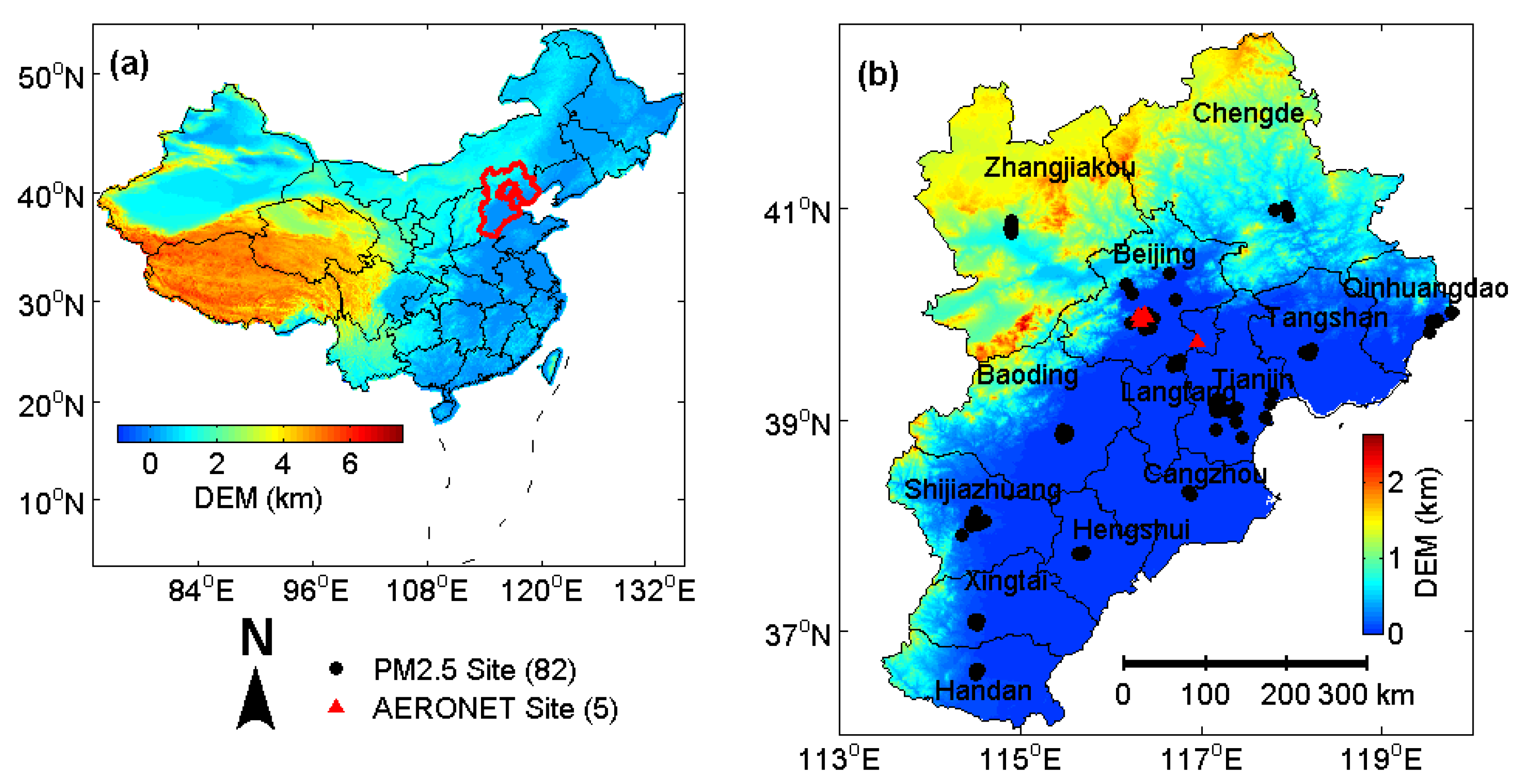
2.1. Study Area

The BTH region, also known as the Jing–Jin–Ji region, is the capital region of China. As the core area of the Bohai Economic Rim, the BTH region consists of two municipalities (Beijing and Tianjin) and 11 prefecture-level cities in Hebei Province. As shown in Figure 1, the BTH region with an area of 217,127 km² is located in northeastern mainland China between the longitudes of 113° to 120°E and latitudes of 36° to 43°N. With a temperate continental monsoon climate, the BTH region has humid and hot summers and dry and cold winters. In 2014, the annual average temperature in the BTH region was from 3.8 °C to 15.5 °C, whereas the annual average precipitation was around 400 mm. The dense population, industrialization, congested local traffic, and coal consumption of the BTH region all contributed to its status as the most concentrated PM2.5 region in China [1,18].

2.2. Datasets

The datasets used in this study included Himawari-8 Level 3 hourly AOD data and hourly observation data of surface PM2.5 concentration in the BTH region (Figure 1). Datasets covering more than a year (from July 2015 to March 2017) were used. The center of Himawari-8 is 140.7°E over equator, and the observation area is located from 80°E to 160°W and from 60°N to 60°S [28]. Himawari-8 can provide AODs at 500 nm and Ångström exponents with 10 min intervals and 5 km coverage over about one-third of the Earth (i.e., Western Pacific Ocean, East and Southeast Asia, and Oceania) [25,26]. The AODs were subjected to quality assurance with four confidence levels, namely, “very good,” “good,” “marginal,” and “no confidence” (or “no retrieval”). In this study, we only evaluated aerosol retrievals with the highest confidence level (“very good”). Himawari-8 hourly AODs with high quality were evaluated by comparing with AERONET measurements at level 1.5 because the accuracy reports of Himawari-8 retrievals were scarce. AERONET AODs could be used as a basis of comparison for satellite validation because their accuracy was less than 0.02 [29].

Hourly surface PM2.5 mass concentrations were obtained from the official website of the China Environmental Monitoring Center, which has been described in detail in a previous work [30]. Automated monitoring systems were installed in each site and used to measure the ambient concentration of SO₂, NO₂, O₃, CO, and PM2.5 and PM10 according to China Environmental Protection Standards. Meteorological data were obtained from reanalysis datasets (i.e., ERA-Interim) of the European Centre for Medium-Range Weather Forecasts (ECMWF). The ECMWF uses data assimilation systems and forecasting models to reanalyze observation datasets [31]. The ERA-Interim, one of the reanalysis datasets of ECMWF, offers a global atmosphere reanalysis since 1979. Meteorological data from the ERA-Interim include surface relative humidity (RH, %), and boundary layer height (BLH, m). The surface type is approximated by the Normalized Difference Vegetation Index (NDVI), which is obtained from MODIS 16-day NDVI production “CMG 0.05 Deg 16 days NDVI” in “MOD13C1/MYD13C1.” An NDVI larger than 0.4 usually indicates vegetated areas, whereas a smaller value refers to soil-dominated surface in generally [27]. Additionally, the DEM covering the BTH region with a resolution of 90 m produced by the National Aeronautics and Space Administration (NASA) was downloaded from the Consortium for Spatial Information (http://srtm.csi.cgiar.org/index.asp). Detailed information of the datasets applied in this study is shown in

Table 1. Summary of datasets applied in this study.

Dataset	Variable	Unit	Temporal Resolution	Spatial Resolution	Source
PM2.5	PM2.5	μg/m3	1 h	Site	CEMC
AOD	Ground AOD	Unitless	~15 min	Site	AERONET
	Satellite AOD	Unitless	1 h	0.18	Himawari-8
Meteorological Factors	RH	%	6 h	0.125°	ECMWF
	BLH	m	3 h	0.125°
Land	NDVI	Unitless	16 days	0.05°	MODIS
	DEM	m	not available	90 m	NASA

.

3. Method

3.1. Evaluation Method of the Himawari-8 AOD

Evaluation methods were applied as follows: (1) accuracy, which refers to the average difference between two datasets; (2) precision, which is the standard deviation of the difference; (3) uncertainty, which refers to root mean square deviation; (4) correlation coefficient (R), which refers to the correlation and dependence of the statistical relationships between two datasets; and (5) percentage of Himawari-8 AODs falling within the expected error (EE) range (±(0.05 + 0.15 AOD) over land), as established by MODIS (i.e., from the continuous validation of the MODIS aerosol team). The MODIS EE is a linear envelope line below and above the 1:1 line on a scatterplot, which can encompass at least 67% (about one standard deviation) of the collocations [27,32]. The MODIS uncertainty applied in this study can assess whether the high-quality Himawari-8 AOD can achieve the accuracy of MODIS. The spatiotemporal collocations between the Himawari-8 retrievals and AERONET AODs were consistent with those of other studies [27,33,34]. We averaged all of the Himawari-8 retrievals within the 20 km radius of an AERONET site to represent the satellite aerosol value. To obtain a representative Himawari-8 AOD around an AERONET site, the requirements are as follows: approximately 20% of the total Himawari-8 AODs within the 20 km radius circle centered on an AERONET site and at least two observations obtained from the AERONET within 30 min centered on the Himawari-8 measuring time. The threshold value of 20% can be found in the evaluation study of VIIRS (Visible Infrared Imaging Radiometer Suite) retrievals [35].

3.2. PM2.5 Estimated Model

The LME model with day-specific random effects for AOD was developed in [16], which can account for daily variations in the PM2.5-AOD relationship. The day-specific LME model has been widely applied in many studies because of its high accuracy [5,18,36]. The LME model is an extension of linear regression models for data that are collected and summarized in groups. The model describes the relationship between a response variable and independent variables, with coefficients that vary with respect to one or more grouping variables. The model consists of two parts: fixed effects and random effects [18]. Fixed-effects terms are the conventional linear regression part, and random effects are associated with individual experimental units drawn at random from a group (category). Random effects have prior normal distributions with mean 0 and constant variance, whereas fixed effects do not. The LME model can represent the covariance structure related to the grouping of data by associating the common random effects to observations that have the same level of a grouping variable [37].

Given that time-varying parameters, such as RH, PM2.5 vertical, and diurnal concentration profiles, and PM2.5 optical properties influence the PM2.5-AOD relationship, the statistical model allows for time variability in this relationship. If the spatial variability of these time-varying parameters is negligible, namely, the PM2.5-AOD relationship varies minimally spatially on a given time over the spatial scale, a quantitative relationship between PM2.5 concentrations and AOD values in their corresponding grid cells can be determined on a time basis [16]. Basic LME models were applied in previous studies [17,36]. We used the fitlme function of Matlab R2016b (MathWorks company), and the model structure is expressed by Model 1:

$$\begin{array}{c}\begin{array}{cc}\mathrm{PM}{2.5}_{n,m}& =[{\beta }_0+b_{0,n,m}^{hour}]+[{\beta }_1+b_{1,n,m}^{hour}]\times AO{D}_{n,m}+{\beta }_2\times R{H}_{n,m}+{\beta }_3\times BL{H}_{n,m}\hfill \\ & +{\beta }_4\times DE{M}_{n,m}+{\beta }_5\times NDV{I}_{n,m}+{\epsilon }_{n,m};\hfill \end{array}\\ (b_{0,n,m}^{hour},b_{1,n,m}^{hour})~N[(0,0,\sum )],{\epsilon }_{n,m}~N(0,{\sigma }^2);\end{array}$$

(1)

where n represents the monitoring grid index and m represents the hour (e.g., PM2.5_n,m represents the hourly average ground-level PM2.5 measurements at time m at monitoring grid n); β₀ and b_0,n,m are the fixed and random intercepts, respectively; β₁ and $b_{1,n,m}^{hour}$ are the fixed and hour-specific random slopes for AOD predictor, respectively; and β₂–β₅ are the fixed slopes for other predictors. Fixed effects correspond to the average effects of predictors on PM2.5 concentrations for the entire period. Random terms reflect the hour-to-hour variations in the AOD–PM2.5 relationship influenced by meteorology and satellite retrieval conditions. In addition, ${\epsilon }_{n,m}\sim N(0,{\sigma }^2)$ represents the observation error, and ∑ represents the variance–covariance matrix of the random effects.

The assumption of PM2.5-(AOD, predictors) relationships vary minimally spatially on a given day over a specific region, and neglect of spatial non-stationarity in regional scales is the premise for estimating PM2.5 by Equation (1) [16,18]. Therefore, one of the limitations of the aforementioned model is that it does not consider spatial variabilities in large-region regressions, which is important for estimating geographical elements in large regions. Different cities are affected by various pollution sources, meteorological conditions, population densities, number of vehicles, and so on. All these factors influence the large-region regressions of LME models. Given that our study area was relatively large and our study period was relatively long, the relationship between PM2.5 and AOD was expected to vary in both space and time. To address both the spatial and temporal heterogeneity of the PM2.5–AOD relationship, we developed an improved LME model to fit the random (including hour- and location-specific) intercepts for the whole model and the random slopes for the AODs. We consider that the hour and location have corporate effect on the large-region regression for AOD-PM2.5 relation, which can be expressed as follows (Model 2):

$$\begin{array}{c}\begin{array}{cc}\mathrm{PM}{2.5}_{n,m}& =[{\beta }_0+b_{0,n,m}^{hour*location}]+[{\beta }_1+b_{1,n,m}^{hour*location}]\times AO{D}_{n,m}+{\beta }_2\times R{H}_{n,m}\hfill \\ & +{\beta }_3\times BL{H}_{n,m}+{\beta }_4\times DE{M}_{n,m}+{\beta }_5\times NDV{I}_{n,m};\hfill \end{array}\\ (b_{0,n,m}^{hour*location},b_{1,n,m}^{hour*location})~N[(0,0,\sum )],{\epsilon }_{n,m}~N(0,{\sigma }^2);\end{array}$$

(2)

The term $hour*location$ used in the model is only the value of A times B, which represents the group-level parameters for calculating the random effects ($b_{0,n,m}^{hour*location}$ and $b_{1,n,m}^{hour*location}$). This term can be written as “$hour:location$” in Matlab. To represent a location (longitude and latitude) as a single value, we defined a complex number including location information as:

$$Location=longitude+latitude*i$$

(3)

where the real and imaginary parts of the expression correspond to longitude and latitude, respectively.

To obtain the PM2.5 estimation at a large region, $b_{0,n,m}^{hour*location}$ and $b_{1,n,m}^{hour*location}$ can be derived from the nearest location and corresponding hour training in the model. “Predict” function in Matlab can estimate predicted responses from the trained LME model at the values in the new datasets. However, the “predict” function cannot search for the nearest location for estimating PM2.5 in a new location. Therefore, we rewritten the “predict” function with the ability of search for the “nearest” PM2.5 site trained in the model. If we cannot find an appropriate random effect from a group-level in the trained model for estimating PM2.5 at a time and location, the PM2.5 in this case will be removed. As a practical technique that extends the ordinary LME model, Model 2 can examine the spatial variation at a regional scale.

In this study, the 10-fold CV was selected to compare and verify the performance of the LME and improved LME models. All of the samples were split into ten folds; that is, each fold was set approximately 10% of the total sample number. For each fold, one part was used for validation, whereas the remaining nine parts were used for training. This process was repeated for every fold. The predicted PM2.5 concentrations from all 10-fold processes were compared with the measured PM2.5 concentrations. Model performance was assessed by a determination coefficient (R²), root mean square error (RMSE), and mean absolute error (MAE).

4. Results

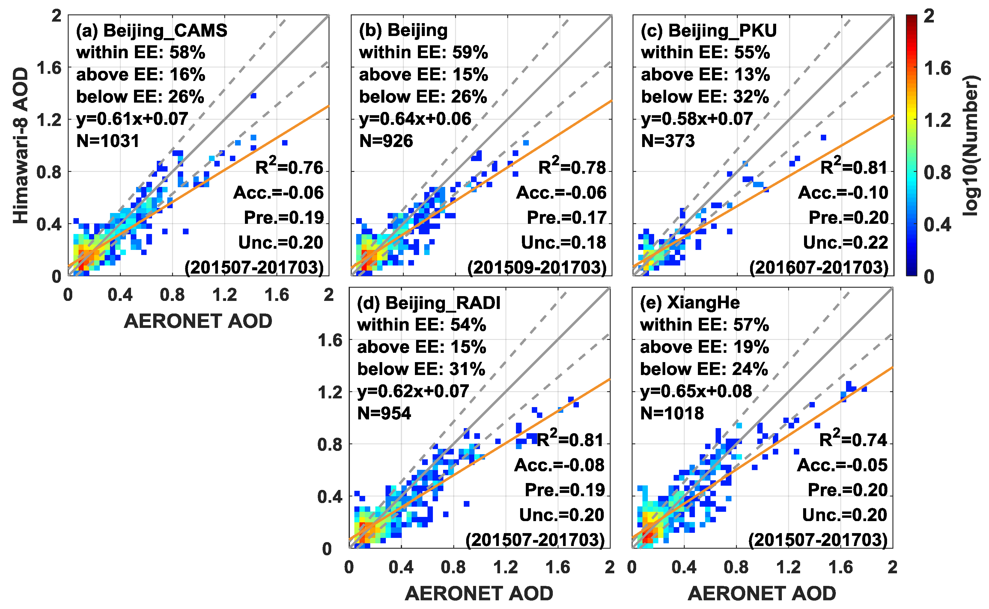
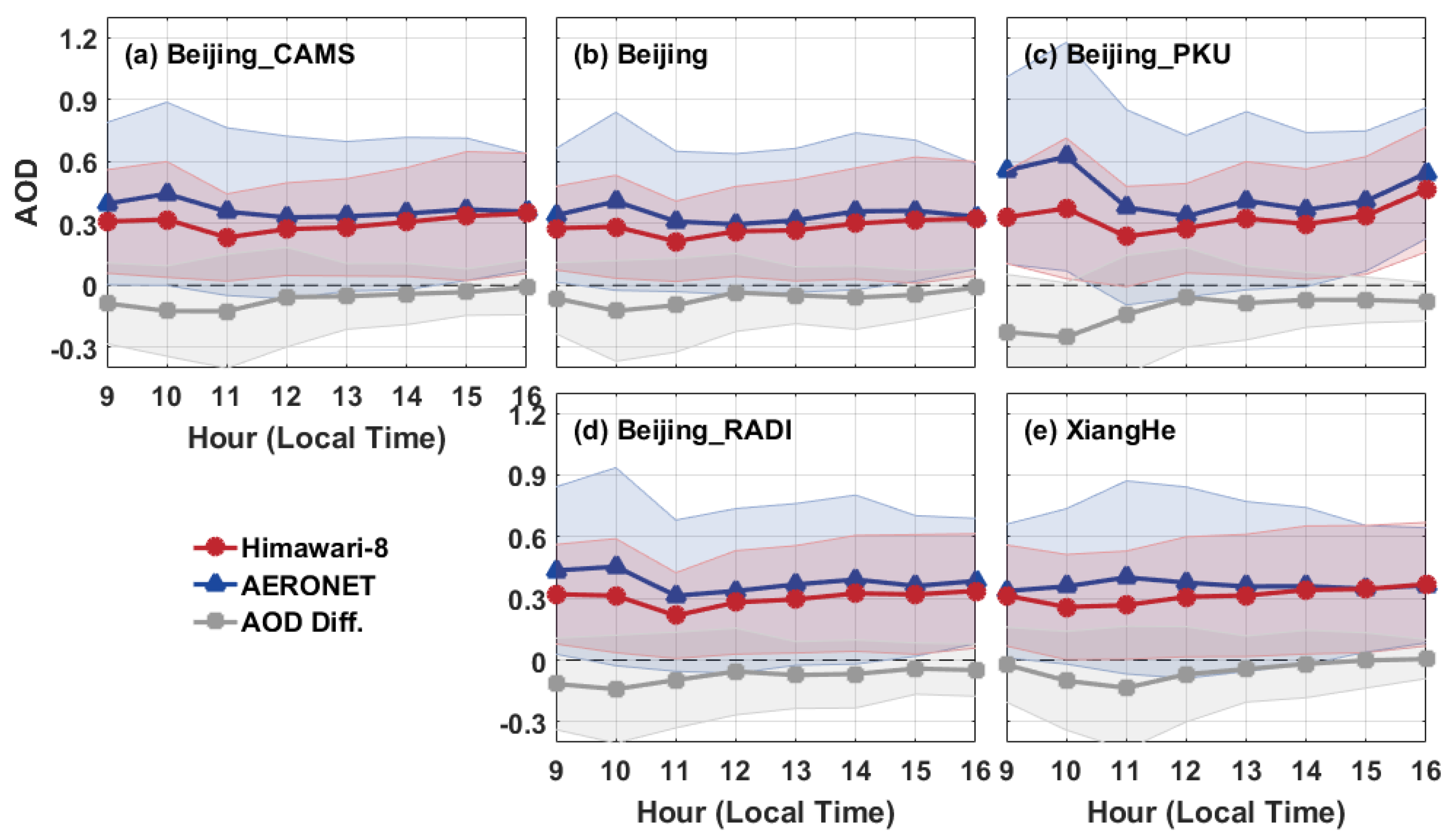
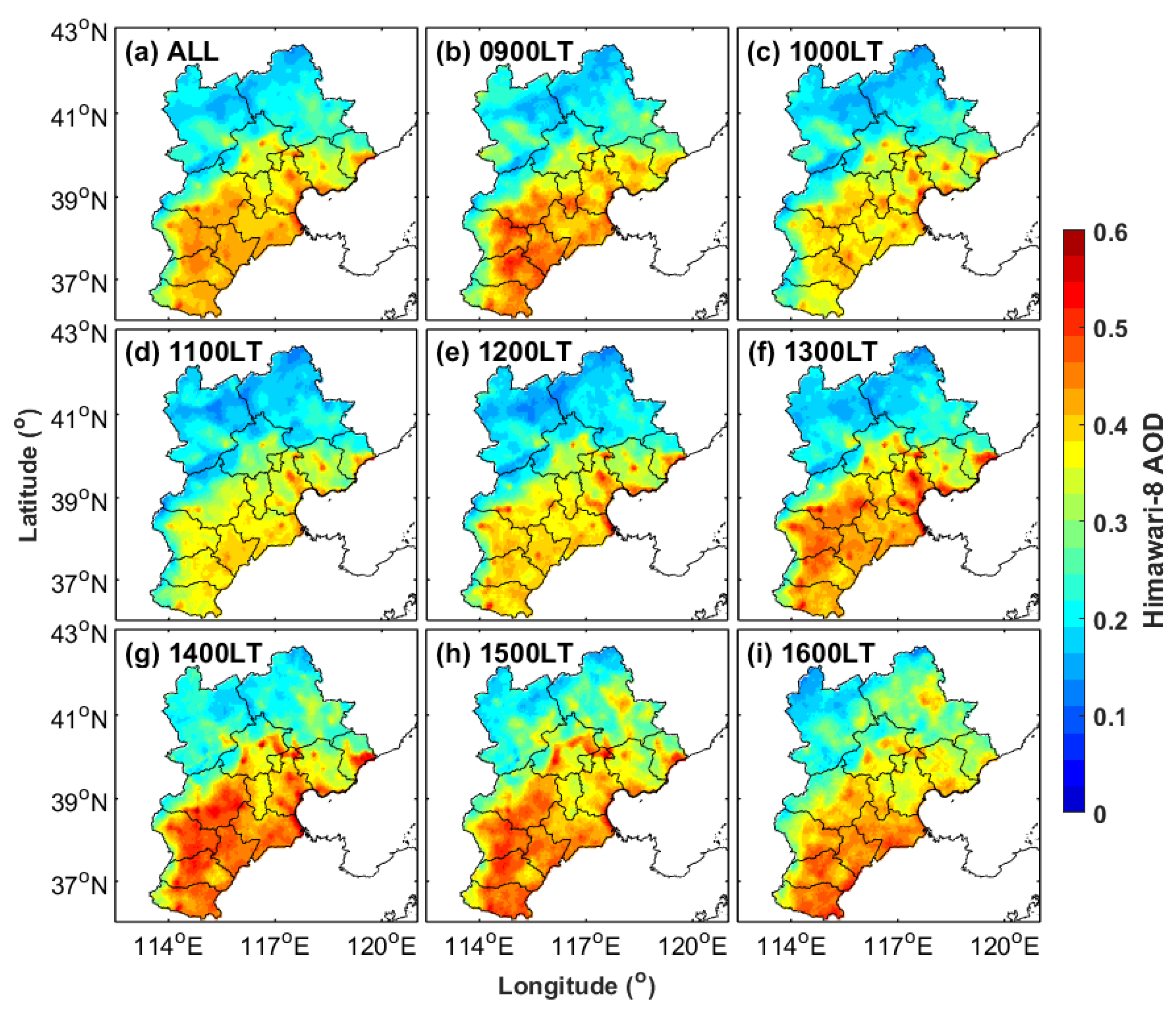
4.1. Evaluation of Himawari-8 AOD

The results of the matchup comparison between Himawari-8 and AERONET are shown in Figure 2a–e, and the corresponding statistics are listed in

Table 2. Comparative statistics of collocated Himawari-8 and AERONET AODs.

Site	N	Accuracy	Precision	Uncertainty	R2	% Above/Within/Below EE
Beijing_CAMS	1031	–0.06	0.19	0.20	0.76	16/58/26
Beijing	926	–0.06	0.17	0.18	0.78	15/59/26
Beijing_PKU	373	–0.10	0.20	0.22	0.81	13/55/32
Beijing_RADI	954	–0.08	0.19	0.20	0.81	15/54/31
XiangHe	1018	–0.05	0.20	0.20	0.74	19/57/24

. About 1000 instantaneous high-quality matchups of Himawari-8 and AERONET were determined for Beijing_CAMS, Beijing, Beijing_RADI, and Xianghe during the study period. The comparison of the Himawari-8 AODs against the AERONET observations showed the performances of Himawari-8 retrievals at the five sites, all of which exhibited high correlations (R²: 0.74–0.81), low uncertainty (0.18–0.22), and a large percentage (54–59%) of retrievals falling within the EE. Himawari-8 also showed a slight underestimation with accuracy of about −0.06. The linear regression (yellow line in Figure 2) between AERONET and Himawari-8 retrievals demonstrates the slope from 0.58 to 0.65 and the positive intercept from 0.06 to 0.08. Overall, the performances of the current Himawari-8 AOD retrievals at the five sites were almost consistent with the AERONET AODs.

The time series of the hourly Himawari-8 AODs, AERONET measurements, and AOD bias with standard deviations (shadows) during the assessment period at the five AERONET sites are shown in Figure 3. The AODs of Himawari-8 and AERONET appeared to be coincident with each other. However, an underestimation of the Himawari-8 AOD was observed from 0900 to 1100 local time (LT) in the five AERONET sites.

Figure 4 presents the spatial and hourly Himawari-8 AOD dataset at daytime from July 2015 to March 2017. The spatial distributions of the averaged AOD indicated large values in the BTH central and south regions, whereas small values emerged over the northwest region. The average AOD obtained from Himawari-8 was 0.32 ± 0.27. The average maximum AOD for the daytime was 0.38 ± 0.31 at 1500 LT. The mean AOD at 1100 LT was minimum with a mean AOD of 0.30 ± 0.26. Variations in mean AODs at the BTH region could be partially attributed to the underestimated Himawari-8 AODs from 0900 to 1200 LT (Figure 3).

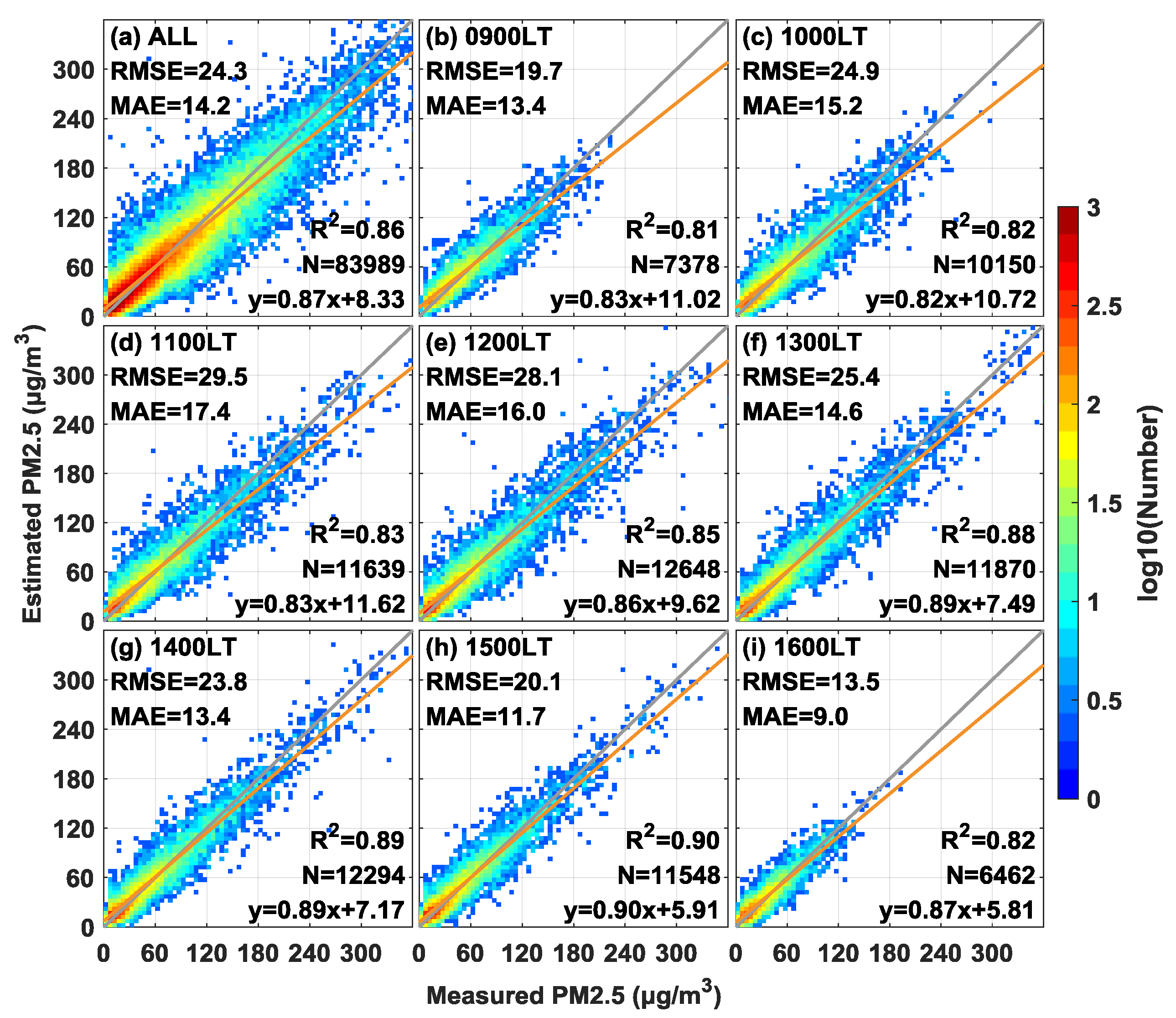
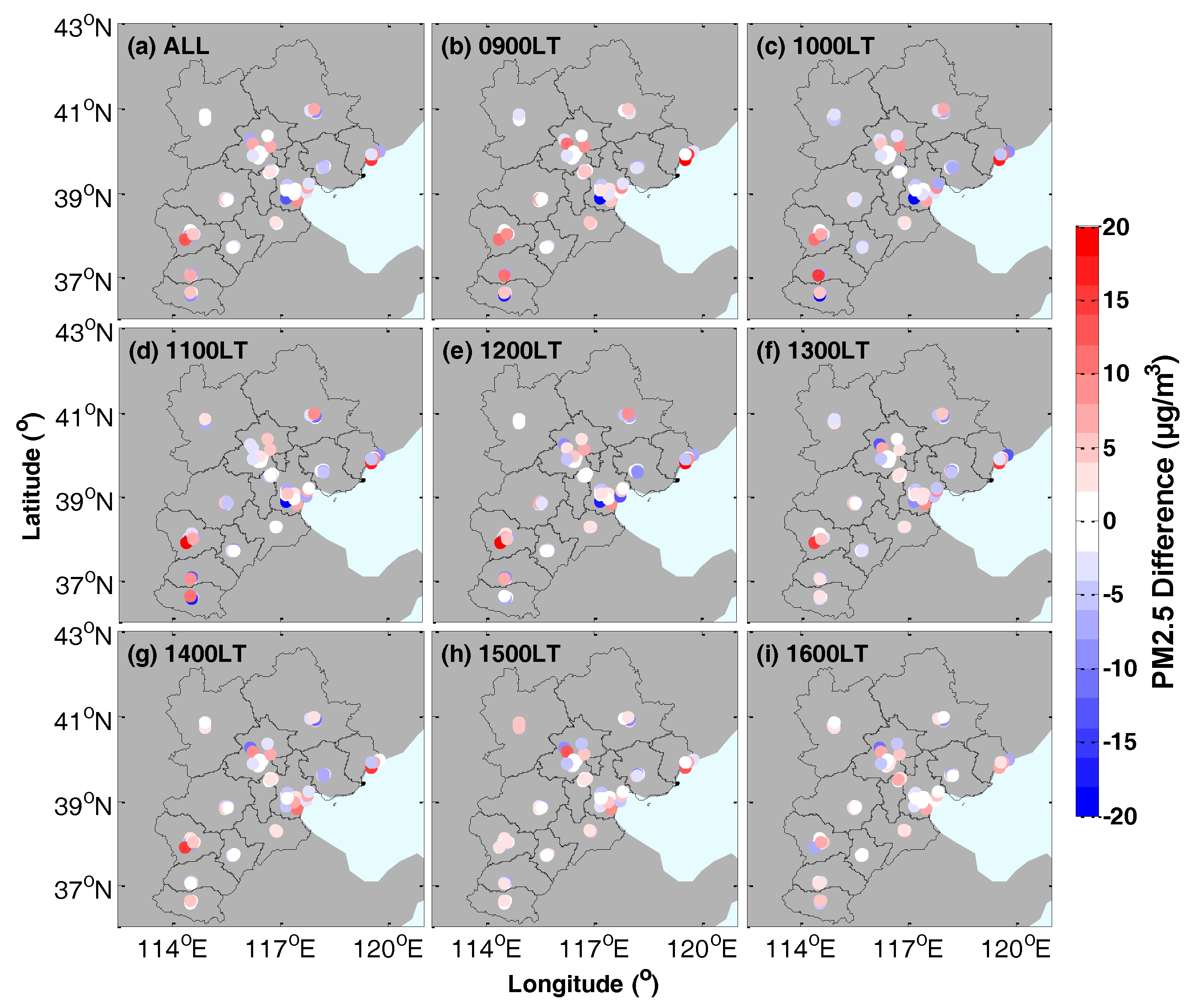
4.2. Verification of Estimated PM2.5

To train the model, ground PM2.5 and these predictors require time–space consistency. Therefore, surface PM2.5 measurements should match the Himawari-8 AODs in space and time. We averaged all Himawari-8 retrievals within the 30 min and 5 km radius of a PM2.5 monitoring site to represent the satellite AOD value. To evaluate how much the AOD, meteorological, and land parameters used in the final model could improve the model performance, we fitted different models with various predictors as shown in

Table 3. Result comparison of model fitting with different predictors.

ID	Predictor(s)	Group Variable	AIC	R2	RMSE	MAE
Test 1	AOD	Day	859,622.35	0.64	39.3	25.0
Test 2	AOD	Hour	845,625.88	0.74	33.1	20.4
Test 3	AOD; NDVI	Hour	845,589.45	0.74	33.1	20.4
Test 4	AOD; RH	Hour	845,569.14	0.74	33.1	20.4
Test 5	AOD; BLH	Hour	845,488.73	0.74	33.1	20.5
Test 6	AOD; DEM	Hour	844,323.77	0.74	32.9	20.4
Test 7	Model 1 without AOD	Hour	876,681.07	0.59	41.4	26.7
Test 8	Model 1 without $b_{0,n,m}^{hour*location}$	Hour	852,313.20	0.70	35.8	22.6
Test 9	Model 1	Hour	844,079.65	0.74	32.8	20.4
Test 10	Model 2 without AOD	Hour; location	815,754.76	0.83	26.6	15.8
Test 11	Model 2	Hour; location	809,533.48	0.93	17.1	10.1

. The Akaike information criterion (AIC) provides the relative quality of statistical models for a given dataset. The finalized LME model is generally determined based on the model performance denoted by fitting the R² (highest) and AIC (lowest) values [20]. The performances of models were assessed by coefficient of determination (R²), MAEs, and RMSEs between the measured and estimated PM2.5 concentrations. The MAE was defined as (sum of absolute errors)/(the number of observations). The RMSE was defined as the square root of the mean of the squared errors.

The LME model with day-specific random effects is widely used in PM2.5 estimation [5,17]. Tests 1 and 2 using AOD as the only independent variable (the AOD-only model) showed that the LME model with hour-specific random effects exhibited better performance than that with day-specific effects. Tests 3–6 reveal that these predictors slightly improved for the model. We also fitted a model only using meteorological and land data without AOD (the non-AOD model) to determine how AOD could benefit the model performance (Tests 7 and 10). We found that AOD had an obvious positive effect on Models 1 and 2. If the intercept without random effects (Test 8), the performance is worse than Test 9 (Model 1). A comparison of Models 1 and 2 demonstrated that the improved model exhibited outstanding performance.

Table 4. Analysis of variance (F-test and p-value) explained by each of the individual terms in different models. Beta is the coefficient of the fixed term for the two models.

Term	Model 1			Model 2
	F-Test	p-Value	Beta	F-Test	p-Value	Beta
Intercept	767.6983	<0.01	39.43	2.0496 × 103	<0.01	54.44
AOD	1.2631 × 103	<0.01	96.38	4.9156 × 103	<0.01	104.34
RH	100.7208	<0.01	−0.15	38.2626	<0.01	0.11
DEM	1.2633 × 103	<0.01	−0.03	326.3786	<0.01	−0.02
BLH	216.8013	<0.01	−0.01	1.7214 × 103	<0.01	−0.02
NDVI	2.5560	0.11	−3.06	339.0167	<0.01	−28.91

displays the analysis of variance (F-test and p-value) explained by each of the individual terms in Models 1 and 2. All p-values (<0.01) indicate significant effects of these predictors for the corresponding model. Beta is the coefficient of the fixed term for the two models.

Table 5. Standard deviations of normal distribution for the random-effects terms in the two models.

	Model 1			Model 2
	${\mathit{b}}_{0,\mathit{m}}^{\mathit{hour}}$	${\mathit{b}}_{1,\mathit{m}}^{\mathit{hour}}$	${\mathit{\epsilon }}_{\mathit{n},\mathit{m}}$	${\mathit{b}}_{0,\mathit{m}}^{\mathit{hour}*\mathit{location}}$	${\mathit{b}}_{1,\mathit{m}}^{\mathit{hour}*\mathit{location}}$	${\mathit{\epsilon }}_{\mathit{n},\mathit{m}}$
Estimate	37.03	124.64	33.76	41.02	112.90	19.84
Lower	35.68	120.39	33.59	39.97	109.81	19.72
Upper	38.42	129.04	33.92	42.09	116.08	19.95

displays the estimate for the standard deviation of normal distribution for the random-effects term for intercept, AOD, and error grouped by hour for each day. Their confidence interval is small, which indicates that the random effects for intercept, AOD, and error grouped by hour for each day and $b_{1,m}^{hour*location}$ is significant.

Previous studies on the PM2.5–AOD statistical model mainly used the site-based CV [16] and sample-based 10-fold CV methods [2]. For the site-based CV, one of the PM2.5 monitoring sites was used for validation, and the rest of the sites were used for model fitting; this process was conducted for each round of validation. In this section, the two CVs were selected to verify the performance of the proposed model. A comparison of the performance of the LME and improved LME models is presented in

Table 6. Result comparison of model fitting and cross-validation for Model 1 and 2.

Model	N	Site Cross-Validation			10-Fold Cross-Validation
		R2	RMSE	MAE	R2	RMSE	MAE
Model 1	83,989	0.73	34.4	21.7	0.73	34.5	21.7
Model 2	83,989	0.87	24.1	14.0	0.86	24.5	14.2

.

The predictive performances of the LME models during the study period were low with R² of 0.73 and 0.73, RMSE of 34.4 µg/m³ and 34.5 µg/m³, and MAE 21.7 µg/m³ and 21.7 µg/m³ for site-based CV and 10-fold CV, respectively. The superiority of the improved model to the LME model in estimating PM2.5 concentrations was confirmed by the site-based CVs and the 10-fold CVs, as evidenced by the RMSE and MAE values (Table 6). Site-based CVs could verify the performance of the improved LME model on location without any PM2.5 measurements. The 10-fold CV for the improved LME model presented higher R² (0.86 versus 0.73), lower RMSE (24.5 µg/m³ versus 34.5 µg/m³), and lower MAE (14.2 µg/m³ versus 21.7 µg/m³) compared with the ordinary LME model. Zheng et al. [18] used LME models to estimate daily PM2.5 concentrations in the BTH region with a R² of 0.77 in the 10-fold CV (predictor: MODIS AODs, meteorological factors, and tropospheric NO₂). Therefore, to ensure a relatively good estimation of PM2.5 concentrations, the improved LME model (Model 2) was applied in our study analysis.

Figure 5 presents the scatterplot of the comparison between measured and estimated PM2.5 concentrations in the BTH region at different hours. In these scatterplots, colors indicate the number of data points for a corresponding pixel. The high CV R² values of the improved LME model (i.e., 0.86 for all data and 0.81–0.90 for different hours) prove the acceptable performance of the model in the BTH region; that is, the model yielded reasonable predictions. However, the different CV R² values at different hours (e.g., maximum of 0.90 at 1500 LT; minimum of 0.81 at 0900 LT) imply that the performance of the improved LME model was higher at noon and in the afternoon than for the other hours during daytime. Figure 3 presents the underestimations of the Himawari-8 AODs from 0900 to 1100 LT at the five AERONET sites. Discrepancies in hourly results such as for the CV RMSE at 1600 LT (13.4 μg/m³), which was smaller than for the other hours (above 20 μg/m³), could be attributed to the relatively small number of matchups. Furthermore, the MAE in the BTH region was 14.2 μg/m³ for all matchups, and the values ranged from 9.0 μg/m³ to 17.4 μg/m³ for the different hours. PM2.5 difference was equal to the estimated value minus the measured PM2.5 (

Table 7. Averages of estimated and measured PM2.5 at different hours.

Local Time	N	R2	Estimated PM2.5	Measured PM2.5	PM2.5 Bias
ALL	83,989	0.86	61.6 ± 61.4	61.5 ± 65.8	0.1 ± 24.3
0900	7378	0.81	58.6 ± 41.5	57.6 ± 45.2	1.1 ± 19.7
1000	10,150	0.82	63.5 ± 53.2	64.5 ± 58.9	–1.0 ± 24.9
1100	11,639	0.83	71.0 ± 65.2	71.7 ± 71.8	–0.8 ± 29.5
1200	12,648	0.85	66.9 ± 67.1	67.0 ± 72.3	–0.1 ± 28.1
1300	11,870	0.88	66.7 ± 69.6	66.6 ± 73.4	0.1 ± 25.4
1400	12,294	0.89	62.9 ± 67.5	62.3 ± 71.0	0.6 ± 23.8
1500	11,548	0.90	54.8 ± 60.6	54.1 ± 63.8	0.6 ± 20.1
1600	6462	0.82	35.3 ± 30.3	34.0 ± 31.7	1.3 ± 13.4

).

Figure 6 shows the spatial distributions of the estimated PM2.5 errors in individual PM sites in the BTH region, which could be used to evaluate the accuracy of the improved LME model for each PM2.5 monitoring site. The red (blue) solid circles indicate that the estimated PM2.5 was overestimated (underestimated). Figure 6a shows the mean bias from all available data. Accordingly, the PM2.5 concentrations were overestimated in one of the sites in Qinghuangdao (~20 μg/m³) and Shijiazhuang (~15 μg/m³). Coasts with complex surfaces and aerosol types may reduce the performance of the Himawari-8 aerosol retrievals. In Qinghuangdao, the sites near the coast may result in overestimation at all hours. By contrast, sites with underestimations were observed in some parts of Tianjing. As shown in Figure 6, the rest of the sites displayed light-colored solid circles, which indicated unclear estimated biases. Despite the general consistency between estimated and measured PM2.5 concentrations in Figure 6a, site discrepancies were obvious in different hours, as shown in Figure 6b–i. In the ante meridiem (0900–1100 LT), most of the mild positive biases were observed in Beijing, Shijiazhuang, and Xingtai, whereas negative biases existed in Tianjing and Handan. The Himawari-8 AODs, which were highly accurate at noontime, might have contributed to the slight biases at 1200–1500 LT.

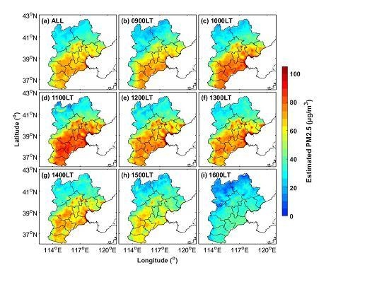
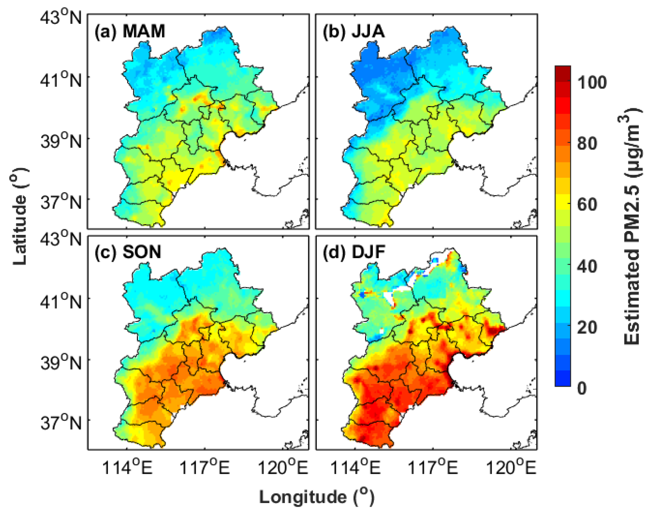
4.3. Spatial Distribution of PM2.5

The hourly spatial distributions of PM2.5 in the BTH region (Figure 7) were spatially heterogeneous, which implies the applicability of the improved LME model. Many fine-scale variations in AOD of Figure 4 show up as variations in the PM2.5 estimates in Figure 7. The consistency of spatial distribution between AOD and PM2.5 indicate the geographic correlations of AOD and PM2.5.

Urban areas with high PM2.5 concentrations, such as Beijing, Shijiazhuang, Xingtai, and Handan, were effectively captured by the improved LME model. The average PM2.5 in the BTH region was 58.2 ± 52.7 μg/m³ (Table 8), which exceeded the World Health Organization Air Quality Interim Target-1 standard of 35 μg/m³. The average PM2.5 in southern BTH was larger than 50 μg/m³, which was considerably higher than those in the northern regions. Severely-polluted areas were located in Cangzhou and Hengshui, as evidenced by the large mean PM2.5 concentrations of 66.9 + 58.7 and 67.8 + 56.7 μg/m³, respectively. Industrial production and high vehicle population contributed to high anthropogenic emissions, further resulting in a relatively high PM2.5 in southern BTH. Low PM2.5 in northern BTH (i.e., Zhangjiakou and Chengde) were observed at less than 35 μg/m³ on average; these areas have hilly topography and low human activities, resulting in low anthropogenic emissions. Our results were similar to that of a previous study [8], which reported an annual mean PM2.5 concentration of 45–55 μg/m³ in the southern anthropogenic area. The satellite-derived population-weighted average of PM2.5 in Beijing was 51.2 μg/m³ during the study period (March 2013 to April 2014) [17]. A one-year study on the PM2.5 estimations in the BTH region using a generalized additive model presented an annual mean value of 69.4 µg/m³ with values ranging from 13.3 µg/m³ to 133.7 µg/m³ [9].

The spatial distributions of the hourly PM2.5 estimations differed across hours (Figure 7b–i); that is, 1100 LT was most polluted with a large mean PM2.5 of 65.5 ± 54.6 μg/m³ (

Table 8. Average Himawari-8 AOD and estimated PM2.5 at different hours in the BTH region.

Local Time	Himawari-8 AOD	Estimated PM2.5 (μg/m3)
ALL	0.32 ± 0.27	58.2 ± 52.7
0900	0.33 ± 0.25	52.6 ± 38.0
1000	0.31 ± 0.26	59.7 ± 47.6
1100	0.30 ± 0.26	65.5 ± 54.6
1200	0.32 ± 0.27	61.3 ± 56.8
1300	0.34 ± 0.28	62.2 ± 59.9
1400	0.37 ± 0.30	59.5 ± 58.1
1500	0.38 ± 0.31	52.3 ± 50.9
1600	0.37 ± 0.29	35.2 ± 26.9
MAM	0.30 ± 0.26	46.0 ± 38.4
JJA	0.38 ± 0.32	42.5 ± 29.8
SON	0.36 ± 0.31	57.8 ± 50.7
DJF	0.26 ± 0.23	71.5 ± 70.1

), as opposed to the minimum average of PM2.5 at 1600 LT. The hourly variations were consistent with the measured mean PM2.5 values (Table 7), but these mean values were smaller because the estimated PM2.5 concentrations were averaged using datasets from urban and suburban regions. The variations in hourly Himawari-8 AODs also disagreed with the estimated PM2.5; for example, the maximum PM2.5 (65.5 ± 54.6 μg/m³) corresponded to the minimal AOD (0.30 ± 0.26) at 1100 LT. Several factors might have influenced the variations, such as meteorological factors, which could synergistically affect PM2.5 concentrations.

The spatial and seasonal images of averaged PM2.5 estimations obtained from the improved LME model are shown in Figure 8. The different seasons in Figure 8 are denoted as MAM (March, April, and May), JJA (June, July, and August), SON (September, October, and November), and DJF (December, January, and February). The void regions in northern regions in winter were due to the limitation of Himawari-8 in retrieving high-quality AOD under scarce vegetation in winter. Strong seasonality of PM2.5 concentrations was also found from the averaged PM2.5 concentration. Winter was the most polluted season with a mean estimated PM2.5 of 71.5 ± 70.1 µg/m³, whereas summer was the cleanest season with a mean predicted concentration of 42.5 ± 29.8 µg/m³. The mean predicted PM2.5 concentration was 46.0 ± 38.4 µg/m³ in spring and 57.8 ± 50.7 µg/m³ in autumn.

5. Discussion

Given the sparse distribution of stationary PM2.5 sites, satellite data with wide spatial coverage are growing as one of the most important supplementary tools to estimate PM2.5 concentrations in a wide geographical space. The relationship between surface PM2.5 and column-integrated AOD is associated with vertical and size distribution of aerosols [38,39]. The particulate matter vertical distribution has been considered from a physics perspective, which could improve the correlation between PM2.5 and AOD [40,41]. Humidity correction for PM2.5 estimation is necessary because “dry” PM2.5 measurements after particles are heated to 50 °C may undervalue the aerosol particle mass (aerosol hygroscopicity results in AOD being affected by humidity) [42].

In this study, related factors, such as AOD, meteorological parameters, and land type, are individually integrated into the typical LME model to test their benefits on model performance. BLH and RH can be regarded as the correction factors of height and humidity, respectively [39]. Moreover, this study developed an improved LME model for satellite-based PM2.5 estimation. The improved LME model considered the spatial and temporal heterogeneity of the PM2.5–AOD relationship. As expected, the improved LME model clearly showed better performance in estimating PM2.5 concentrations from Himawari-8 AOD compared with the typical LME model in the BTH region. This result confirmed the necessity of the LME model in simultaneously considering spatial–temporal heterogeneity for PM2.5-(AOD, predictors) relationships.

The differences in performance of the improved model at 0900 and 1100 LT might be due to the underestimation of the Himawari-8 AODs at the specified times. PM2.5 underestimations predominantly occurred when the measured ground-level PM2.5 concentrations were high (i.e., greater than 80 μg/m³). Meanwhile, overestimated PM2.5 concentrations existed with slightly polluted levels, which was similar to those in the same region according to another study [18]. This result could be attributed to the nonlinear relationship between PM2.5 concentrations and AODs at different aerosol loadings [9]. Moreover, the predicted PM2.5 concentrations using the average AOD for the PM2.5 monitoring sites within the 5 km radius may not fully represent the site measurements.

For the hourly spatial distributions of PM2.5 in the BTH in Figure 7i, estimated PM2.5 at LT 16:00 showed a significant decrease. The Himawari-8 retrievals with high quality at 1600LT in winter were less than that in summer because the sun angle was probably too low for Himawari-8 retrievals at 1600LT in winter. The PM2.5 concentration in summer was lower than that in winter (Figure 8). Therefore, the limited collocations between ground PM2.5 and satellite-based AODs may result in the decrease at LT 16:00.

6. Conclusions

The spatial distributions of hourly PM2.5 concentrations are significant and necessary in understanding PM2.5 evolution. In this study, the primary estimation of hourly PM2.5 concentrations at daytime in the BTH region was executed with a proposed improved LME model using ground-based PM2.5 observations and collocated Himawari-8 (Level 3) with hourly AODs from July 2015 to March 2017.

(1) The Himawari-8 AOD with a “very good” confidence level was evaluated by comparing its values with the AERONET observations for the given study period. The Himawari-8 AODs at the five AERONET sites presented mild underestimations of about −0.06 with 57% of the AODs falling within the EE made from MODIS [±(0.05 + 0.15 AOD)].

(2) An improved LME model was developed for hourly PM2.5 estimation based on the relation between PM2.5 and AOD. The estimated PM2.5 concentrations agreed well with the surface PM2.5 measurements, as evidenced by the high R² (0.86) and low RMSE (24.5 μg/m³) based on 10-fold cross-validation.

(3) The average PM2.5 estimations of the improved LME model in the southern BTH were higher than those in the northern regions. The average PM2.5 concentration in the BTH region was 58.2 ± 52.7 μg/m³. The estimated hourly PM2.5 concentrations ranged extensively from 35.2 ± 26.9 μg/m³ (1600 LT) to 65.5 ± 54.6 μg/m³ (1100 LT).

Future studies can focus on the improvement of the LME model to depict the spatial distributions of PM2.5 concentrations using fine spatial resolutions. The accurate derivation of surface PM2.5 concentrations from satellite retrievals largely depends on the quality of satellite aerosol products. Thus, efforts to improve the Himawari-8 AODs for hourly PM2.5 estimation or observation should be considered.

References

1. Ma, X.; Wang, J.; Yu, F.; Jia, H.; Hu, Y. Can MODIS AOD be employed to derive PM2.5 in Beijing-Tianjin-Hebei over China? Atmos. Res. 2016, 181, 250–256. [Google Scholar] [CrossRef]
2. Zhang, T.; Gong, W.; Wang, W.; Ji, Y.; Zhu, Z.; Huang, Y. Ground level PM2.5 estimates over China using satellite-based geographically weighted regression (GWR) models are improved by including NO2 and enhanced vegetation index (EVI). Int. J. Environ. Res. Public Health 2016, 13, 1215. [Google Scholar] [CrossRef] [PubMed]
3. Pope, C.A. Epidemiology of fine particulate air pollution and human health: biologic mechanisms and who’s at risk? Environ. Health Perspect. 2000, 108, 713–723. [Google Scholar] [CrossRef] [PubMed]
4. Zhang, Y.-L.; Cao, F. Fine particulate matter (PM2.5) in China at a city level. Sci. Rep. 2015, 5. [Google Scholar] [CrossRef] [PubMed]
5. Lee, H.J.; Chatfield, R.B.; Strawa, A.W. Enhancing the applicability of satellite remote sensing for PM2.5 estimation using MODIS deep blue AOD and land use regression in California, United States. Environ. Sci. Technol. 2016, 50, 6546–6555. [Google Scholar] [CrossRef] [PubMed]
6. Wang, W.; Gong, W.; Mao, F.; Zhang, J. Long-term measurement for low-tropospheric water vapor and aerosol by Raman lidar in Wuhan. Atmosphere 2015, 6, 521–533. [Google Scholar] [CrossRef]
7. Koelemeijer, R.B.A.; Homan, C.D.; Matthijsen, J. Comparison of spatial and temporal variations of aerosol optical thickness and particulate matter over Europe. Atmos. Environ. 2006, 40, 5304–5315. [Google Scholar] [CrossRef]
8. Xin, J.; Zhang, Q.; Wang, L.; Gong, C.; Wang, Y.; Liu, Z.; Gao, W. The empirical relationship between the PM2.5 concentration and aerosol optical depth over the background of north China from 2009 to 2011. Atmos. Res. 2014, 138, 179–188. [Google Scholar] [CrossRef]
9. Zou, B.; Chen, J.; Zhai, L.; Fang, X.; Zheng, Z. Satellite based mapping of ground PM2.5 concentration using generalized additive modeling. Remote Sens. 2017, 9, 1. [Google Scholar] [CrossRef]
10. Chu, D.A.; Kaufman, Y.J.; Zibordi, G.; Chern, J.D.; Mao, J.; Li, C.; Holben, B.N. Global monitoring of air pollution over land from the earth observing system-terra moderate resolution imaging spectroradiometer (MODIS). J. Geophys. Res. Atmos. 2003, 108. [Google Scholar] [CrossRef]
11. Gupta, P.; Christopher, S.A. Particulate matter air quality assessment using integrated surface, satellite, and meteorological products: Multiple regression approach. J. Geophys. Res. Atmos. 2009, 114. [Google Scholar] [CrossRef]
12. Liu, Y.; Sarnat, J.A.; Kilaru, V.; Jacob, D.J.; Koutrakis, P. Estimating ground-level PM2.5 in the Eastern United States using satellite remote sensing. Environ. Sci. Technol. 2005, 39, 3269–3278. [Google Scholar] [CrossRef] [PubMed] [Green Version]
13. Chen, Q.-X.; Yuan, Y.; Huang, X.; Jiang, Y.-Q.; Tan, H.-P. Estimation of surface-level PM2.5 concentration using aerosol optical thickness through aerosol type analysis method. Atmos. Environ. 2017, 159, 26–33. [Google Scholar] [CrossRef]
14. Guo, J.; Xia, F.; Zhang, Y.; Liu, H.; Li, J.; Lou, M.; He, J.; Yan, Y.; Wang, F.; Min, M.; et al. Impact of diurnal variability and meteorological factors on the PM2.5-AOD relationship: Implications for PM2.5 remote sensing. Environ. Pollut. 2017, 221, 94–104. [Google Scholar] [CrossRef] [PubMed]
15. Stafoggia, M.; Schwartz, J.; Badaloni, C.; Bellander, T.; Alessandrini, E.; Cattani, G.; de’ Donato, F.; Gaeta, A.; Leone, G.; Lyapustin, A.; et al. Estimation of daily PM10 concentrations in Italy (2006–2012) using finely resolved satellite data, land use variables and meteorology. Environ. Int. 2017, 99, 234–244. [Google Scholar] [CrossRef] [PubMed]
16. Lee, H.J.; Liu, Y.; Coull, B.A.; Schwartz, J.; Koutrakis, P. A novel calibration approach of MODIS AOD data to predict PM2.5 concentrations. Atmos. Chem. Phys. Discuss. 2011. [Google Scholar] [CrossRef]
17. Xie, Y.; Wang, Y.; Zhang, K.; Dong, W.; Lv, B.; Bai, Y. Daily estimation of ground-level PM2.5 concentrations over Beijing using 3 km resolution MODIS AOD. Environ. Sci. Technol. 2015, 49, 12280–12288. [Google Scholar] [CrossRef] [PubMed]
18. Zheng, Y.; Zhang, Q.; Liu, Y.; Geng, G.; He, K. Estimating ground-level PM2.5 concentrations over three megalopolises in China using satellite-derived aerosol optical depth measurements. Atmos. Environ. 2016, 124 Pt B, 232–242. [Google Scholar] [CrossRef]
19. Li, C.; Hsu, N.C.; Tsay, S.-C. A study on the potential applications of satellite data in air quality monitoring and forecasting. Atmos. Environ. 2011, 45, 3663–3675. [Google Scholar] [CrossRef]
20. Zou, B.; Pu, Q.; Bilal, M.; Weng, Q.; Zhai, L.; Nichol, J.E. High-resolution satellite mapping of fine particulates based on geographically weighted regression. IEEE Geosci. Remote Sens. Lett. 2016, 13, 495–499. [Google Scholar] [CrossRef]
21. Remer, L.A.; Kaufman, Y.; Tanré, D.; Mattoo, S.; Chu, D.; Martins, J.; Li, R.-R.; Ichoku, C.; Levy, R.; Kleidman, R. The MODIS aerosol algorithm, products, and validation. J. Atmos. Sci. 2005, 62, 947–973. [Google Scholar] [CrossRef]
22. Wang, W.; Mao, F.; Pan, Z.; Du, L.; Gong, W. Validation of VIIRS AOD through a comparison with a sun photometer and MODIS AODS over Wuhan. Remote Sens. 2017, 9, 403. [Google Scholar] [CrossRef]
23. Emili, E.; Popp, C.; Petitta, M.; Riffler, M.; Wunderle, S.; Zebisch, M. PM10 remote sensing from geostationary SEVIRI and polar-orbiting MODIS sensors over the complex terrain of the European Alpine region. Remote Sens. Environ. 2010, 114, 2485–2499. [Google Scholar] [CrossRef]
24. Bessho, K.; Date, K.; Hayashi, M.; Ikeda, A.; Imai, T.; Inoue, H.; Kumagai, Y.; Miyakawa, T.; Murata, H.; Ohno, T.; et al. An introduction to Himawari-8/9—Japan’s new-generation geostationary meteorological satellites. J. Meteorol. Soc. Jpn. Ser. II 2016, 94, 151–183. [Google Scholar] [CrossRef]
25. Yumimoto, K.; Nagao, T.M.; Kikuchi, M.; Sekiyama, T.T.; Murakami, H.; Tanaka, T.Y.; Ogi, A.; Irie, H.; Khatri, P.; Okumura, H.; et al. Aerosol data assimilation using data from Himawari-8, a next-generation geostationary meteorological satellite. Geophys. Res. Lett. 2016, 43, 5886–5894. [Google Scholar] [CrossRef]
26. Shang, H.; Chen, L.; Letu, H.; Zhao, M.; Li, S.; Bao, S. Development of a daytime cloud and haze detection algorithm for Himawari-8 satellite measurements over central and eastern China. J. Geophys. Res. Atmos. 2017. [Google Scholar] [CrossRef]
27. Liu, H.; Remer, L.A.; Huang, J.; Huang, H.-C.; Kondragunta, S.; Laszlo, I.; Oo, M.; Jackson, J.M. Preliminary evaluation of S-NPP VIIRS aerosol optical thickness. J. Geophys. Res. Atmos. 2014, 119, 3942–3962. [Google Scholar] [CrossRef]
28. Kurihara, Y.; Murakami, H.; Kachi, M. Sea surface temperature from the new Japanese geostationary meteorological Himawari-8 satellite. Geophys. Res. Lett. 2016, 43, 1234–1240. [Google Scholar] [CrossRef]
29. Dubovik, O.; Smirnov, A.; Holben, B.N.; King, M.D.; Kaufman, Y.J.; Eck, T.F.; Slutsker, I. Accuracy assessments of aerosol optical properties retrieved from aerosol robotic network (AERONET) sun and sky radiance measurements. J. Geophys. Res. Atmos. 2000, 105, 9791–9806. [Google Scholar] [CrossRef]
30. Xu, J.W.; Martin, R.V.; van Donkelaar, A.; Kim, J.; Choi, M.; Zhang, Q.; Geng, G.; Liu, Y.; Ma, Z.; Huang, L.; et al. Estimating ground-level PM2.5 in Eastern China using aerosol optical depth determined from the goci satellite instrument. Atmos. Chem. Phys. 2015, 15, 13133–13144. [Google Scholar] [CrossRef]
31. Molteni, F.; Buizza, R.; Palmer, T.N.; Petroliagis, T. The ECMWF ensemble prediction system: Methodology and validation. Q. J. R. Meteorol. Soc. 1996, 122, 73–119. [Google Scholar] [CrossRef]
32. Levy, R.C.; Mattoo, S.; Munchak, L.A.; Remer, L.A.; Sayer, A.M.; Patadia, F.; Hsu, N.C. The collection 6 MODIS aerosol products over land and ocean. Atmos. Meas. Tech. 2013, 6, 2989–3034. [Google Scholar] [CrossRef]
33. Xiao, Q.; Zhang, H.; Choi, M.; Li, S.; Kondragunta, S.; Kim, J.; Holben, B.; Levy, R.C.; Liu, Y. Evaluation of VIIRS, GOCI, and MODIS collection 6 aod retrievals against ground sunphotometer observations over east Asia. Atmos. Chem. Phys. 2016, 16, 20709–20741. [Google Scholar] [CrossRef]
34. Nichol, J.; Bilal, M. Validation of MODIS 3 km resolution aerosol optical depth retrievals over Asia. Remote Sens. 2016, 8, 328. [Google Scholar] [CrossRef]
35. Huang, J.; Kondragunta, S.; Laszlo, I.; Liu, H.; Remer, L.A.; Zhang, H.; Superczynski, S.; Ciren, P.; Holben, B.N.; Petrenko, M. Validation and expected error estimation of Suomi-NPP VIIRS aerosol optical thickness and angström exponent with aeronet. J. Geophys. Res. Atmos. 2016, 121, 7139–7160. [Google Scholar] [CrossRef]
36. Ma, Z.; Liu, Y.; Zhao, Q.; Liu, M.; Zhou, Y.; Bi, J. Satellite-derived high resolution PM2.5 concentrations in Yangtze River delta region of China using improved linear mixed effects model. Atmos. Environ. 2016, 133, 156–164. [Google Scholar] [CrossRef]
37. Pinheiro, J.C.; Bates, D.M. Mixed-Effects Models in S and S-PLUS; Springer: Berlin/Heidelberg, Germany, 2004. [Google Scholar]
38. Li, S.; Joseph, E.; Min, Q. Remote sensing of ground-level PM2.5 combining AOD and backscattering profile. Remote Sens. Environ. 2016, 183, 120–128. [Google Scholar] [CrossRef]
39. Zhang, Y.; Li, Z. Remote sensing of atmospheric fine particulate matter (PM2.5) mass concentration near the ground from satellite observation. Remote Sens. Environ. 2015, 160, 252–262. [Google Scholar] [CrossRef]
40. Chu, D.A.; Ferrare, R.; Szykman, J.; Lewis, J.; Scarino, A.; Hains, J.; Burton, S.; Chen, G.; Tsai, T.; Hostetler, C.; et al. Regional characteristics of the relationship between columnar aod and surface PM2.5: Application of lidar aerosol extinction profiles over Baltimore–Washington corridor during discover-AQ. Atmos. Environ. 2015, 101, 338–349. [Google Scholar] [CrossRef]
41. Barnaba, F.; Putaud, J.P.; Gruening, C.; dell’Acqua, A.; Dos Santos, S. Annual cycle in co-located in situ, total-column, and height-resolved aerosol observations in the Po Valley (Italy): Implications for ground-level particulate matter mass concentration estimation from remote sensing. J. Geophys. Res. Atmos. 2010, 115. [Google Scholar] [CrossRef]
42. Song, W.; Jia, H.; Huang, J.; Zhang, Y. A satellite-based geographically weighted regression model for regional PM2.5 estimation over the Pearl river delta region in China. Remote Sens. Environ. 2014, 154, 1–7. [Google Scholar] [CrossRef]
Figure 1. Elevation map of (a) China and (b) Beijing–Tianjin–Hebei region. (b) Spatial distributions of fine particulate matter (PM) and AERONET sites in Beijing–Tianjin–Hebei region.
Remotesensing 09 00858 g001
Figure 2. Collocations scatterplots of Himawari-8 and AERONET AODs at five sites of (a) Beijing_CAMS; (b) Beijing; (c) Beijing_PKU; (d) Beijing_RADI; and (e) Xianghe. The study period is from July 2015 to March 2017. The width of each pixel is 0.04 AOD, and the number of collocations falling within/above/below EE are represented in each figure. The yellow line is the regression line, the gray solid line is the 1:1 line, and the gray dashed lines are the expected errors (EE) envelopes.
Remotesensing 09 00858 g002
Figure 3. Time series of hourly AODs of Himawari-8 and AERONET, and hourly AOD difference between Himawari-8 and AERONET from the collocated matchups and standard deviations (shadows) over (a) Beijing_CAMS; (b) Beijing; (c) Beijing_PKU; (d) Beijing_RADI; and (e) Xianghe. The study period is from July 2015 to March 2017.
Remotesensing 09 00858 g003
Figure 4. Spatial distributions of the averaged AOD derived from the Himawari-8 for all available data (a) and different hours (0900–1600 local time) (bi). The study period is from July 2015 to March 2017.
Remotesensing 09 00858 g004
Figure 5. 10-fold cross-validation of estimated PM2.5 concentrations by comparing measured PM2.5 from all available data (a) and in different hours (0900–1600 local time) (bi). The number of samplings (N), correlation coefficients (R), and linear regressions are included in the plot.
Remotesensing 09 00858 g005
Figure 6. Differences in estimated and measured PM2.5 for individual PM monitoring sites: (a) all available data; (bi) different hours (0900–1600 local time).
Remotesensing 09 00858 g006
Figure 7. Spatial distribution of averaged PM2.5 estimations obtained from improved LME model for (a) all available data and (bi) different hours (0900–1600 local time). The study period is from July 2015 to March 2017.
Remotesensing 09 00858 g007
Figure 8. Spatial distribution of seasonally-averaged PM2.5 estimations obtained from the improved LME model.
Remotesensing 09 00858 g008