Letter

What is the Direction of Land Change? A New Approach to Land-Change Analysis

1
Department of Geography, 3147 TAMU, Texas A & M University, College Station, TX 77843, USA
2
Center for Geospatial Science, Applications and Technology (GEOSAT), Texas A & M University, College Station, TX 77843, USA
*
Author to whom correspondence should be addressed.
Remote Sens. 2017, 9(8), 850; https://doi.org/10.3390/rs9080850
Submission received: 25 June 2017 / Revised: 1 August 2017 / Accepted: 13 August 2017 / Published: 16 August 2017

Abstract

:
Accurate characterization of the direction of land change is a neglected aspect of land dynamics. Knowledge on direction of historical land change can be useful information when understanding relative influence of different land-change drivers is of interest. In this study, we present a novel perspective on land-change analysis by focusing on directionality of change. To this end, we employed Maximum Cross-Correlation (MCC) approach to estimate the directional change in land cover in a dynamic river floodplain environment using Landsat 5 Thematic Mapper (TM) images. This approach has previously been used for detecting and measuring fluid and ice motions but not to study directional changes in land cover. We applied the MCC approach on land-cover class membership layers derived from fuzzy remote-sensing image classification. We tested the sensitivity of the resulting displacement vectors to three user-defined parameters—template size, search window size, and a threshold parameter to determine valid (non-noisy) displacement vectors—that directly affect the generation of change, or displacement, vectors; this has not previously been thoroughly investigated in any application domain. The results demonstrate that it is possible to quantitatively measure the rate of directional change in land cover in this floodplain environment using this particular approach. Sensitivity analyses indicate that template size and MCC threshold parameter are more influential on the displacement vectors than search window size. The results vary by land-cover class, suggesting that spatial configuration of land-cover classes should be taken into consideration in the implementation of the method.

Graphical Abstract

1. Introduction

Land-change analysis generally entails comparisons that are only between pixels or objects at the exact same respective locations at different times, which is indeed only a temporal comparison [1,2]. In this context, direction of change in land covers of interest has drawn scant attention, if any, except in gradient analyses [3,4]. Regardless, at present, there are no methods available to land-change scientists that can produce a truly spatio-temporal analysis of land change by simultaneously quantifying both the relative location and rate of land change. Such information can be useful in situations where one is interested in testing the influence of hypothesized drivers on historical land change.
In this study, we present an approach that provides directional change information in the spatial domain (thus entailing spatio-temporal change-analysis capability). To our knowledge, no previous study has implemented such an approach for land-cover change analysis. One obstacle to such an application has been traditional binary/hard image classification results that do not constitute feasible inputs to a directional change algorithm that would capture the gradual transition from one land cover to another. However, utilization of soft classification approaches may overcome this problem. For example, land-cover class fuzzy membership values comprise continuous fields of land-cover status, and thus, can be used to capture the transitional and directional movement of land-cover distributions/areas through time, which can elucidate underlying geophysical (and/or, depending on the context/application domain, socioeconomic) processes that control such change.
The specific approach we use is the Maximum Cross-Correlation (MCC) method. The MCC method, first used as an image-registration technique, has been shown to be a useful option for detecting translational motions [5]. Over the past several decades, scientists in the geophysical and meteorological research communities have applied this method to estimate the motions of clouds, sea ice, glaciers, and ocean surface currents, based on multitemporal images [6,7,8,9,10,11,12]. Despite its successes in measuring fluid motion, the MCC method has yet to be employed for applications in terrestrial land-change analysis.
In general, cross-correlation-based and related methods have been applied in only a limited number of land-change studies [13,14,15,16,17,18,19,20]. However, these methods simply provide standard pairwise comparisons between the same pixels or sub-pixel areas, or objects, in images acquired at two different instances. The outputs are traditional thematic maps indicating whether or not individual pixels or objects had changed during the time period represented by the images. Thus, implementing the MCC method to determine the directional change (i.e., via a displacement vector for each image template) in terrestrial environments constitutes a markedly different, novel means of detecting, quantifying, and visualizing land change.
Furthermore, there is only limited prior work on determining the influence of different MCC parameter values on the resultant change vectors [21]. More thorough sensitivity analyses are needed, particularly when MCC is applied to terrestrial environments, given the absence of any such prior studies.
Our study provides the first experimental results from MCC terrestrial land-cover change application. We applied the MCC method to detect and measure the direction of change in land cover in the floodplain of a dynamic tropical meandering river from Landsat 5 Thematic Mapper (TM) images. We applied the method to land-cover class membership layers derived from fuzzy classification of the images. We performed an assessment of MCC land-change analysis results on the river-class change/displacement vectors. There are three important parameters of MCC method, i.e., template size, search window size, and a threshold to determine valid (non-noisy) vectors (i.e., those vectors exceeding the MCC threshold). Therefore, we also performed a sensitivity analysis to determine the relative influence of these three parameters on the resultant change or displacement vectors.

2. Methods

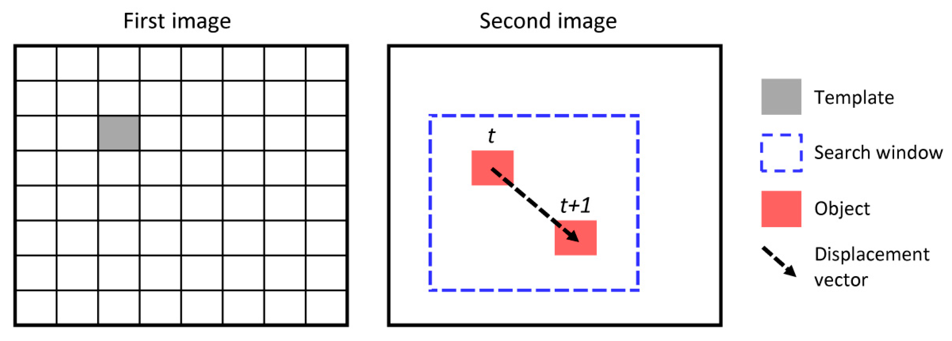
2.1. Maximum Cross-Correlation (MCC) Method Overview

The MCC method aims to detect moving or changing features based on a cross-correlation coefficient. The structural procedure is to cross-correlate a square image subset, referred to as a template, in a first/initial image with all same-sized subsets within the search window of a subsequent image (Figure 1). For all possible subsets in the second/subsequent image, only the one that has the maximum cross-correlation coefficient with the template is considered as the end-point of this transitional motion or change. This procedure produces displacement vectors for every template, but those with low cross-correlation coefficients are considered to be random noise. Thus, a user-defined threshold for the cross-correlation coefficient should be applied to filter the noise [10], and thus, to also retain genuine (valid) change or displacements.
The cross-correlation coefficient is calculated by
ρ ( i , j ) = c o v [ A ( x , y ) , B ( x + i , y + j ) ] v a r [ A ( x , y ) ] v a r [ B ( x + i , y + j ) ]
where A ( x , y ) is the set of pixel values within a template centered at ( x , y ) in an initial image, B ( x + i , y + j ) is the set of pixel values within the corresponding subset in the subsequent image with displacement of ( i , j ) , v a r   [ A ( x , y ) ] and v a r   [ B ( x , y ) ] are variances, and c o v   [ A ( x , y ) , B ( x + i , y + j ) ] is their covariance [10].

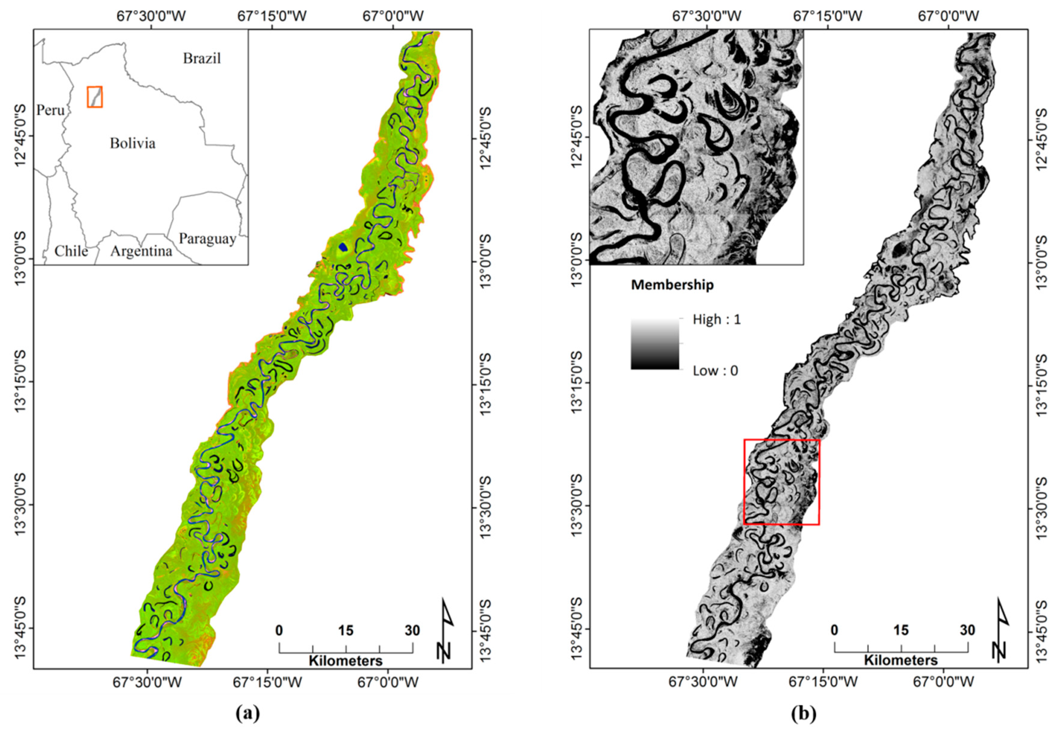
2.2. Data, Pre-Processing, Image Classification, and Classification Accuracy Assessment

The study area is the floodplain of Río Beni, a dynamic tropical meandering river floodplain in northern Bolivia (Figure 2a). Land-cover classes in the study area are spatially heterogeneous, and we considered the following classes: forest, non-forest vegetation, oxbow lake, river, sand, dry soil, and wet soil. In the change-analysis analysis, we utilized three Landsat 5 Thematic Mapper (TM) images (Landsat Level 1T terrain-corrected data were obtained from U.S. Geological Survey (USGS); 30-m pixel size), acquired on 2 August 1987, 27 September 1990, and 5 July 2006, respectively. We analyzed land change within two time periods: (1) from 1987 to 1990; and (2) from 1987 to 2006. The short time period entails relatively modest changes, and thus constitutes a good test of the MCC algorithm as to whether it can detect smaller-magnitude changes, which may be more difficult than detecting larger changes in land cover. Analysis of land change over the long time period provides a more representative characterization of longer-term fluvial landscape dynamics.
We first atmospherically corrected the Landsat 5 TM images to surface reflectance via the Fast Line-of-sight Atmospheric Analysis of Spectral Hypercube (FLAASH®) radiative transfer model [22]. Here, we used a tropical atmospheric model, as well as a rural aerosol model, and for aerosol retrieval, we used a 2-band method [22], involving Landsat 5 TM bands 7 and 3. We then performed supervised fuzzy classification using the FUZCLASS algorithm [23] to derive class membership values for each pixel, where a fuzzy membership image/layer for each land-cover class was generated (e.g., Figure 2b). We distinguished forest and non-forest classes in accordance with the United Nations Food and Agriculture Organization (FAO) definition of forest (i.e., non-agricultural ecosystems with a minimum of 10% crown cover of trees [24]), based on manual/visual image interpretation of reference data (discussed below).
We performed hard classification accuracy assessments, where we jointly used the Landsat TM bands, extracted spectral signatures, computed tasseled-cap images, and high-spatial resolution Google Earth© images as reference data. Prior to the assessment, we hardened fuzzy classification results (i.e., for each pixel, the class with maximum fuzzy membership was used for class assignment). We generated 100 accuracy-assessment sample points per class via stratified random sampling. We computed overall accuracy and the Kappa coefficient [25,26] to assess the accuracy.

2.3. Sensitivity Analysis

We conducted a sensitivity analysis to assess the effectiveness of the MCC method for detecting the direction of land change in terrestrial environments. The MCC method utilizes three important user-defined parameters: template size, search window size (Figure 1), and cross-correlation coefficient threshold. In theory, the size of template is critical, as it controls the range/space over which features can be tracked within a template. An optimal template size should contain enough information for feature tracking, while not being too large so as to minimize noise (i.e., not overgeneralizing or smoothing over too large an area per displacement vector), enabling relatively detailed analyses. The heuristic for the search window size is to set it sufficiently large to accommodate the largest displacement vector expected for a given area/domain, whereas an excessively large search window would lead to unnecessary computation cost. Thus, both the template size and search window size are application domain-specific. In our study, they should be able to capture land change within a large tropical river floodplain. Moreover, the effect of the coefficient threshold on the resultant change/displacement vectors needs attention as well because it directly controls the determination of valid change/displacement vectors. Therefore, we conducted a series of sensitivity analyses to explicitly investigate the influence of MCC parameter values on the MCC results for a terrestrial application, specifically in a dynamic river floodplain environment.
The general test procedure used here was to systematically change/increment an individual parameter value while holding other parameter values constant, and observe the change in the resultant displacement vectors. We evaluated change in displacement vector length, as well as the ratio of the number of valid vectors to the number of possible templates for a given template-size setting. These two variables reflect, respectively, the lengths and distributions of the displacement vectors, and they can be quantitatively recorded and analyzed according to the change in MCC parameters. The length directly indicates the magnitude of displacement related to landscape change; and the ratio describes how many valid vectors are produced according to different parameter settings, which links to how much change information can be collected. Both variables characterize the displacement vectors, including their appearances, and their responses to changes in MCC parameter values illustrate how the three parameters affect the generation of displacement vectors. We also examined the other potentially important factors associated with this application domain, including land-cover class and time period between image acquisitions.
We examined the sensitivity to template size by incrementing the template size by two pixels for each trial over a range from 3 × 3 to 31 × 31 pixels (pixel size = 30 m). We set the search window size to 50 × 50 pixels, which ensured a large search space relative to template size, sufficient to detect actual land-cover transitional change/movement within the time period of interest (i.e., between two multitemporal image acquisitions). We set the MCC threshold to 0.6, which means that a vector is generated only if its maximum cross-correlation coefficient is greater than 0.6. This setting is based on [6], where they conducted an analysis of the relation between a cut-off value (threshold) and the search range, and they demonstrated that a value of 0.6 filtered coincidental pattern matches well (i.e., false displacement vectors) when the search range was less than 5 km. Although their analysis was based on a coastal ocean environment, we utilized this threshold value in the present study as a reference, or baseline, starting point for experiments in this new terrestrial domain. Similarly, to examine the sensitivity to search window size, we used six different search windows ranging from 19 × 19 pixels to 49 × 49 pixels in increments of six pixels. We set the template size to 13 × 13 pixels and MCC threshold to 0.6. In the MCC threshold sensitivity experiment, we used six different thresholds, ranging from 0.5 to 0.9 in increments of 0.1, and set the template size to 13 × 13 pixels, and the search window size to 31 × 31 pixels.
We conducted the sensitivity analysis for each of the seven fuzzy membership maps corresponding to the seven land-cover classes (i.e., forest, non-forest vegetation, oxbow lake, river, sand, dry soil, and wet soil). For each trial, we calculated the average length of valid displacement vectors and the ratio of the number of these vectors to the number of possible templates for a given template size.

3. Results and Discussion

3.1. Classification Accuracy Assessment

Classification accuracy assessments for each of the (hardened) fuzzy image classifications are as follows: overall classification accuracies for images acquired in 1987, 1990, and 2006 are 90.17%, 90.33%, 90.00%, respectively; and the Kappa coefficients for the three images are 0.882, 0.884, 0.880, respectively. The producer’s and user’s accuracies of the land-cover classes are all relatively high; with some of the highest such accuracies being attained for the water and sand classes (Table 1). Note that we merged the river and oxbow-lake classes into one water class prior to accuracy assessment, given their relative spectral similarities.

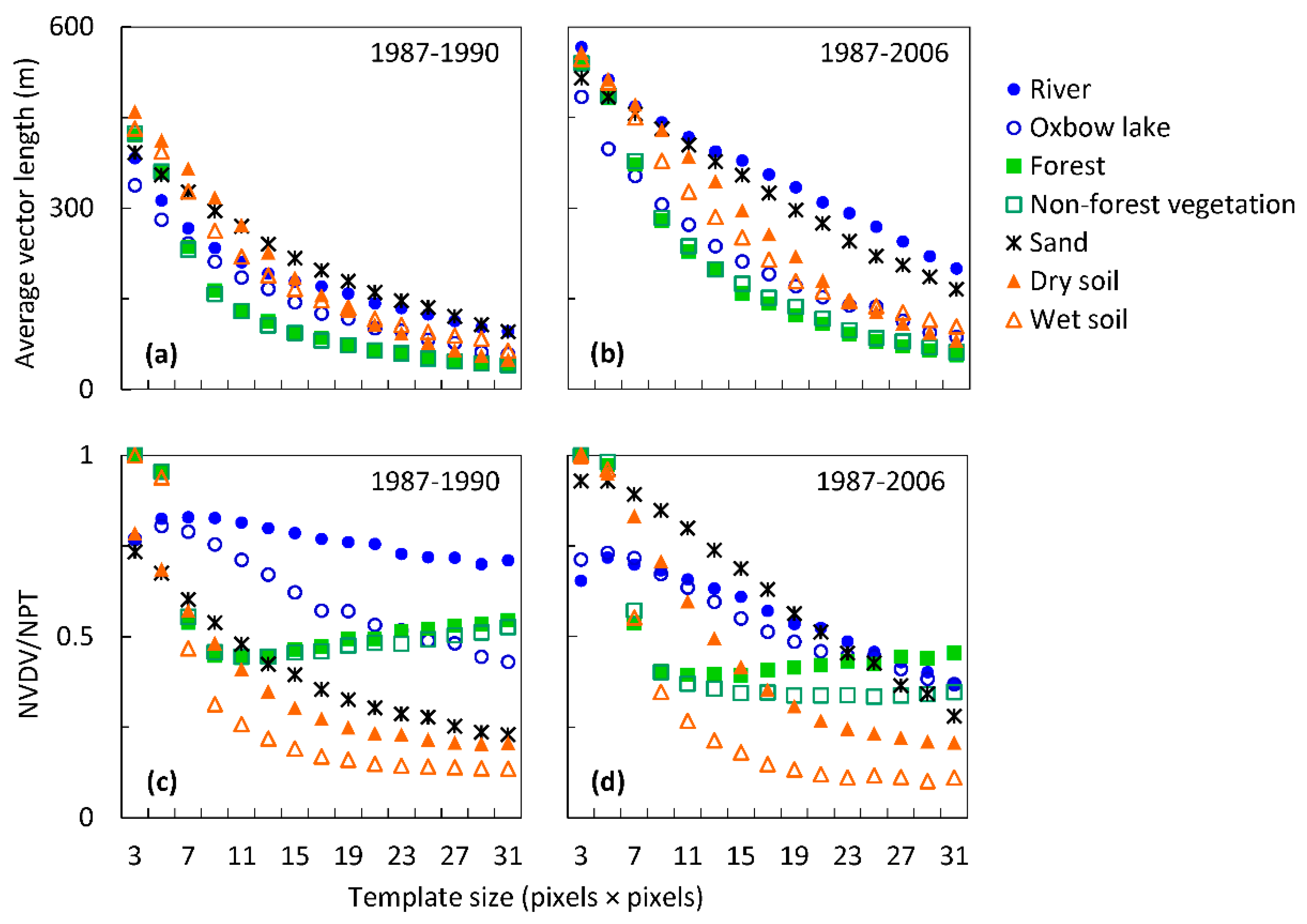
3.2. Sensitivity to Template Size

The average valid displacement vector length over all vectors in the image is high for small template sizes; and as template size increases, the average length decreases (Figure 3). For a small template size, the land-cover patches encompassed within it are also small in extent. Movement of land-cover patches over relatively large distances, or marked changes in areal extent, are possible, yielding a large displacement vector length. However, as template size increases, computed displacement vectors for possibly larger (or even small) land-cover patches within the template would be expected to indicate movement/change over a relatively small distance (or perhaps no movement/change would be detected at all), unless a marked or more dramatic change has occurred during the time period considered. Thus, larger template sizes tend to be less sensitive to changes in the spatial distribution of land-cover patches (Figure 3).
Between 1987 and 1990, some land covers show a decreasing trend, similar to a power function, as the template size increases linearly. For the two vegetation classes, forest and non-forest vegetation, in particular, the downward trends are precipitous over smaller template sizes, yet become relatively stable approximately at template size 11 × 11 pixels (Figure 3). Such trends may be related to landscape spatial scale for these classes. A similar situation exists with the two soil classes, wet and dry soil, though it is not as pronounced as with the vegetation classes. Such phenomena may contribute to the formulation of guidelines for selecting useful template sizes for applications of this nature. Excessively small templates may not capture representative land-cover membership features, whereas very large templates tend to overly smooth features. Furthermore, different land-cover classes may require different template sizes in order to effectively capture the changes. Between 1987 and 2006, the longer time period between the two images analyzed, the overall trends of the various curves look similar to their respective counterparts from the shorter time period (Figure 3). The average lengths of valid displacement vectors are higher than those between 1987 and 1990, which indicates larger-magnitude landscape changes over a longer time period. Additionally, we computed the standard deviation to determine the variability of vector lengths as a function of template size. Results indicate that all seven land-cover classes demonstrate similar patterns, i.e., the variability of vector lengths decreases gradually as the template sizes increase. Also, ranges of vector lengths in all classes show linear decreases as the template sizes increase.
As a given template can only generate one vector, increasing template size must cause a decrease in the vectors produced as the total number of templates decreases. However, this is not necessarily the case for the ratio of the number of valid displacement vectors (NVDV) to the number of possible templates (NPT) for a given template size (Figure 3). The ratio can actually increase as template size increases. The ratio-based patterns for most classes are somewhat similar to those regarding the average valid displacement vector length (Figure 3), which may underscore the importance of selecting an appropriate template size for land-change analysis. That is, both the average valid displacement vector length and ratio of NVDV to NPT change from steep downward trends to more modest, less steep trends after a certain template size is reached; those specific template sizes, or inflection points, may relate to some underlying land process or information.
Across the land-cover classes, there is more variability in the ratio than in the average valid displacement vector length (Figure 3). Between 1987 and 1990, for the two vegetation classes, the ratio decreases rapidly between 3- and 9-pixel template sizes, but then stabilizes at ~0.5 (and then increases slightly) for larger template sizes. The two soil classes exhibit trends somewhat similar to those for vegetation, where there is a steep initial decline in the ratio, and it then stabilizes at ~0.2. The remaining ratio curves indicate only more modest decreases as a function of increasing template size.
In the case of the wet soil class, for example, for template sizes up to ~5 × 5 pixels, >90% of the vectors are valid, meaning that vectors produced by almost all of the templates pass the threshold; thus, there is change detected by nearly all of the templates. As template size increases, there is a dramatic decrease in the number of valid vectors, indicating that there is not a detectable change in most of the templates. Thus, since the sizes of the wet-soil patches are small, smaller template sizes, i.e., no larger than 5 × 5 pixels, are needed to capture change in this class. However, the river class, for example, appears to be less sensitive to the template size. These findings could likely be attributable to the size of the patches of various land-cover classes, as well as possibly the degree of homogeneity of land-cover patches, or features, as indicated by the respective class-specific fuzzy membership layers. The two soil classes only cover small areas within the images, and the fuzzy membership layers for these classes indicate quite small patch sizes, likely translating to higher sensitivities with respect to template size.
There are some notable differences between the results for the short time period and the long: sand and dry soil classes entail higher ratios, whereas the river class has lower ratios relative to the shorter time period. For other land-cover classes, the patterns are similar to those seen between 1987 and 1990 (Figure 3).

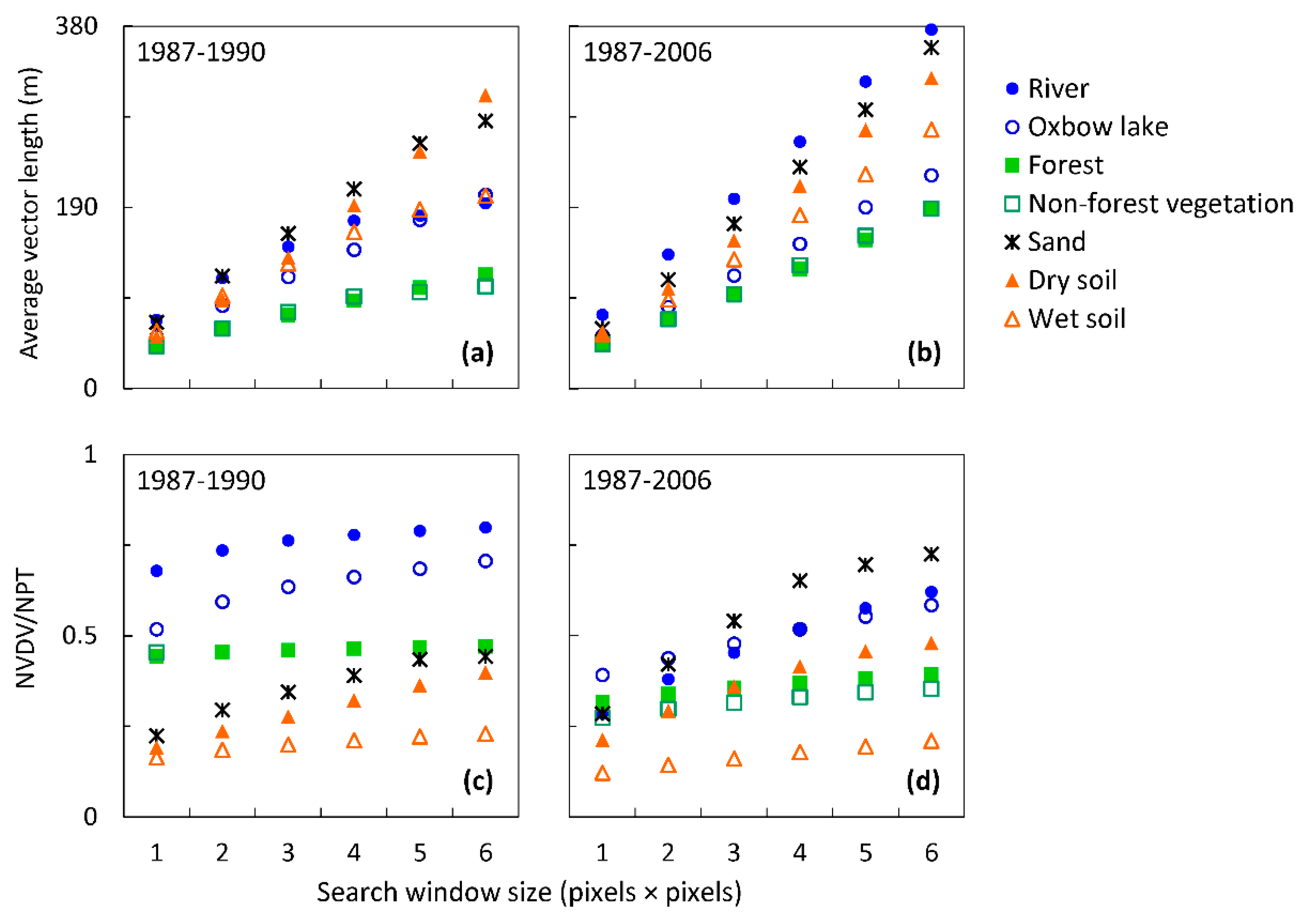
3.3. Sensitivity to Search Window Size

The average valid displacement vector length increases as search window size increases (Figure 4). For the period of 1987–1990, most land-cover classes demonstrate linearly increasing vector lengths with increasing window size, with the exception of vegetation and wet soil classes. Vector lengths for these classes increase but at much slower rate once the search window size reaches at 37 × 37 pixels. Increase in the displacement vector lengths of all land-covers in the shorter time period (1987–1990) is smaller than that in the longer time period (1987–2006) (Figure 4). Also, the change in vector lengths is relatively small (usually about or less than 30 m), considering the ground sampling distance (GSD) or pixel size is 30 m in this image.
Between 1987 and 1990, the ratio of the number of valid displacement vectors (NVDV) to the number of possible templates remains nearly the same for the vegetation classes and wet soil class (Figure 4). For the other land-cover classes, the ratios become stable after about 31 × 31 pixels of search window size. Between 1987 and 2006, the increase in the ratios with increasing search window size is more noticeable compared to that between 1987 and 1990, especially for river and sand classes. However, such increases tend to stabilize beyond a search window size of 37 × 37 pixels (Figure 4).
These results indicate that search window size usually has a minimal effect on the estimation of direction of change if a search window size is sufficiently large to capture transitional movement/change. We recommend conducting experiments on search window size for each given application domain in order to optimize the computation cost and the ability to detect change in features of interest. Based on our experimental results, a search window size set to at least twice the template size appears to be an effective choice for studies performed in similar terrestrial environments.

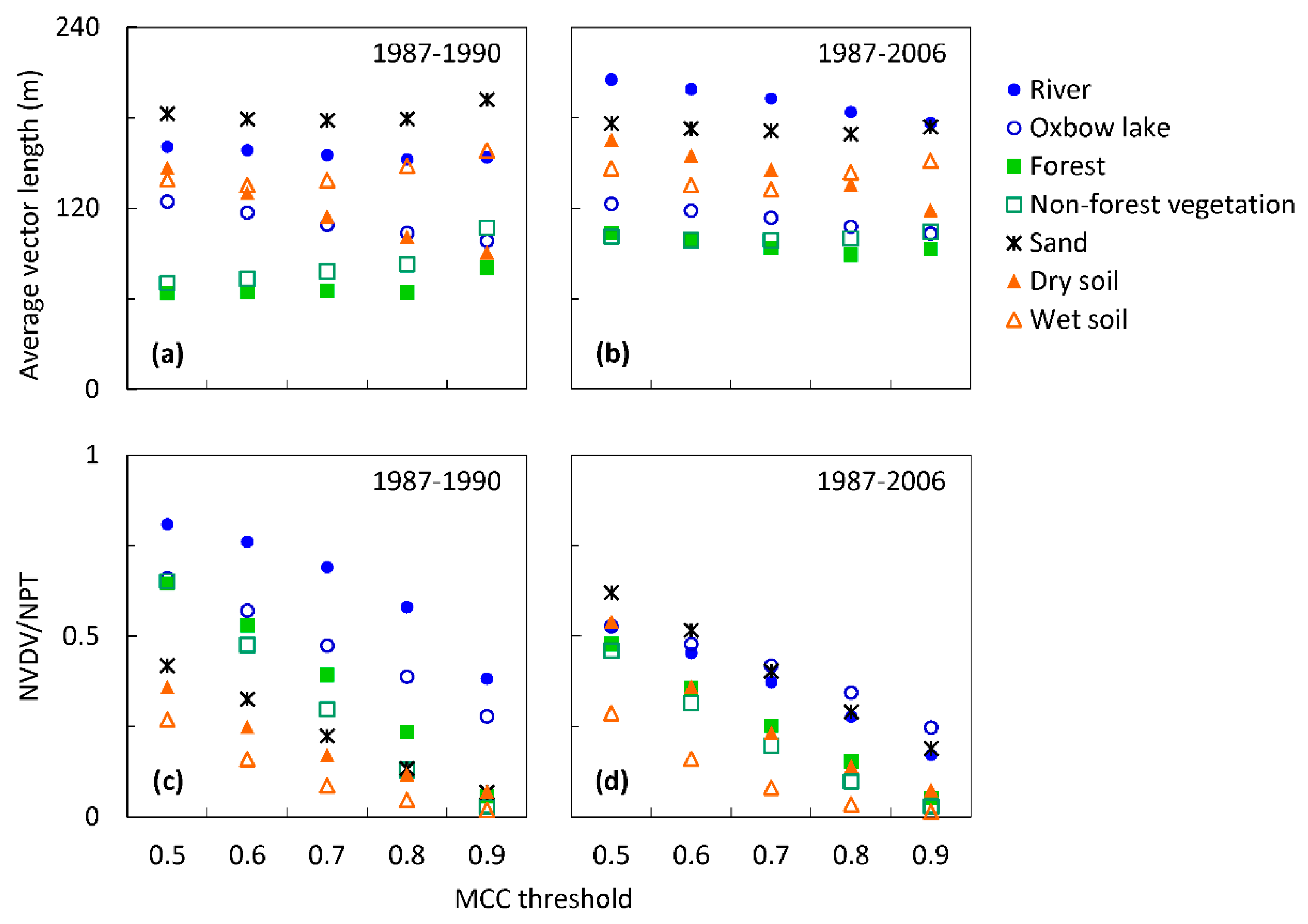
3.4. Sensitivity to MCC Threshold

The sensitivity of the average valid displacement vector lengths to MCC threshold value is low for most land-cover classes, and also for both the shorter (1987–1990) and longer time periods (1987–2006) (Figure 5). There is some variability in the vector lengths for the various land-cover classes for different threshold values; however, considering the 30-m pixel size, the changes exhibited in average valid displacement vector length are not marked as a function of change in the threshold.
The ratio of the NVDV to the NPT for a given template size (13 × 13 pixels, in this case) for all land-cover classes, on the other hand, decreases markedly and linearly as the threshold value increases (Figure 5). Between 1987 and 1990, the initial ratios vary among all land-covers, but all of them drop to below 0.1 (or 10%), except for the two water classes, river and oxbow lake. These water classes have very high vector ratios and still have more than 30% of the templates able to generate change/displacement vectors when the threshold is at 0.9. This means that the change/displacement vectors detected for these two classes usually have very high correlations. However, the two soil classes show relatively low vector percentages. For even the laxest condition, where the threshold is only 0.5, less than 40% of the templates entail valid change/displacement vectors. Between 1987 and 2006, the patterns are similar, but exhibit lower ratios for some of the classes compared with the shorter time period (1987–1990). However, the sand and dry soil classes show higher ratios for both periods. In short, the MCC threshold markedly affects the displacement vectors, as it rules out vectors with MCC below the threshold. Different land-cover membership layers exhibit differing sensitivities to this parameter; thus, this threshold needs to be specified for each land-cover class based on the characteristics of each respective individual membership layer.

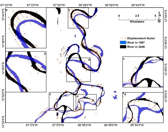
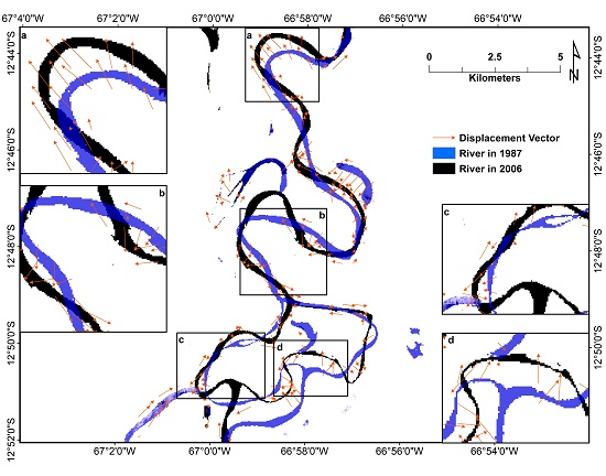
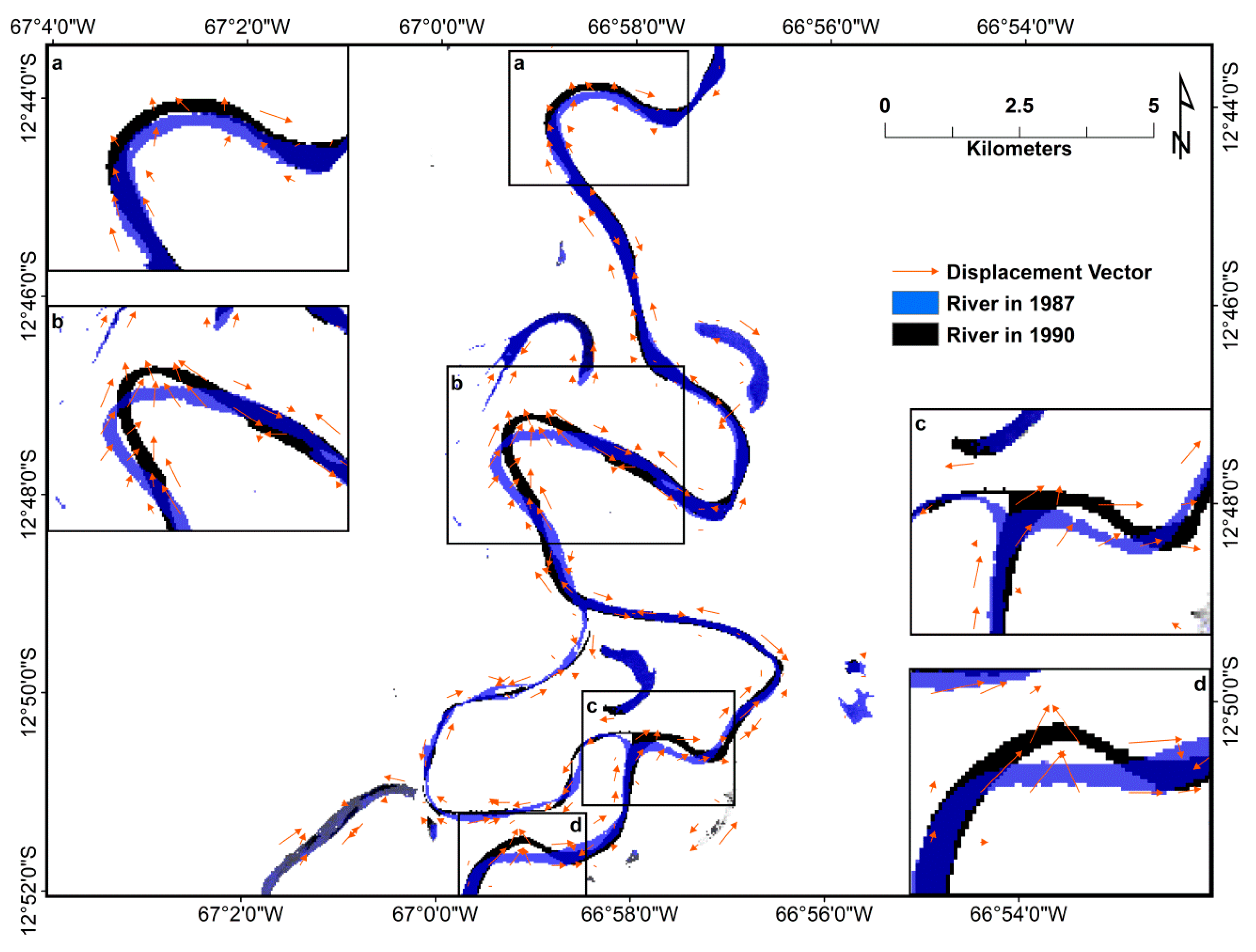
3.5. MCC Land-Change Analysis

Given that the lengths of the displacement vectors are very small compared with the overall size/extent of the Landsat image subsets analyzed here, it is only possible to display in a figure a portion of the study area while still depicting the displacement vectors in a clear manner. Thus, as an example, for a spatial subset of the image/study area where there has been some marked change in the river planform, we present the computed change/displacement vectors resulting from application of the MCC algorithm to the respective river class membership layers from each set of image dates considered (i.e., 1987 and 1990, and 1987 and 2006, respectively). We focus on the river-class change/displacement vectors since the river class is a relatively spatially coherent/homogenous class, represented by well-defined patches; thus, MCC results for this class particularly lend themselves to visual interpretation. However, we also quantitatively summarize the change/displacement vector information via rose diagrams and associated statistics, discussed below. We provide a more detailed view of the change/displacement vectors for a given image pair in four inset sub-windows for selected areas along the river reach (Figure 6 and Figure 7).
In a change-analysis study, an accuracy assessment is typically performed in order to evaluate the performance of a given change-analysis method. A conventional method consists of utilization of per-pixel ground-reference data for the purpose of constructing an error matrix. However, such a method is not suitable to MCC application because the class of change that is detected is not based on individual pixel pairs between images. Some MCC applications that computed ocean current vectors analyzed the accuracies of the MCC method by comparing MCC displacement vectors derived from images to other independent measurements (e.g., Tokmakian et al. [27] compared MCC currents to acoustic Doppler current profiler data and geostrophic velocities computed from dynamic height data). Regarding estimating sea surface velocities from multitemporal satellite images, results indicated that the lowest root-mean-square errors (RMSEs) generated by their MCC implementation when used with real AVHRR satellite images were accrued via averaging three AVHRR fields entailing time separations of 12 h (RMSE = 0.18 m s−1). Experiments involving synthetic images found that, if images that are separated by 6 h are available, such error may be decreased to approximately 0.10–0.15 m∙s−1 [27].) For glacier tracking via the MCC method, comparisons between MCC displacement vectors and actual displacements are not likely, as true displacement data are not usually available for such moving masses [21]. Visualization-based qualitative evaluation is a solution for identifying observable gross errors; however, more quantitative error measurements/metrics for displacement vectors are desired [28]. Debella-Gilo and Kääb [21] devised a method that assumed the Earth surface entities retain their radiometric characteristics after displacement; thus, when comparing the intensities of pixels at the original location and those after displacement in the second image, the difference should be low if the displacement is genuine. However, such a method is not likely to work for general land-cover change, as the algorithm is not necessarily tracking any specific entity; thus, the assumption of radiometric retention or similarity does not hold. So far, there is no standard or established procedure available to quantitatively assess change-analysis accuracy of the MCC algorithm in the terrestrial land-cover domain since the present study constitutes the first such application, to our knowledge. Therefore, in this study, we performed a graphical assessment, involving both the MCC change-analysis results themselves for an example class, as well as a comparison to results from the standard spectral change vector analysis (CVA) algorithm [29], to provide a preliminary indication of change-analysis performance. CVA computes a multi-dimensional change vector in spectral space for each pair of pixels from two images acquired at different times to represent the corresponding change magnitude and direction during this period. Pixels with change magnitude higher than a given threshold are considered as changed pixels, and the “from-to” change class are determined by their change-vector directions. CVA output is a discrete map showing the change status and land-cover class of each pixel. We chose CVA as a baseline, or reference, change-analysis algorithm, as it is a well-established and commonly-used algorithm [30].
In general, we observe that most change/displacement vectors appeared where actual change occurred, and the directions to which the vectors pointed generally matched-up with the prevailing directions of change in the landscape class (river planform, in this case) as assessed via manual image interpretation. Comparing Figure 6 and Figure 7, which were generated based on shorter and longer time-interval image pairs, respectively, we observe that the larger number of vectors and the longer vectors (relative to Figure 6) appear in Figure 7, which is expected, as the river planform experienced more overall change over the longer time period.
Upon close examination of the areas in the inset sub-windows as well as the overall study area, we observe that the lengths of vectors (vector magnitudes) also correspond very well to the exhibited change/displacement within the river class; this appears to provide a new possibility for quantitative characterization of directional and magnitude change of landscape features and related geomorphological processes. However, at least at the level of the information class (i.e., the river class) considered here in this change-analysis, we also observe some apparently incorrect vectors where no actual change occurred or where the directions indicated were incorrect. Most of these instances involve relatively short displacement vectors. These incorrect vectors may potentially be showing change in membership values not associated with actual landscape change (from-to class change), but rather change in intra-class composition (e.g., within-class river water-quality change/variability between two images). Thus, although the MCC change/displacement vectors contain valuable information, for terrestrial landscape change analysis, further consideration regarding filtering is necessary.
For the change period between 1987 and 2006, as an example, the spectral CVA change-analysis overall accuracy is 83.20%, with a Kappa coefficient of 0.664. Figure 8 shows the CVA change pixels associated with the river class, with MCC change/displacement vectors for the same area superimposed on the map. We observe that most of the MCC displacement vectors spatially correspond with the areas that indicate change related to the river according to the CVA result. Also, the directions of the MCC displacement vectors demonstrate good alignment with the change directions of the river channel given by the CVA “from-to” change classes. Thus, the CVA accuracy and the correspondence between CVA and MCC results jointly support the validity of MCC application to a terrestrial landscape—a tropical meandering-river floodplain in this case.
We also examined the distribution of the MCC displacement vectors associated with river channel change for the example river section (Figure 6 and Figure 7) for both time periods. For this purpose, we used the moving average rose diagram (MARD) approach [31], which facilitates emphasizing significant circular trends while reducing background noise. MARD requires two major parameters: the averaging window (or aperture)—i.e., the angular range over which the data are averaged, and a weighting factor that controls the smoothness of plot appearance. We selected an averaging window of 5° and weighting factor of 0.95 based on recommendations in Munro and Blenkinsop [31] and our empirical experimentation. We computed three circular statistics, including vector mean angle, circular variance, and the number of vectors, as well as the mean vector length [31].
For the 1987–1990 period, 194 vectors were observed, with a mean vector length of 230 m, a mean vector angle of 14°, and circular variance of 0.720. On the other hand, for the 1987–2006 period, 189 vectors were computed, with a mean vector length of 435 m, a mean vector angle of 8°, and circular variance of 0.847. The longer time period exhibits a higher circular variance, as well as a markedly higher-magnitude mean vector length, than the shorter time period. We also observed that the vector angles period pointed upwards more frequently than not, indicating that more river channel segments shifted towards the upstream direction during this period. However, in the MARD for the 1987–2006, the displacement vectors have multiple dominant directions (Figure 9). These results correspond with the visualization of the displacement vectors in Figure 6 and Figure 7 and indicate that MARDs and the associated statistics can provide a useful, quantitative summary of the MCC change/displacement vectors.
There have been studies on estimating directional channel change of river planforms using satellite and aerial imagery. For example, Dewan et al. (2017) [32] and Midha and Mathur (2014) [33] studied the channel changes of Ganges and Padma from 1973 to 2011 and of the Sharda River from 1977 to 2001, respectively, using satellite imagery. In both studies, the researchers manually delineated the river-channel boundaries for different dates during the studied period. They then analyzed the movements/shifting directions of river banks on several river transects along the studied channel. Güneralp and Rhoads (2009; 2010) [34,35], for example, also performed a similar type of river planform-change analysis, but employed aerial photography. In contrast, the MCC application proposed in the present study automatically generates directional landscape changes; no manual digitization step is utilized or required, even though manual digitization of river planforms is common practice (e.g., [36]). Yang et al. (2015) [37] determined river-channel migration, or shift, direction, based on sequential satellite images; however, this shifting direction focuses on the migration of the centerline and is only comprised of a “left” or “right” designation. That is, the river shifting direction in [37] is based on the migration area of the centerline (i.e., area enclosed by sequential channel centerlines), where that area is divided into left and right portions relative to the river flow direction, employing the old centerline as the reference. The river shifting direction is determined by which migration is larger—the left or right migration. In contrast, in the present study, MCC displacement vectors are characterized by both a length and angle, as noted above, rather than just returning a nominal directional designation. Thus, the explicit directionality of the MCC method fundamentally differs from the river shifting direction of [37] or any other prior similar study, to our knowledge. Furthermore, and importantly, the landscape changes detected by MCC application are not limited to a single entity type (e.g., a river channel) or certain directions (e.g., along river transects), but may demonstrate directional changes of land-covers that do not have complete or well-defined boundaries. Thus, for any land-cover class or set of land-cover classes of interest, MCC application on terrestrial environments can provide additional and useful information on directional landscape changes compared with traditional change-detection methods.

3.6. Suggestions for Future Research

This implementation of the Maximum Cross-Correlation (MCC) method for change analysis of terrestrial landscapes is unique, and the results in this study indicate distinctive information that can be derived to assist with land-change analysis. However, there are some uncertainties associated with the use of MCC in this domain that should be addressed in future research:
  • An appropriate change-analysis accuracy-assessment procedure needs to be developed for the MCC algorithm in this context. Accuracy assessment is necessary to validate a change-analysis technique. However, given the specialized nature of the combination of the change-analysis method (involving MCC displacement vectors) and the application domain considered, a graphical correspondence assessment was performed in the present research. Although the results of the present research are promising, a more rigorous assessment procedure needs to be developed. Perhaps one possible means of accuracy assessment would be to measure angles and distances/change magnitudes for a given phenomenon, for example, at time t and the same phenomenon at time t + 1. Such measurements could be performed in situ at different times, or perhaps utilizing higher spatial-resolution multitemporal images. Also note that, as discussed in Foody (2004; 2008) [38,39], comparison of accuracies between different methods can be conducted by comparing Kappa coefficients derived from the confusion matrices or other statistical approaches. However, for the MCC application presented here, MCC provides directional change information for quantitative historical land-cover change analysis, which is unlike information produced by other traditional change-detection methods. Thus, a conventional confusion matrix-based assessment method cannot be used to evaluate the accuracy of the directional information contained in the MCC displacement vectors. Based on the MCC results though, from-to class change information could possibly be derived, at least at the template level. Results from other change-detection methods (e.g., CVA) could be generalized via, for example, resampling from the pixel up to the template level, and based on the majority class of the pixels within a given template area. This could potentially allow comparison of MCC class results with those from other change-detection methods. However, again, MCC output is primarily comprised of directional information (i.e., class-by-class spatial displacements across the landscape) in the form of the MCC displacement vectors, which is not comparable to results from traditional change-detection approaches.
  • An improved filtering rule is needed. Besides the MCC threshold, some original MCC applications to ocean currents applied other criteria, e.g., displacement vector length compared with physical movement and velocity of currents in order to filter-out invalid vectors [7]. As noted above, our terrestrial application entailed several invalid vectors that had not been rejected. Thus, a stricter filtering rule based on certain physical/geomorphological/ecological criteria related to the scene is worth investigation in order to eliminate such invalid vectors.
  • Comprehensive interpretation of MCC change/displacement vectors would likely be beneficial. Unlike original ocean-current applications, terrestrial MCC applications contain multiple sets of vectors, where a set of displacement vectors corresponds to a given land-cover class. As different land-cover classes interact with each other during the process of land change, in addition to a separate interpretation for each set of MCC land-cover change/displacement vectors for a given land-cover class, a joint interpretation of multiple or all sets of change/displacement vectors associated with the different respective land-cover classes should be considered. Such a combined analysis may provide a more comprehensive synthesis and assessment of land change. Comprehension of such multifaceted data sets (e.g., regarding how MCC change/displacement vectors represent underlying interactions and processes among multiple land-cover classes) based on visualization will be challenging, and quantitative methods for such joint analyses should thus be a focus of further research. For instance, part of such research may involve converting change/displacement vector information for each fuzzy membership layer into from-to change-analysis information.
  • Finally, note that there are some classes of landscape change for which MCC may not be ideally suited. If a vegetation assemblage, for example, were to completely disappear/be removed from the study area during the time period between two image-acquisition dates, MCC may not capture such a change. Thus, in some such land-change scenarios, MCC may be used in conjunction with other change-analysis algorithms (i.e., pixel- and/or object-based algorithms), with MCC providing a unique and complementary class of change-analysis information.

4. Conclusions

One aspect that has not drawn much attention in land-change analyses to date is the direction of change in land classes of interest. The information on the direction of land-change can be important in situations where, for example, the influence of a hypothesized land-change driver needs to be tested. In this study, we analyze the direction of change in land-cover classes in a floodplain landscape where the land-cover patterns and processes are influenced by a dynamic tropical meandering river. To quantitatively characterize transitional and directional movement of land-covers across the landscape through time, we employ the Maximum Cross-Correlation (MCC) approach, originally developed to track movement of atmospheric, oceanic, and glacial landscape features. Our sensitivity analysis in this first application of MCC to land-change analysis indicates that the results are most sensitive to template size, MCC threshold, and the particular spatial configuration of land-cover classes. Other study areas that one may analyze would almost certainly entail different classes and different spatial configurations of those land-cover classes (relative to the present study). Nevertheless, we posit that the ranges of MCC parameter values tested in this study and the results that were accrued will provide useful guidance for MCC-based directional land-change analyses in the future for similar, and possibly, for other types of environments. Although issues remain associated with the application of MCC to terrestrial environments (e.g., how to effectively assess the accuracy of actual transitional change or movement in a terrestrial environment), this study opens a new avenue for land-change analysis, and presents MCC as a potentially effective method where the direction of change or transition is at least as important as the location of change.

Acknowledgments

The authors thank the anonymous reviewers for their comments and suggestions, which helped to refine and improve the quality of this article.

Author Contributions

M.Y., A.M.F. and İ.G. conceived and designed the experiments; M.Y. performed the experiments; M.Y., A.M.F., İ.G. and B.G. analyzed the data; M.Y., A.M.F., İ.G. and B.G. wrote the paper.

Conflicts of Interest

The authors declare no conflict of interest.

References

  1. Lunetta, R.S.; Johnson, D.M.; Lyon, J.G.; Crotwell, J. Impacts of imagery temporal frequency on land-cover change detection monitoring. Remote Sens. Environ. 2004, 89, 444–454. [Google Scholar] [CrossRef]
  2. Tewkesbury, A.P.; Comber, A.J.; Tate, N.J.; Lamb, A.; Fisher, P.F. A critical synthesis of remotely sensed optical image change detection techniques. Remote Sens. Environ. 2015, 160, 1–14. [Google Scholar] [CrossRef]
  3. Wei, C.; Blaschke, T.; Kazakopoulos, P.; Taubenböck, H.; Tiede, D. Is spatial resolution critical in urbanization velocity analysis? Investigations in the Pearl River Delta. Remote Sens. 2017, 9, 80. [Google Scholar]
  4. Kong, F.; Nakagoshi, N. Spatial-temporal gradient analysis of urban green spaces in Jinan, China. Landsc. Urban Plan. 2006, 78, 147–164. [Google Scholar] [CrossRef]
  5. McGillem, C.D.; Svedlow, M. Image registration error variance as a measure of overlay quality. IEEE Trans. Geosci. Electron. 1976, 14, 44–49. [Google Scholar] [CrossRef]
  6. Bowen, M.M.; Emery, W.J.; Wilkin, J.L.; Tildesley, P.C.; Barton, I.J.; Knewtson, R. Extracting multiyear surface currents from sequential thermal imagery using the maximum cross-correlation technique. J. Atmos. Ocean. Technol. 2002, 19, 1665–1676. [Google Scholar] [CrossRef]
  7. Crocker, R.I.; Matthews, D.K.; Emery, W.J.; Baldwin, D.G. Computing coastal ocean surface currents from infrared and ocean color satellite imagery. IEEE Trans. Geosci. Remote Sens. 2007, 45, 435–447. [Google Scholar] [CrossRef]
  8. Crocker, R.I.; Matthews, D.K.; Emery, W.J.; Qazi, W.A.; Baldwin, D. Near-Realtime U.S. Coastal Ocean Surface Currents Derived From Sequential Thermal Satellite Imagery. Available online: http://ccar.colorado.edu/colors/mcc.html (accessed on 27 September 2016).
  9. Emery, W.J.; Thomas, A.C.; Collins, M.J.; Crawford, W.R.; Mackas, D.L. An objective method for computing advective surface velocities from sequential infrared satellite images. J. Geophys. Res. 1986, 91, 12865–12878. [Google Scholar] [CrossRef]
  10. Gao, J.; Lythe, M.B. The maximum cross-correlation approach to detecting translational motions from sequential remote-sensing images. Comput. Geosci. 1996, 22, 525–534. [Google Scholar] [CrossRef]
  11. Leese, J.A.; Novak, C.S.; Clark, B.B. An automated technique for obtaining cloud motion from geosynchronous satellite data using cross correlation. J. Appl. Meteorol. 1971, 10, 118–132. [Google Scholar] [CrossRef]
  12. Ninnis, R.M.; Emery, W.J.; Collins, M.J. Automated extraction of pack ice motion from advanced very high resolution radiometer imagery. J. Geophys. Res. 1986, 91, 10725. [Google Scholar] [CrossRef]
  13. Civco, D.L.; Hurd, J.D.; Wilson, E.H.; Song, M.; Zhang, Z. A comparison of land use and land cover change detection methods. In Proceedings of the ASPRS-ACSM Annual Conference, Washington, DC, USA, 22–26 April 2002. [Google Scholar]
  14. Kim, J.G. Assessment of recent industrialization in wetlands near Ulsan, Korea. J. Paleolimnol. 2005, 33, 433–444. [Google Scholar] [CrossRef]
  15. Im, J.; Jensen, J.; Tullis, J. Object-based change detection using correlation image analysis and image segmentation. Int. J. Remote Sens. 2008, 29, 399–423. [Google Scholar] [CrossRef]
  16. Koeln, G.; Bissonnette, J. Cross-correlation analysis: Mapping landcover change with a historic landcover database and a recent, single-date multispectral image. In Proceedings of the 2000 ASPRS Annual Convention, Washington, DC, USA, 22–26 May 2000. [Google Scholar]
  17. Hurd, J.D.; Wilson, E.H.; Lammey, S.G.; Civco, D.L. Characterization of forest fragmentation and urban sprawl using time sequential Landsat imagery. In Proceedings of the ASPRS Annual Convention, St. Louis, MO, USA, 23–27 April 2001. [Google Scholar]
  18. Moughal, T.A.; Yu, F.; Mazher, A.; Liu, S.; Razzaq, A. Enhanced detection of burned area using cross- and autocorrelation. J. Appl. Remote Sens. 2015, 9, 096018. [Google Scholar] [CrossRef]
  19. Tarantino, C.; Adamo, M.; Lucas, R.; Blonda, P. Detection of changes in semi-natural grasslands by cross correlation analysis with WorldView-2 images and new Landsat 8 data. Remote Sens. Environ. 2016, 175, 65–72. [Google Scholar] [CrossRef] [PubMed]
  20. Im, J.; Jensen, J.R. A change detection model based on neighborhood correlation image analysis and decision tree classification. Remote Sens. Environ. 2005, 99, 326–340. [Google Scholar] [CrossRef]
  21. Debella-Gilo, M.; Kääb, A. Locally adaptive template sizes for matching repeat images of Earth surface mass movements. ISPRS J. Photogramm. Remote Sens. 2012, 69, 10–28. [Google Scholar] [CrossRef]
  22. Perkins, T.; Adler-Golden, S.; Matthew, M.; Berk, A.; Anderson, G.; Gardner, J.; Felde, G. Retrieval of atmospheric properties from hyper- and multi-spectral imagery with the FLAASH atmospheric correction algorithm. Proc. SPIE 2005, 5979. [Google Scholar] [CrossRef]
  23. Eastman, J.R. IDRISI Taiga Guide to GIS and Image Processing; Clark Labs Clark University: Worcester, MA, USA, 2009. [Google Scholar]
  24. Food Agriculture Organization (FAO). Forest Resources Assessment 1990. Tropical Countries; FAO: Rome, Italy, 1993. [Google Scholar]
  25. Congalton, R.G. A review of assessing the accuracy of classifications of remotely sensed data. Remote Sens. Environ. 1991, 37, 35–46. [Google Scholar] [CrossRef]
  26. Congalton, R.G.; Green, K. Assessing the Accuracy of Remotely Sensed Data: Principles and Practices; CRC Press/Taylor & Francis: Boca Raton, FL, USA, 2009. [Google Scholar]
  27. Tokmakian, R.; Strub, P.T.; McClean-Padman, J. Evaluation of the maximum cross-correlation method of estimating sea surface velocities from sequential satellite images. J. Atmos. Ocean. Technol. 1990, 7, 852–865. [Google Scholar] [CrossRef]
  28. Evans, A.N. Glacier surface motion computation from digital image séquences. IEEE Trans. Geosci. Remote Sens. 2000, 38, 1064–1072. [Google Scholar] [CrossRef] [Green Version]
  29. Malila, W.A. Change vector analysis: An approach for detecting forest changes with Landsat. In Proceedings of the LARS Symposia, Purdue University, Lafayette, IN, USA, 3–6 June 1980. [Google Scholar]
  30. Baker, C.; Lawrence, R.; Montagne, C.; Patten, D. Change detection of wetland ecosystems using Landsat imagery and change vector analysis. Wetlands 2007, 27, 610–619. [Google Scholar] [CrossRef]
  31. Munro, M.A.; Blenkinsop, T.G. MARD—A moving average rose diagram application for the geosciences. Comput. Geosci. 2012, 49, 112–120. [Google Scholar] [CrossRef]
  32. Dewan, A.; Corner, R.; Saleem, A.; Rahman, M.M.; Haider, M.R.; Rahman, M.M.; Sarker, M.H. Assessing channel changes of the Ganges-Padma River system in Bangladesh using Landsat and hydrological data. Geomorphology 2017, 276, 257–279. [Google Scholar] [CrossRef]
  33. Midha, N.; Mathur, P.K. Channel characteristics and planform dynamics in the Indian Terai, Sharda River. Environ. Manag. 2014, 53, 120–134. [Google Scholar] [CrossRef] [PubMed]
  34. Güneralp, İ.; Rhoads, B.L. Empirical analysis of planform curvature–migration relation of meandering rivers. Water Resour. Res. 2009, 45, W09424. [Google Scholar] [CrossRef]
  35. Güneralp, İ.; Rhoads, B.L. Spatial autoregressive structure of meander evolution revisited. Geomorphology 2010, 120, 91–106. [Google Scholar] [CrossRef]
  36. Gupta, N.; Atkinson, P.M.; Carling, P.A. Decadal length changes in the fluvial planform of the River Ganga: Bringing a mega-river to life with Landsat archives. Remote Sens. Lett. 2013, 4, 1–9. [Google Scholar] [CrossRef]
  37. Yang, C.; Cai, X.; Wang, X.; Yan, R.; Zhang, T.; Zhang, Q.; Lu, X. Remotely sensed trajectory analysis of channel migration in Lower Jingjiang Reach during the period of 1983–2013. Remote Sens. 2015, 7, 16241–16256. [Google Scholar] [CrossRef]
  38. Foody, G.M. Thematic map comparison: Evaluating the statistical significance of differences in classification accuracy. Photogramm. Eng. Remote Sens. 2004, 70, 627–633. [Google Scholar] [CrossRef]
  39. Foody, G.M. Harshness in image classification accuracy assessment. Int. J. Remote Sens. 2008, 29, 3137–3158. [Google Scholar] [CrossRef]
Figure 1. Depiction of the Maximum Cross-Correlation (MCC) method, including a template, search window, and displacement vector. Example feature (in red) within a given template extent at time t is shown, as is the direction and magnitude of shift in the feature position at time t + 1, relative to that at time t (after [6]).
Remotesensing 09 00850 g001
Figure 2. (a) Landsat 5 Thematic Mapper (TM) image of the study area, acquired on 2 August 1987, with bands 4,5,1 as R,G,B (pixel size = 30 m); (b) fuzzy membership image for the forest class, with example enlarged spatial subset given in the upper left to facilitate illustration of floodplain complexity, and location of spatial subset designated by red box. The study area extends between approximately 12°31′34′′ and 13°49′19′′ South latitude, and between 66°54′04′′ and 67°32′05′′ West longitude, an area comprising ~2060 km2.
Remotesensing 09 00850 g002
Figure 3. Sensitivity of MCC method to template size. Average valid displacement vector length for the periods of (a) 1987–1990 and (b) 1987–2006 and the ratio of the number of valid displacement vectors (NVDV) to the number of possible templates (NPT) for the periods of (c) 1987–1990 and (d) 1987–2006 as a function of template size. Search window size = 50 × 50 pixels, MCC threshold = 0.6.
Remotesensing 09 00850 g003
Figure 4. Sensitivity of MCC method to search window size. Average valid displacement vector length for the periods of (a) 1987–1990 and (b) 1987–2006, and the ratio of the number of valid displacement vectors (NVDV) to the number of possible templates (NPT) for the periods of (c) 1987–1990 and (d) 1987–2006 as a function of search window size. Template size = 13 × 13 pixels, MCC threshold = 0.6.
Remotesensing 09 00850 g004
Figure 5. Sensitivity of MCC method to MCC threshold. Average valid displacement vector length for the periods of (a) 1987–1990 and (b) 1987–2006, and the ratio of the number of valid displacement vectors (NVDV) to the number of possible templates (NPT) for the periods of (c) 1987–1990 and (d) 1987–2006 as a function of MCC threshold. Template size = 13 × 13 pixels, search window size = 31 × 31 pixels.
Remotesensing 09 00850 g005
Figure 6. River class-membership images for 1987 and 1990, and MCC vectors (in red) derived from this pair of images. The 1987 river layer and the 1990 river layer (after change) are shown in blue and black, respectively (blue is 30% transparent and overlaid on black layer). Four inset zoom-in windows along the figure margins correspond to their respective specific areas along the river reach, identified by their corresponding labels (ad).
Remotesensing 09 00850 g006
Figure 7. River class-membership images for 1987 and 2006, and MCC vectors (in red) derived from this pair of images. The 1987 river layer and the 2006 river layer (after change) are shown in blue and black, respectively (blue is 30% transparent and overlaid on black layer). Four inset zoom-in windows along the figure margins correspond to their respective specific areas along the river reach, identified by their corresponding labels (ad).
Remotesensing 09 00850 g007
Figure 8. CVA result associated with the river class for the time period 1987 to 2006, with MCC vectors (in red) derived from this pair of images. As determined by CVA, pixels that changed from the river class over this time period are colored green, whereas pixels that changed to the river class are in blue. Four inset zoom-in windows along the figure margins correspond to their respective specific areas along the river reach, identified by their corresponding labels (ad).
Remotesensing 09 00850 g008
Figure 9. Moving average rose diagrams (MARDs) summarizing the MCC change/displacement vectors for the river class within the example river reach given in Figure 7 and Figure 8, for the periods of (a) 1987–1990; and (b) 1987–2006. Values on the radar plot axes indicate average weighted frequencies of azimuths.
Remotesensing 09 00850 g009
Table 1. Producer’s and user’s classification accuracies for the (hardened) fuzzy classified Landsat images acquired in 1987, 1990, and 2006, respectively.
Accuracy (%)Year
198719902006
Overall90.1790.3390.00
By land cover classProducer’sUser’sProducer’sUser’sProducer’sUser’s
Forest90.9190.0085.3293.0086.1193.00
Non-forest vegetation84.3186.0087.7686.0083.0083.00
River and oxbow lake86.21100.0094.34100.0095.24100.00
Sand100.0090.0095.8893.00100.0092.00
Dry soil88.4692.0091.5887.0090.7078.00
Wet soil93.2683.0087.3783.0078.9086.00
Kappa coefficient0.8820.8840.880

