Article

Atmospheric Correction of Multi-Spectral Littoral Images Using a PHOTONS/AERONET-Based Regional Aerosol Model

1
Univ. Bordeaux, UMR 5805, EPOC, Environnements et Paléoenvironnements Océaniques et Continentaux, 33615 Pessac, France
2
CNES, CNRS, IRD, Univ. Toulouse, UMR 5126, CESBIO, Centre d’Etudes Spatiales de la BIOsphère, 31401 Toulouse, France
3
Univ. Bourgogne, UMR 6282, Biogéosciences, 21000 Dijon, France
4
Univ. Littoral Cote d’Opale, Univ. Lille, CNRS, UMR 8187, LOG, Laboratoire d’Océanologie et de Géosciences, 62930 Wimereux, France
*
Author to whom correspondence should be addressed.
Remote Sens. 2017, 9(8), 814; https://doi.org/10.3390/rs9080814
Submission received: 29 June 2017 / Revised: 1 August 2017 / Accepted: 4 August 2017 / Published: 8 August 2017
(This article belongs to the Special Issue Atmospheric Correction of Remote Sensing Data)

Abstract

:
Spatial resolution is the main instrumental requirement for the multi-spectral optical space missions that address the scientific issues of marine coastal systems. This spatial resolution should be at least decametric. Aquatic color data processing associated with these environments requires specific atmospheric corrections (AC) suitable for the spectral characteristics of high spatial resolution sensors (HRS) as well as the high range of atmospheric and marine optical properties. The objective of the present study is to develop and demonstrate the potential of a ground-based AC approach adaptable to any HRS for regional monitoring and security of littoral systems. The in Situ-based Atmospheric CORrection (SACOR) algorithm is based on simulations provided by a Successive Order of Scattering code (SOS), which is constrained by a simple regional aerosol particle model (RAM). This RAM is defined from the mixture of a standard tropospheric and maritime aerosol type. The RAM is derived from the following two processes. The first process involved the analysis of a 6-year data set composed of aerosol optical and microphysical properties acquired through the ground-based PHOTONS/AERONET network located at Arcachon (France). The second process was related to aerosol climatology using the NOAA hybrid single-particle Lagrangian integrated trajectory (HYSPLIT) model. Results show that aerosols have a bimodal particle size distribution regardless of the season and are mainly represented by a mixed coastal continental type. Furthermore, the results indicate that aerosols originate from both the Atlantic Ocean (53.6%) and Continental Europe (46.4%). Based on these results, absorbing biomass burning, urban-industrial and desert dust particles have not been considered although they represent on average 19% of the occurrences. This represents the main current limitation of the RAM. An assessment of the performances of SACOR is then performed by inter-comparing the water-leaving reflectance ( ρ w ) retrievals with three different AC methods (ACOLITE, MACCS and 6SV using three different standard aerosol types) using match-ups (N = 8) composed of Landsat-8/Operational Land Imager (OLI) scenes and field radiometric measurements. Results indicate consistency with the SWIR-based ACOLITE method, which shows the best performance, except in the green channel where SACOR matches well with the in-situ data (relative error of 7%). In conclusion, the study demonstrates the high potential of the SACOR approach for the retrieval of ρ w . In the future, the method could be improved by using an adaptive aerosol model, which may select the most relevant local aerosol model following the origin of the atmospheric air mass, and could be applied to the latest HRS (Sentinel-2/MSI, SPOT6-7, Pleiades 1A-1B).

Graphical Abstract

1. Introduction

Marine coastal social–ecological systems are dramatically exposed to the adverse effects of global environmental changes and anthropogenic drivers [1,2]. To cope with disaster risks, develop appropriate responses (such as climate adaptation and mitigation policies) and improve risk governance, decision-makers need timely and useful information for the assessment of coastal vulnerability [3,4,5]. Satellite remote sensing is a crucial component of Earth observation programs to support this objective. Aquatic color radiometry (ACR) particularly offers one of the most spatially and temporally comprehensive tools for the monitoring of the littoral environment and assessment of security [6,7].
Marine coastal systems are characterized by spatially heterogeneous biological, physical, geochemical and geomorphological features and controlling processes [8]. Due to a low spatial resolution, ocean color sensors, such as MODIS (Moderate Resolution Imaging Spectroradiometer) or OLCI (Ocean and Land Color Instrument), show limited capabilities in progressing from the measurements of key environmental parameters to quantitatively interpreting the associated processes [9]. To address scientific issues associated with these environments, high spatial resolution satellite remote sensors (HRS) are required. Although HRS space programs are generally primarily designed for the monitoring of continental surfaces, recent decametric spatial resolution missions (Landsat-8/Operational Land Imager (OLI) or Sentinel-2/Multi-Spectral Instrument (MSI)) demonstrate a high potential for littoral applications due to improved instrument capacities [10,11]. On the other hand, sub-decametric missions show limited capacities particularly due to lower spectral characteristics (for instance, no near-infrared (NIR) or short-wave infrared (SWIR) bands to support accurate atmospheric corrections). The major importance of sub-decametric HRS data for the monitoring of marine coastal systems [8,12] requires the development of a specific atmospheric correction in processing.
The use of ACR data to estimate key aquatic environmental parameters (e.g., suspended particulate matter, chlorophyll-a concentration, water depth and benthic habitat) involves accurate atmospheric corrections (AC) for deriving the water-leaving reflectance ( ρ w ) from the top-of-atmosphere signal ( ρ T O A ) recorded by sensors. This signal is mainly dominated by the gaseous and aerosol contributions of the atmosphere. While the contribution of air molecules is well considered [13,14], the aerosol contribution still generates high uncertainties in the correction of atmospheric effects due to the difficulty to accurately estimating the concentration and type of atmospheric particles. Typical AC methods for the processing of ACR data over open ocean areas use the signal measured at NIR wavelengths in order to determine the aerosol model. This assumes a zero value of ρ w in this spectral region due to a high light absorption by pure water compared to the light backscattering by suspended particles [15] (noted GW94 thereafter). In coastal waters, the contribution of the particle backscattering at NIR wavelengths is no longer negligible [16,17,18]. To solve this problem, different AC approaches have been proposed based on: (i) the use of SWIR [17,19] or ultraviolet [20,21] spectral bands; (ii) the spatial homogeneity of the NIR band ratio [13,16,22]; (iii) the spectral shape matching method [23,24,25,26]; or (iv) direct neural networks inversion [27,28] and adding constraints to the GW94 scheme for taking into account a non-zero water-leaving reflectance [29,30,31,32,33,34]. However, the requirement for spectral bands at the NIR and SWIR wavelengths for HRS space missions severely limits these approaches.
Furthermore, marine coastal environments are characterized by a high dynamic range of concentration and type of aerosols. In particular, the Atlantic coast exhibits marked temporal and spatial variability in the microphysical and optical properties of atmospheric particles due to various sources of continental and maritime aerosols [35]. Maritime aerosols are generally non-absorbing and are mainly composed of sea salt particles produced from the breakup of water bubbles. Continental aerosols may be roughly divided into urban-industrial, Saharan dust and biomass burning types [36]. Urban-industrial aerosols are characterized by a significant spatial and temporal variability of its two main contributors, namely the non-absorbing sulfate and absorbing carbon particles. As for the biomass burning type, absorbing urban-industrial aerosols are composed in particular of black carbon, which have a strong absorption in the near-infrared wavelengths. Mineral dust particles, which are a major component of Saharan dust, show high absorption in the blue wavelengths, while a lower absorption is observed in the other spectral regions. Typical AC methods are based on a limited number of aerosol models, which fail to represent all local aerosol conditions and thus, directly impact the accuracy of retrievals [37,38,39]. The limited number of aerosol models is particularly true for the AC methods used to process the surface reflectance of standard decametric space missions, which have been provided by the U.S. Geological Survey (USGS) for OLI [40] and the Theia Land Data Center for MSI [14].
To overcome these limitations, one relevant alternative solution is to directly derive the contribution of aerosols using radiative transfer simulations obtained from the use of an accurate regional aerosol model [39]. We believe that this regional approach is fully justified in the context of operational monitoring of environmental security with regards to an increased number of global approaches. In this paper, we describe the development of the in Situ-based Atmospheric CORrection (SACOR) approach, which is adaptable to individual sites. The regional aerosol model (RAM) is developed following the methodology of Ahmad et al. [38] and using the combined analysis of the two following processes. The first involves a 6-year data set composed of aerosol optical and microphysical properties acquired through the ground-based PHOTONS/AERONET network located at Arcachon, while the second is related to aerosol climatology using the NOAA hybrid single-particle Lagrangian integrated trajectory (HYSPLIT) model. While SACOR can be applied to any HRS data, results are presented for the OLI data in order to evaluate and inter-compare the performances of the algorithm with respect to the SWIR- and NIR-based ACOLITE [19] and MACCS (Multi-Sensor Atmospheric Correction and Cloud Screening processor) [14] algorithms. To highlight the impact of the aerosol model, additional comparisons are performed on ρ w retrievals using the Second Simulation of a Satellite Signal in the Solar Spectrum (6SV) radiative transfer code with standard atmospheric particle models.

2. Materials and Methods

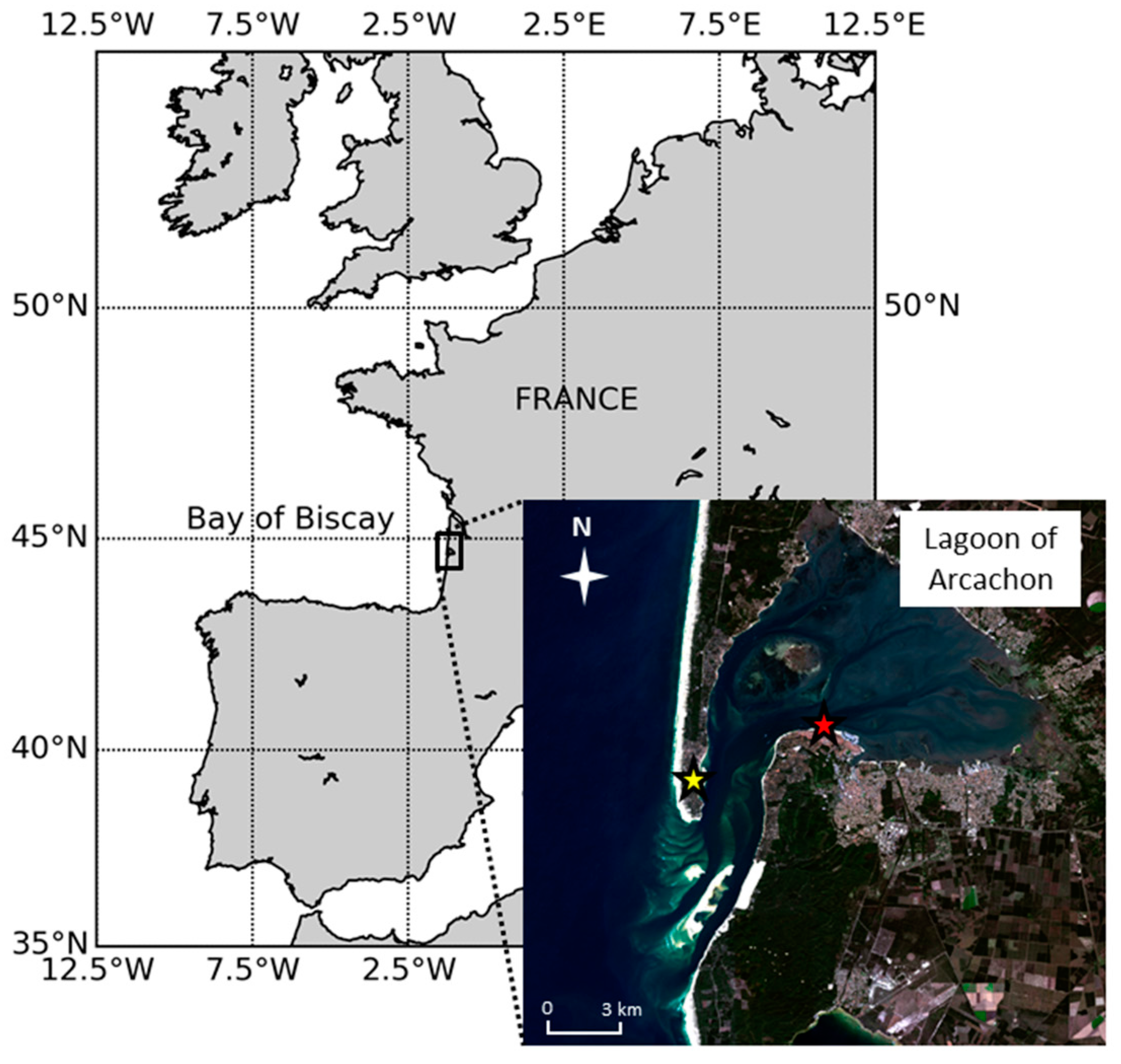
2.1. Site Description

Arcachon Bay is a macrotidal shallow semi-enclosed lagoon of approximately 180 km2 located on the French Atlantic coast (44°40′N, 1°10′W; Figure 1). It is connected to the Atlantic Ocean by a channel that is 2–3 km wide and about 12 km long. Waters are optically complex and present a high turbidity gradient associated with the salinity gradient. The spatial heterogeneity of the suspended particulate and dissolved matter in terms of composition and concentration is mainly determined by oceanic inputs and river discharges in the external and inner part of the lagoon, respectively, which is coupled with moderate water renewal rates [41,42,43]. Biogeochemical parameters of the water column are also characterized by a high temporal variability. Over the period of 2005–2015, the mean annual values of the concentration of suspended particulate matter (SPM), chlorophyll-a (Chl) and particulate organic carbon to nitrogen ratio (C/N ratio, proxy of the origin of SPM) are 4.06 ± 4.56 mg/L, 1.53 ± 0.79 μg/L, and 5.75 ± 1.74 mol/mol, respectively, at the Comprian station (COMP) located in the inner part of the lagoon (statistics extracted from the data set of the French Coastal Monitoring Network SOMLIT).
The climate in the Arcachon area is mild. The summer is hot and dry, while the winter is rainy and cold. The mean maximum temperature in summer ranges from 21.0 to 24.0 °C, while this temperature ranges from 10.9 to 12.2 °C in winter. Similarly, the mean minimum temperature in summer ranges from 12.1 to 15.1 °C, while this temperature ranges from 2.5 to 3.2 °C in winter. The maximum monthly average value of relative humidity is observed in January (82 ± 3%), while the minimum value is seen in July (71 ± 2%) (statistics extracted from the data set of Météo-France, Lège-Cap Ferret station). On the Earth surface, northwesterly winds dominate on average from spring to late summer, while southwesterly winds dominate from autumn to early spring [44]. However, winds present a significant variability associated with four well-defined atmospheric circulation patterns [45], which directly impact the aerosol concentration and types. The main origin of primary aerosols emitted in the Arcachon area derives mainly from oceanic (fresh sea-spray droplets), biotic stress-induced (humid area and pine forest), biomass burning and vehicular emissions [46].

2.2. AERONET Data

Optical and microphysical properties of the aerosols over the area are derived from sun and sky radiance measurements acquired from a ground-based CIMEL CE-318 photometer. The CIMEL located at Arcachon has been operational since September 2008 under collaboration between the LOA (University of Lille) and the EPOC (University of Bordeaux) laboratories. Calibrations of the instrument are carried out by the French National Observatory Network for Aerosol (PHOTONS), which is a part of the Aerosol Robotic Network (AERONET). The standardized AERONET procedures of the instrumentation, methodology, data processing and data quality control are fully described in previous studies [35,47,48,49]. For this study, we used mean daily quality-assured level 2.0 data from January 2009–May 2015 in order to define the aerosol model. Specifically, as mentioned in Section 2, the seasonal behavior of both direct sun (aerosol optical depth at 500 nm (AOD) and Ångström coefficient computed between 440 and 870 nm ( α 440 870 )) and inversion products (aerosol particle size distribution (PSD) and AOD fine mode fraction (FMF)) is analyzed to infer the dominant aerosol types.
The accuracy of AERONET retrievals was investigated in numerous studies [47,48,49,50]. Good performances were reported for the AOD and PSD. Values of PSD are retrieved in 22 equidistance bins in the ln(r) space, where r varies from 0.05 to 15 μm. The errors for PSD do not exceed 10% in the maxima of the intermediate particle size range (0.1 ≤ r ≤ 7 μm), while the estimated uncertainty for AOD is approximately ±0.01 for λ ≥ 400 nm. The single scattering albedo (SSA) and complex index of refraction (n) retrievals can be accurately retrieved only for high aerosol loading (AOD(440) ≥ 0.5). However, for the AERONET Arcachon site, 97.5% of the data (on a total of 991 averaged daily observations) did not report SSA and n values. Consequently, the SSA observations can not be used in this study for determining the nature of aerosol. Finally, the estimation of the AOD fine mode fraction, FMF, was reported as a robust process, which is based on the separation of the AOD into fine and coarse contributions [50].

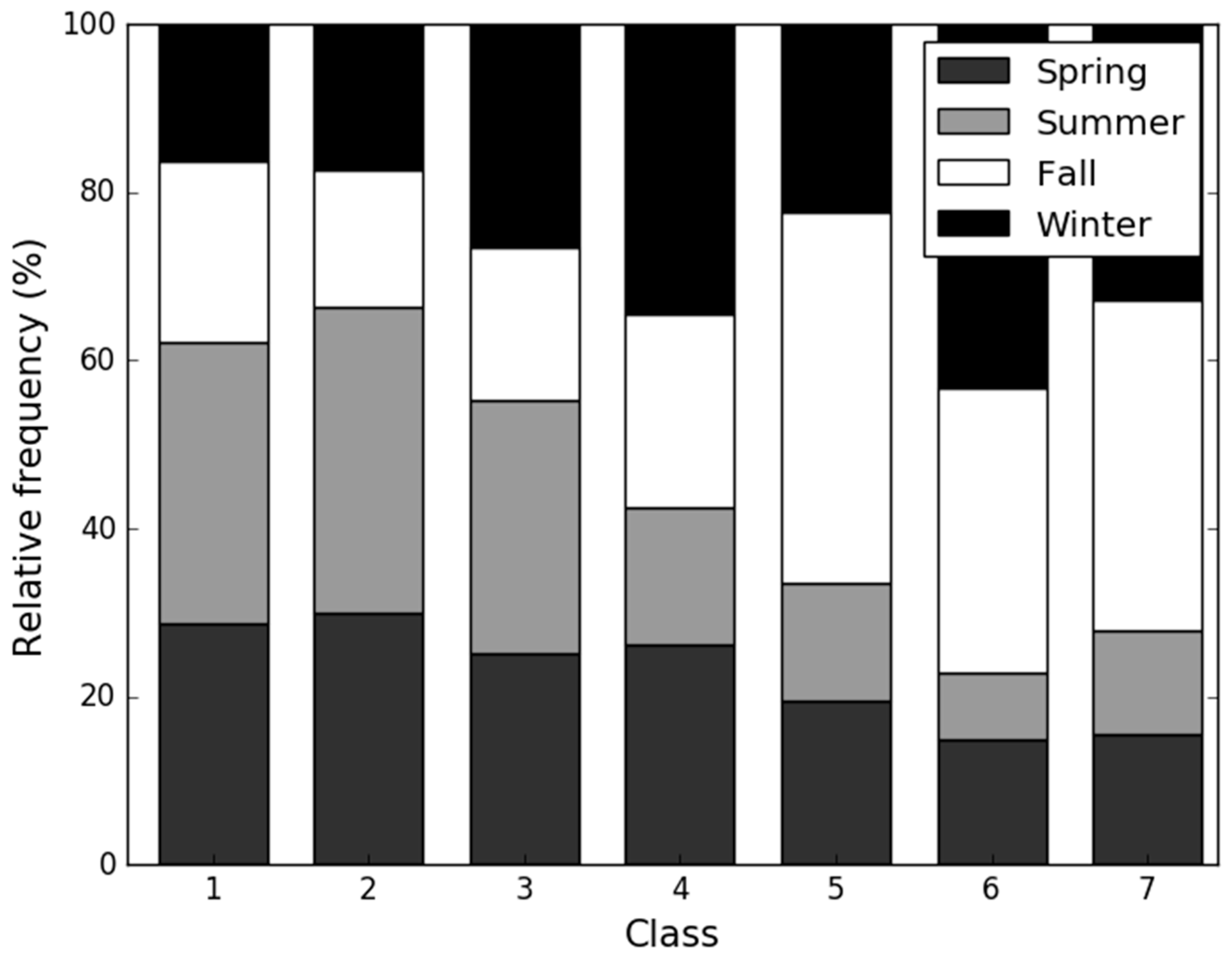
2.3. Classification of Air Masses back Trajectories

In addition to the CIMEL data analysis, air mass back trajectories ending at Arcachon at 12:00 UTC have been computed with the NOAA Hybrid Single-Particle Lagrangian Integrated Trajectory (HYSPLIT) model [51,52,53] in order to investigate the origin of the aerosols. From 1 January 2009 to 31 December 2015, a three-day back trajectory was calculated for each day. A calculation of the back trajectories limited to 72 h back is based on a compromise between the need to reduce the uncertainties caused by the meteorological conditions [54] and the consideration of regional and long-range transport. Back trajectories were performed for two different altitude levels (1000 and 3000 m), which served as representations of the air masses in the boundary layer and in the free troposphere. In all, more than 5000 trajectories were produced. The NCEP Global Data Assimilation System (GDAS) dataset was downloaded and used as meteorological inputs. To identify the dominant patterns of back trajectories, a cluster analysis is performed using the options included into the HYSPLIT software. The cluster analysis is based on the total spatial variance (TSV) method [55,56,57]. The variation of TSV was used to determine the optimal number of clusters or classes.

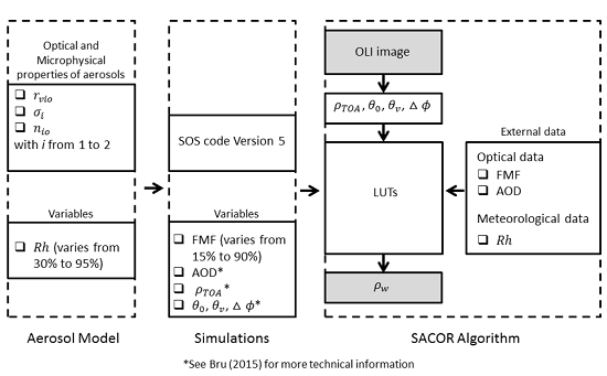
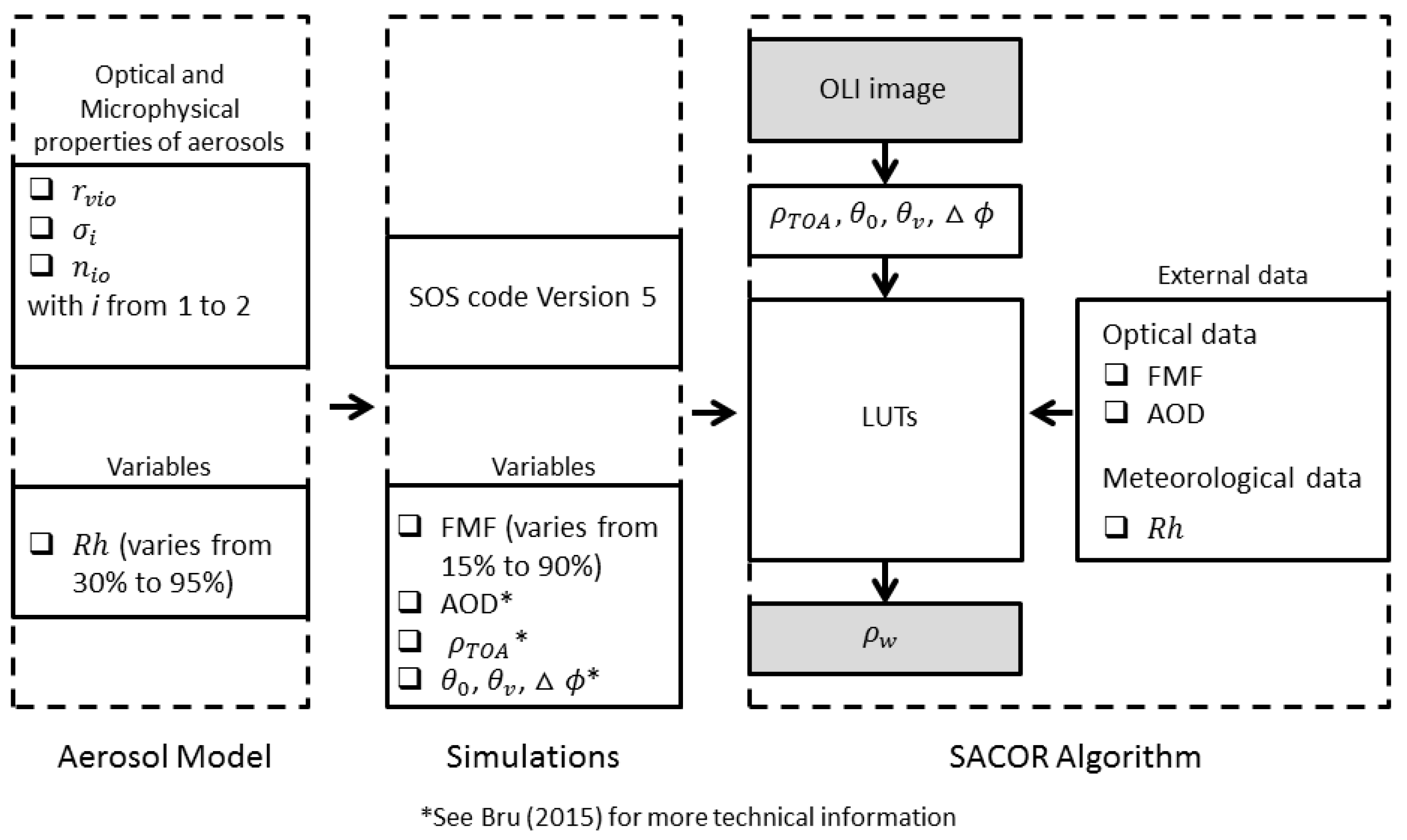
2.4. The In-Situ Based Atmospheric CORrection Algorithm (SACOR)

2.4.1. Algorithm Description

After pre-processing of sun glint, whitecaps and gaseous absorptions [58], the top-of-atmosphere reflectance ( ρ T O A ( λ ) ) measured by multi-spectral optical sensors can be approximately expressed as follows [15]:
ρ T O A ( λ ) = ρ r ( λ ) + ρ a ( λ ) + ρ r a ( λ ) + t ( λ ) . ρ w ( λ ) ,
where λ is the wavelength; ρ r ( λ ) is the reflectance due to scattering by the air molecules; ρ a ( λ ) is the reflectance due to the scattering by aerosols; ρ r a ( λ ) is the reflectance due to the multiple scattering from the interaction between molecules and aerosols; ρ w ( λ ) is the water-leaving reflectance; and t ( λ ) is the two-way diffuse atmospheric transmittance. Note that the impact of the spherical albedo is neglected in this study due to its small effect on the contributions from the water body [59,60]. For brevity, we suppress the reference to the spectral dependency in the following text.
Most of the algorithms used to remove the atmospheric signal due to aerosols from ρ T O A are based on posteriori knowledge of the aerosol types derived from the analysis of the ρ T O A spectral shape at NIR and SWIR wavelengths. Following the method developed by Ahmad et al. [38], we propose an alternative approach for regional applications. The SACOR approach presented in this paper allows for estimation of the aerosol contribution to ρ T O A from a priori knowledge of the aerosol nature (i.e., their microphysical and optical properties) and using the in-situ data from ground-based instruments. Thus, the SACOR methodology is based on the definition of an appropriate aerosol model used to generate a set of lookup tables (LUTs) from an exact radiative transfer code with suitable input parameters as described in the following section.
Aerosol models are fully described by three microphysical and optical parameters of atmospheric particles, which are the volume geometric mean radius ( r v i ), the geometric standard deviation ( σ i ) and the complex index of refraction ( n i ). The subscript i refers to the ith mode of the PSD. The most appropriate model for the PSD is a bimodal lognormal distribution where the first and second modes are generally associated with fine and coarse particles, respectively [47]. Note that r v i and σ i allow for calculation of PSD using the following expression:
d V ( r ) d l n ( r ) = i = 1 2 V i 2 π σ i e x p [ ( ln ( r ) ln ( r v i ) 2 σ i ) 2 ] ,
where r is the volume geometric mean radius of the particle and V i is the volume of the particles associated with the ith mode.
As reported by Ahmad et al. [38], r v i and n i are closely dependent on the relative humidity, which is denoted by Rh [61,62]. Hanel [61] provides the models for computing these parameters as a function of Rh:
r v i ( R h ) = r v i 0 [ 1 + ρ m w ( R h ) m i 0 ] 3 ,
n i ( R h ) = n w + ( n i 0 n w ) [ r v i 0 r v i ( R h ) ] 3 ,
where r v i 0 and n i 0 are the radius and complex index of refraction at Rh = 0, respectively; m i 0 is the mass of dry particle; m w and n w are the mass and the complex index of refraction of condensed water, respectively; and ρ is the ratio of wet-to-dry mass density of aerosols. Based on Equations (2)–(4), the aerosol model explicitly depends only on Rh when the values of r v i 0 , n i 0 , σ i and V i are known. In our approach, the values of r v i 0 and n i 0 are determined using the literature [62] once the aerosol model is defined. These values have been used for more than a decade in the standard atmospheric correction of the SeaWiFS and MODIS images. The determination of the most representative aerosol model described in Section 3.3 is based on a long-time series analysis of in-situ AOD, α 440 870 and PSD observations supported by a climatology study aiming to identify the aerosol origins at a synoptic scale. The σ i value is determined as the average value of all AERONET monthly means computed at Arcachon, as shown by Ahmad et al. [38].
Following this, LUTs associated with the aerosol model are generated from the Successive Order of Scattering code V5 (SOS) [63,64]. It is important to note that the gaseous absorption is not considered by the SOS code. For this process, we used the SMAC code (Small Method for Atmospheric Correction; [65]) and the coefficient values associated with OLI, which were provided by the CESBIO (Centre d’Etudes Spatiales de la BIOsphere). To reproduce the high range of variability in the atmospheric optical properties, viewing and solar geometry conditions, simulations are performed using different values of V i computed from FMF (i.e., the ratio of the fine mode to the total AOD), AOD, ρ T O A , Rh, zenith sun angle ( θ 0 ), zenith viewing angle ( θ v ) and azimuth difference ( Δ ϕ ) (technical information are provided in a previous study [66]). These variables are used as input parameters in the SACOR algorithm to select the correct LUTs. As ρ T O A , θ 0 , θ v and Δ ϕ can be directly extracted from OLI images, the SACOR algorithm requires only three external data types, namely Rh, AOD and FMF, which could be provided by ground-based observations. Figure 2 gives a schematic representation of the SACOR algorithm.

2.4.2. Assessment of SACOR performances

The SACOR approach can be applied to any HRS space mission data as the set of LUTs can be generated for any sensor spectral characteristics. However, in this study, OLI was selected to evaluate the performances of our approach for different reasons. First, OLI shows a high potential for coastal applications due to the improved instrument capacities [10,13,67]. Following this, AC algorithms with good performance have been developed for aquatic color applications [20]. OLI is a push-broom imager launched in February 2013 to continue Landsat’s mission of Earth system monitoring. OLI images consist of 8 spectral bands with a spatial resolution of 30 m, with 4 bands in the visible wavelength as well as 3 bands at the NIR and SWIR wavelengths. The sensor provides radiometrically robust observations for coastal environments [10] with a signal-to-noise-ratio (SNR) that is higher than 200 in the visible, NIR and SWIR bands. The Level 1T (Terrain corrected) OLI products were downloaded from the Landsat-8 USGS portal [68].
Evaluation of the SACOR performances is based on the comparison of ρ w retrievals from our method with: (i) in-situ measurements and (ii) atmospherically corrected reflectance provided by standard AC algorithms. The methodology follows a two-step process. In the first step, the atmospherically corrected OLI data are validated using the in-situ ρ w recorded within a short time interval of ±30 min with regards to the satellite overpass time in order to limit the impact of the tide on the match-up quality. Due to challenging meteorological conditions, only eight match-ups associated with four OLI scenes are used in this study despite there being 16 field campaigns conducted between 7 March 2014 and 7 December 2015 (Figure 3). Table 1 provides information about OLI images and associated aerosol conditions, which unfortunately show a low diversity. For each match-up, the satellite-derived ρ w is computed as the average value over a 3-by-3 pixel box centered on the in-situ station [18,39] and the in-situ ρ w spectrum is adjusted to match the L8/OLI channels using their relative spectral response (RSR) functions [10]. In the second step, a qualitative assessment of the robustness of SACOR is performed over a wide range of bio-optical conditions. Evaluation is based on the comparison of the SACOR and SWIR-based ACOLITE atmospherically corrected products along a cross-shore transection [69].
In-situ hyperspectral radiometric measurements using TriOS-RAMSES sensors were regularly recorded at the SOMLIT stations (COMP, TES and B13; see Figure 3) during field cruises aboard the French oceanographic vessel Planula IV (CNRS/INSU), which have been planned in order to correspond with the Landsat-8 overpass time. The location of SOMLIT stations allows for sampling of a spatial gradient of seawater optical properties. The station COMP located in the inner part of the Arcachon lagoon has optical properties that are mainly influenced by fresh waters coming from tributaries, while the optical properties at the station B13 located in the west part of the inlet are influenced by coastal waters [42]. Field measurements include the in-water upwelling radiance ( L u ( z ) , where z is the depth), above-water upwelling radiance ( L s e a 0 + ), sky radiance ( L s k y 0 + ) and downwelling irradiance ( E d 0 + ). The remote-sensing reflectance ( R r s ) is then computed using the above- and in-water protocols described by Ruddick et al. [70] and Lubac and Loisel [71], respectively. The field above-water R r s measurements are selected for match-up when the mean relative difference between the above- and in-water R r s spectrums (computed over the 400–950 nm wavelength interval) is lower than 5%. This criterion ensures high-quality measurements. Following this, ρ w was then determined as:
ρ w = π R r s ,
The standard AC methods used for the inter-comparison of ρ w retrievals with SACOR are the ACOLITE algorithm (https://odnature.naturalsciences.be/remsem/software-and-data/acolite [20]); MACCS (Multi-Sensor Atmospheric Correction and Cloud Screening processor [14]); and the 6SV (Second Simulation of a Satellite Signal in the Solar Spectrum Vector code [72]) code compiled for three different types of standard atmospheric particles (continental, maritime and tropospheric). ACOLITE is developed at the RBINS (Royal Belgian Institute of Natural Sciences). This image-based model does not require external data. AC is based on the determination of the aerosol type (ε) using the ratio of Rayleigh corrected reflectance in the Red, NIR or SWIR bands because it can be assumed that ρ w is null with respect to the level of turbidity [13,20]. Spectral ε is then used to interpolate the aerosol contribution in the visible bands. In this paper, the per-tile fixed epsilon option is selected for the NIR and SWIR algorithms (thereafter noted ACO-NIR and ACO-SWIR, respectively), as it has been shown to provide better results than the per-pixel variable epsilon [69].
The L2A OLI products provided by Theia [73] were processed with the MACCS method, which has been fully described by Hagolle et al. [74]. AOD is derived from the image, using a combination of three methods: the black pixel method, the dark dense vegetation method (DDV) and the multi-temporal (MT) method. The black pixel method is used to find the maximum value of AOD in the image. The DDV method is used to estimate the amount of aerosol by coupling the surface reflectance above vegetation in the Red and Blue bands. Finally, the MT method is based on the assumptions that aerosols vary quickly in time but not with location, while surface reflectance varies with location but slowly in time. Any changes between two images can be related to aerosols which allows for the aerosol contribution to be estimated. Surface reflectance is estimated using LUTs built with the Successive Orders of Scattering (SOS) code.
The 6SV1.1 is an operational source code allowing the simulation of the surface reflectance under a variety of atmospheric, spectral and geometrical conditions. The code is based on the SOS model and is also capable of accounting for radiation polarization [75]. The microphysical characteristics of the aerosol models account for dry particles.
For the SACOR and 6SV methods, OLI images were processed from L1T to L2 using CIMEL (AOD, FMF and water vapor) and meteorological (Rh) data. For the MACCS method, downloaded images were already corrected. In contrast to the other algorithms, MACCS method involves an adjacency effect correction.

3. Results and Discussion

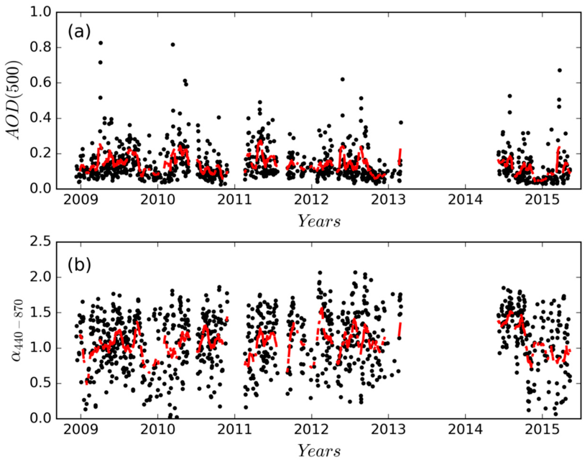
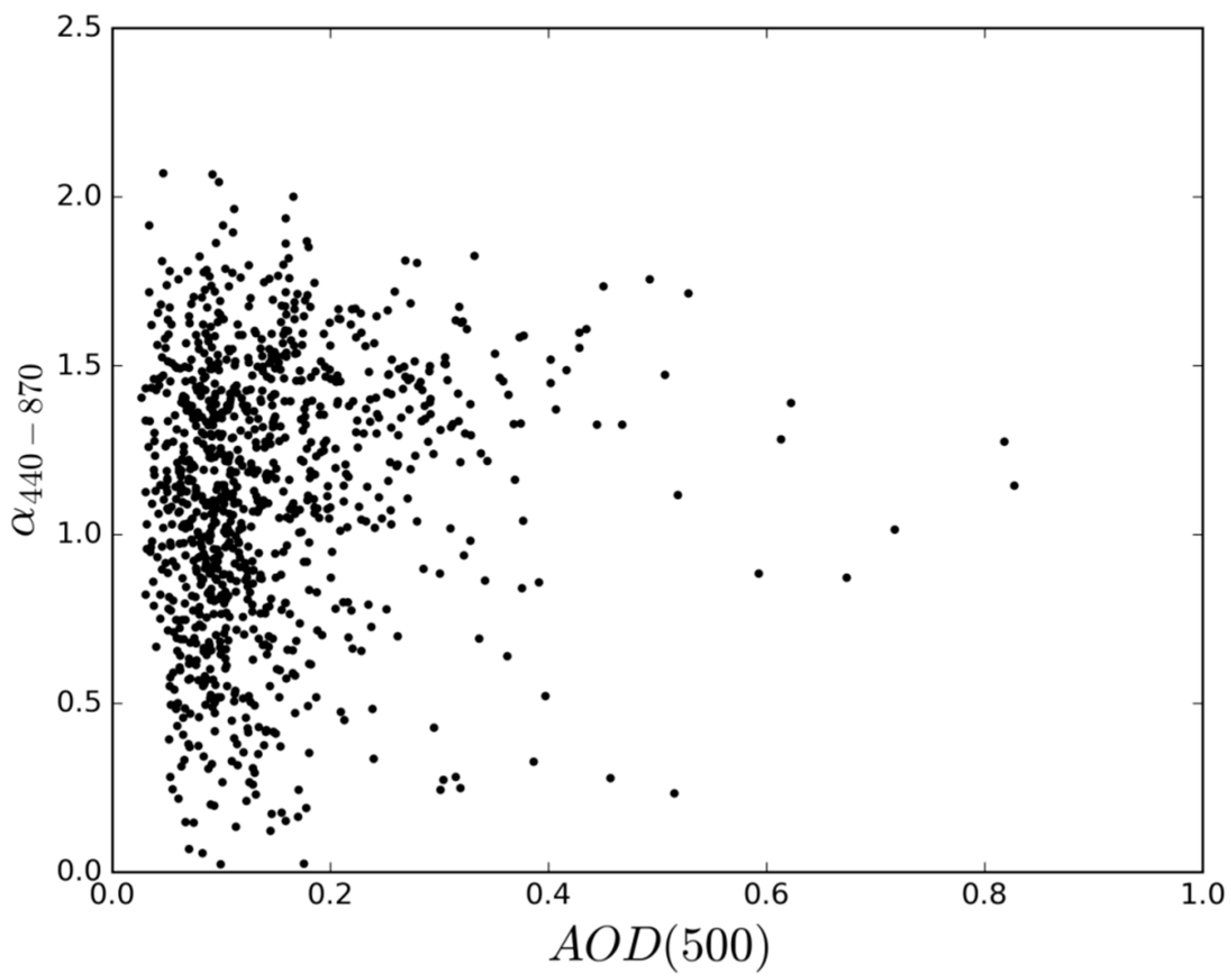
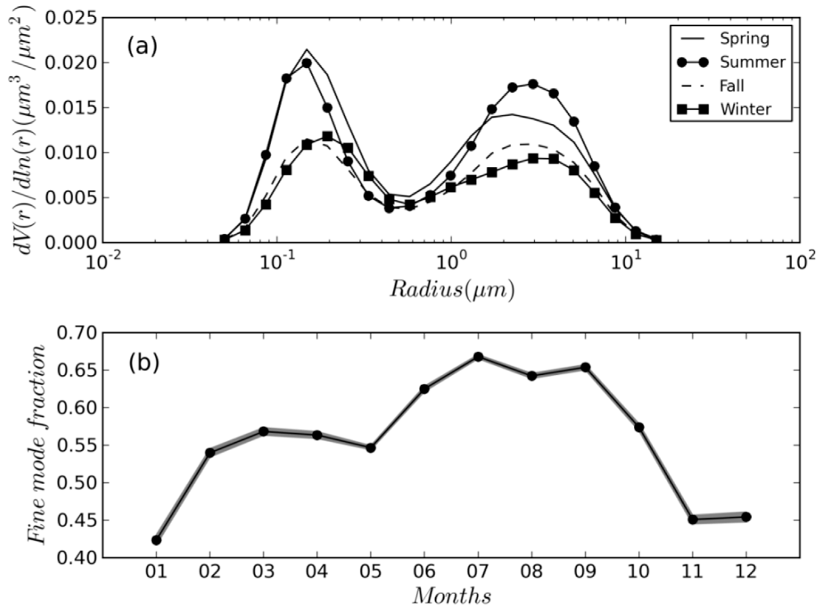
3.1. Variability of Aerosol Optical and Microphysical Properties

Figure 4 shows daily mean values of the aerosol optical depth at 500 nm (AOD) and the Ångström coefficient ( α 440 870 ) from December 2008 to May 2015. A total of 991 observations are reported in Figure 4. As cloud cover is typically greater in the fall (October, November and December) and winter (January, February and March), there are more cloud-free observations in spring (April, May and June) and summer (July, August and September) (Table 2). It is worth mentioning that some gaps can be observed in the measurement record due to electrical/mechanical failures and sensor malfunctions (June–July 2010; December 2010–February 2011; August–September 2011) as well as the change in the local CIMEL technical support team (March 2013–June 2014).
AOD (Figure 4a) and α 440 870 (Figure 4b) have a significant seasonal variability. The maximum values of AOD are observed in spring and summer with mean values of 0.18 ± 0.11 and 0.14 ± 0.08 (Table 2), respectively. The minimum values are observed in fall and winter with mean values of 0.11 ± 0.06 and 0.10 ± 0.10. This seasonal behavior could be attributed to a higher wildland fire activity and long-range transport from the Eastern Europe in spring and summer [76]. There are also higher rainfalls in fall and winter, which cause washout and wet depositions of aerosol [77,78]. Similarly, the maximum seasonal values of α 440 870 are observed in spring (with a mean value of 1.11 ± 0.36) and summer (1.20 ± 0.36), while minimum values are observed in fall (1.08 ± 0.41) and winter (1.07 ± 0.47). This seasonal behavior indicates a higher aerosol fine fraction in spring and summer, which is probably due to a high-volume contribution of biomass burning aerosols. This is higher compared to fall and winter where winter storms lead to an increase in the coarse fraction due to enhanced production of sea-salt particle.
The behavior of α 440 870 as a function of AOD is shown in Figure 5. The α 440 870 –AOD scatter plot allows the discrimination of different aerosol types, as reported in a large number of studies (see references in [79,80]). The determination of the aerosol types is based on threshold values, which are highly dependent on the relevant site [81]. In this study, threshold values are defined from the local aerosol climatology provided by Smirnov et al. [35] and Dubovik et al. [36] as well as the classification created by Toledano et al. [82] and Kaskaoutis et al. [83]. These threshold values are used to distinguish three pure aerosol types (clean maritime (CM); biomass burning and urban-industrial (BU); and desert dust (DU) models), and two mixed types (mixed maritime (MM) and mixed continental (MC) models). The selected threshold values of α 440 870 and AOD for each aerosol type are reported in Table 2. Following this classification, aerosols at the Arcachon lagoon mainly fall into the MC type (50%), which can be associated with coastal continental aerosols that are optically characterized by the influence of the local sources of maritime and polluted aerosols. A total of 31% of the observations is associated with maritime types (17% and 14% for CM and MM, respectively), while 15% and 4% of the observations are associated with the BU and DU types. A high seasonal variation in the proportion of the different types of aerosols can be observed, except for the MM aerosol type with its proportion ranging from 17% in spring to 11% in summer. The influence of MC types is dominant during all seasons, although there is a more balanced contribution in spring (39%) and winter (45%) compared to summer (61%) and fall (54%). CM aerosols show a higher contribution in fall and winter with a frequency of 23% and 26%, respectively, while these aerosols have a lower contribution in spring and summer (14% and 9%). The BU and DU types contribute more to the total number of aerosols in spring (22% and 8%), while the minimum contributions are found in fall and winter.
Figure 6 shows the seasonal microphysical properties of aerosols at the AERONET Arcachon lagoon station calculated during the period from December 2008 to May 2015. As expected for a high proportion of mixed aerosols, the particle volume size distribution (Figure 6a) is bimodal regardless of the season. The fine (with a peak value located between 0.15–0.19 μm) and coarse (2.24–2.94 μm) modes reveal a high variability. The peak magnitudes of the fine and coarse modes range from 0.013 (in fall) to 0.021 μm3/μm2 (in spring) and 0.008 (in winter) to 0.020 μm3/μm2 (in summer), respectively. Figure 6b shows the mean monthly fine mode fraction, which can be considered as a proxy of the contribution (%) of fine particles to the total AOD. The minimum values are observed in the months of winter and fall with a mean of 47% and 55%, respectively. The maximum values are found in the months of summer (65%) and spring (56%). The dominant variations in these distributions can be directly associated with changes in optical conditions and aerosol types. These results are consistent with the highest proportion of CM aerosols and the lowest α 440 870 values previously observed in winter as well as the highest proportions of BU and DU aerosols and the highest α 440 870 values observed in spring and summer (Table 2). Finally, a comparison between the mean value of FMF at the AERONET Arcachon lagoon station and two other AERONET coastal sites (Chesapeake Bay and Dunkerque in Northwest France) is performed (results not presented in this paper). It is worth noting that the Arcachon site presents a lower proportion of fine particles (58%) compared to the two other coastal sites (approximately 64%), which indicates a higher influence of particles originating from the Atlantic area (results presented in [66]).

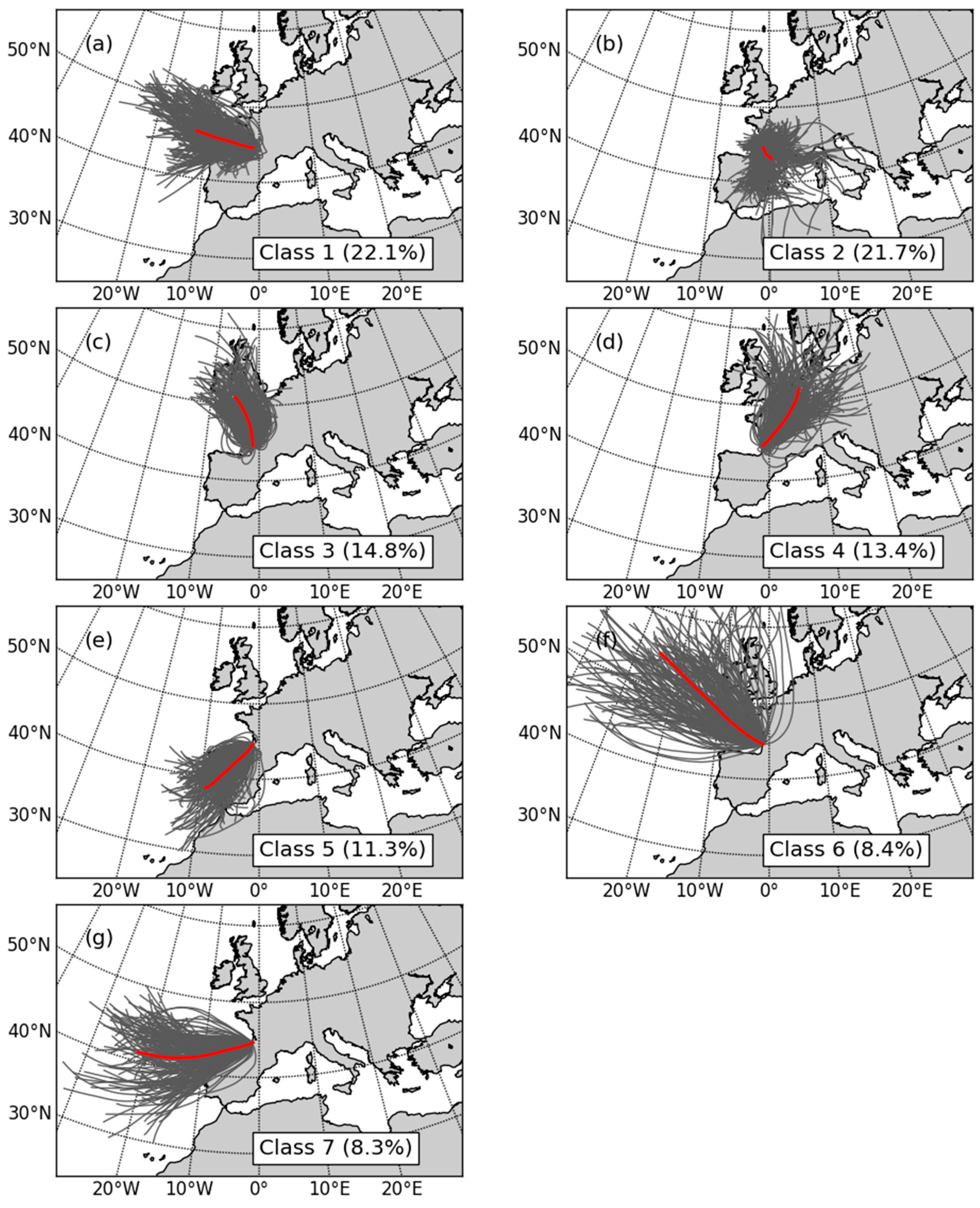
3.2. Identification of the Aerosol Origin at Synoptic Scale

In order to investigate the origin of the aerosols found at the Arcachon lagoon due to long-range transport, a nonhierarchical cluster analysis is applied to calculate the three-day back trajectories by means of the NOAA hybrid single-particle Lagrangian integrated trajectory (HYSPLIT) model. The cluster analysis allows us to group together the back-trajectories with similar lengths, indicating the wind speed, and curvature. Based on this statistical grouping method, seven distinct classes of back trajectories can be identified (Figure 7). As in Toledano et al. [82], classes characterized by a mean wind direction and speed are referred to by the following numerical labels: west (class 1), slow southeast (2), north–northwest (3), north–northeast (4), southwest (5), fast northwest (6), and fast west–southwest (7).
Figure 7 shows that the classes 1, 3, 6 and 7 are mainly associated with Atlantic air masses and comprise 53.6% of the back trajectories cases. Classes 2, 4 and 5 primarily include the continental air masses and correspond to 46.4% of the cases. The seasonal distribution of the trajectory occurrences for each class is given in Figure 8. Classes 6 and 7 associated with a high wind speed (longer trajectory length) show the highest trajectory occurrence values during the months of fall and winter (77% and 72% of cases, respectively), while class 2 associated with low wind speed (shorter trajectory length) is characterized by the highest occurrence value in spring and summer (66%). Combining the percentage of air mass back trajectories (Figure 7) and the seasonal frequency of trajectory occurrences (Figure 8) associated with each class, we show that the back trajectories in spring and summer are mainly represented by classes 1 and 2 (56.3% of cases), while only 8.4% of occurrences are associated with classes 6 and 7. For the months of fall and winter, the class-membership distribution is more balanced with a maximum value of 16.8% (class 1) and a minimum value of 12% (class 7).
Table 3 presents the mean values of the aerosol properties and the proportion of the different aerosol types associated with the seven classes. The calculation of these parameters is restricted to only the days for which there are valid CIMEL measurements. Atlantic air masses (classes 1, 3, 6 and 7) present low mean values of AOD, α 440 870 , and FMF. The lowest mean values are associated with long-range transport from the northwest (class 6) and west-southwest (class 7), which also occur primarily during fall and winter when storm winds are the strongest [84,85]. The mean AOD is 0.09. The mean α 440 870 are 0.52 and 0.77, while the mean FMF are 36% and 48%, respectively. These values indicate the dominant presence of marine aerosol as highlighted by the high proportion of CM type aerosols (52% and 53%). This was also associated with a high proportion of MM type aerosols (40% and 30%). Classes 1 and 3 associated with transport of air masses occurring mainly in spring and summer show moderately low mean values compared to the total means calculated over the whole data set (Table 2). However, the proportions of CM type aerosols (27% and 29%, respectively) are still high compared to the total mean (17%, Table 2). The proportion of the BU and DU types are more balanced, which indicates that aerosols have a predominantly marine origin combined with continental components.
Continental air masses (classes 2, 4 and 5) present high mean values of AOD, α 440 870 and FMF. The highest mean value of AOD (0.20) is associated with short trajectories (class 2) occurring primarily during spring and summer, which indicates local sources of aerosols. In comparison, the highest values of α 440 870 and FMF (1.36 and 74%) are observed for the class 4 characterized by a longer air mass transport, which originates from central and northern Europe. Although the origin of aerosols is considerably different, the proportions of the different aerosol types are similar, especially with a high proportion of the BU type (26% and 28%, respectively). The main exception is the proportion of the DU type (7% and 2%), which indicates that there is a significant component of Saharan dust in the class 2 aerosols. Saharan dust associated with North African air masses are also transported by the southwesterly trajectories (class 5), which present the highest proportion of the DU type (8%).

3.3. Development of a Regional Aerosol Model (RAM)

In this study, the approach used to define a regional atmospheric aerosol particle model (RAM) is based on the analysis of the temporal variability of the aerosol types as well as their associated optical and microphysical properties. These properties are derived from an analysis of the aerosol climatology. Analyses clearly demonstrate that the most representative situation is characterized by the presence of mixed-type aerosols originating from Atlantic Ocean (Figure 7), which also show a bimodal PSD regardless of the season (Figure 6). This result allows for the reasonable assumption that aerosol properties over the Arcachon lagoon can be modeled by the spectral mixture of two distinct monomodal distributions associated with a fine and coarse mode, respectively. The fine mode is associated with continental aerosols, while the coarse mode is associated with oceanic aerosols. Considering that oceanic aerosols are mostly composed of non-absorbing sea-salt particles, we further assume that any absorption of light propagating through the atmosphere is due to the fine mode aerosol particles. This assumption is not completely true, in particular when aerosols are composed of urban/industrial and desert dust particles. However, the probability of this occurrence is low (Table 3) and we believe that this assumption is realistic.
Because of the lack of in-situ data regarding the optical and chemical composition of atmospheric aerosol particles, we propose a simplified version of the RAM based on the classification of Shettle and Fenn [62]. The continental aerosols of the fine mode and oceanic aerosols of the coarse mode are associated with the tropospheric and maritime aerosol models, respectively. The maritime aerosol model is composed of sea salts (95%) and water-soluble (5%) particles, while the tropospheric model consists of a mixture of 70% of water-soluble substances (ammonium, calcium sulfate, and organic compounds) and 30% of dust-like particles. The RAM is intended to represent the general aerosol conditions in the study area, which is supposed to not be directly impacted by urban and/or industrial aerosol sources (mainly represented by class 2). Based on the results displayed in Figure 7, the RAM should be relevant in approximately 70% of the different weather regimes (roughly all classes except class 2 and 4).
It is important to note that the aerosol models of Shettle and Fenn [62] are hygroscopic, which indicate that the microphysical properties of the aerosols depend on the relative humidity. Those effects were integrated in the RAM following the method described by Ahmad et al. [38]. The growth of the volume geometric mean radius ( r v i ) as a function of Rh has been compared with the Arcachon AERONET data [66]. There was consistency for the fine mode, while a high overestimation has been shown for the coarse mode. Bru [66] demonstrated that the overestimation is directly related to the correction of the volume geometric mean radius of coarse particles ( r v c ) proposed by Ahmad et al. [38]. The correction of Ahmad et al. [38] consists to increase r v c by a factor of 3 σ c (the standard deviation of the monthly mean of the coarse-mode AERONET data) in order to ensure that their models of the oceanic aerosol size distribution spanned the full range of the satellite observations. For the coastal site of Arcachon, Bru [66] shown that this correction introduces a bias for the r v c retrievals. When the correction is not applied, the r v c model matches well with the AERONET data. Therefore, we decided to not apply this correction in this study. Following this, the optical properties were derived from the formulations of Shettle and Fenn [62]. The values of the modal radii and standard deviations for fine and coarse modes as well as the complex refractive index associated with the RAM for different values of Rh are provided by Bru [66].
This first version of the RAM relies on a compromise between the need for a flexible and robust model, which allows for processing of a huge number of satellite images associated with a wide range of maritime and tropospheric aerosols. Following this, the main limitation is currently due to the fact that absorbing aerosols are only partially taken into account. The effects of the radiation absorption by aerosols are crucial for the accuracy of the water-leaving reflectance retrievals as explained in Bassani et al. [39]. To improve the performance of the SACOR approach, an analysis of the variability of the single scattering albedo and the imagery part of the refractive index of the atmospheric particles should be performed in order to classify the absorbing aerosol types and integrate them into the RAM.

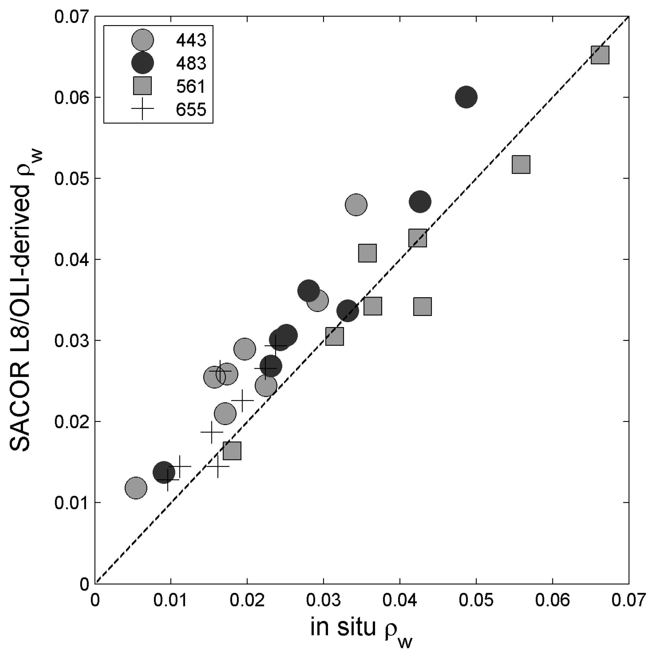
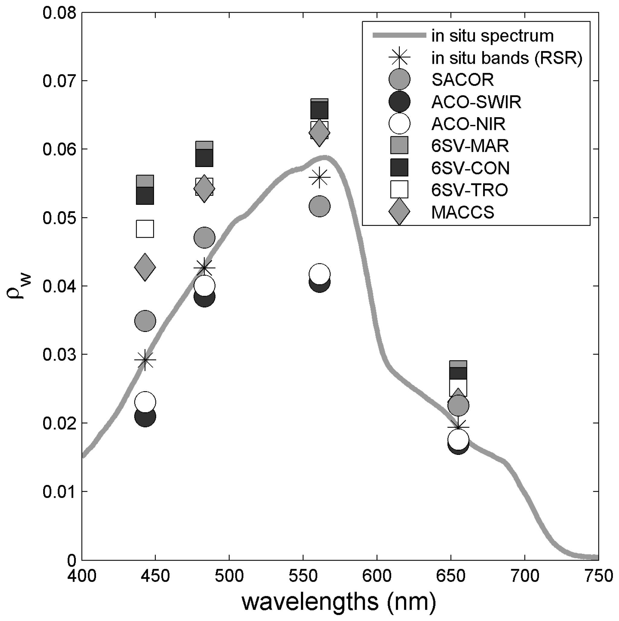
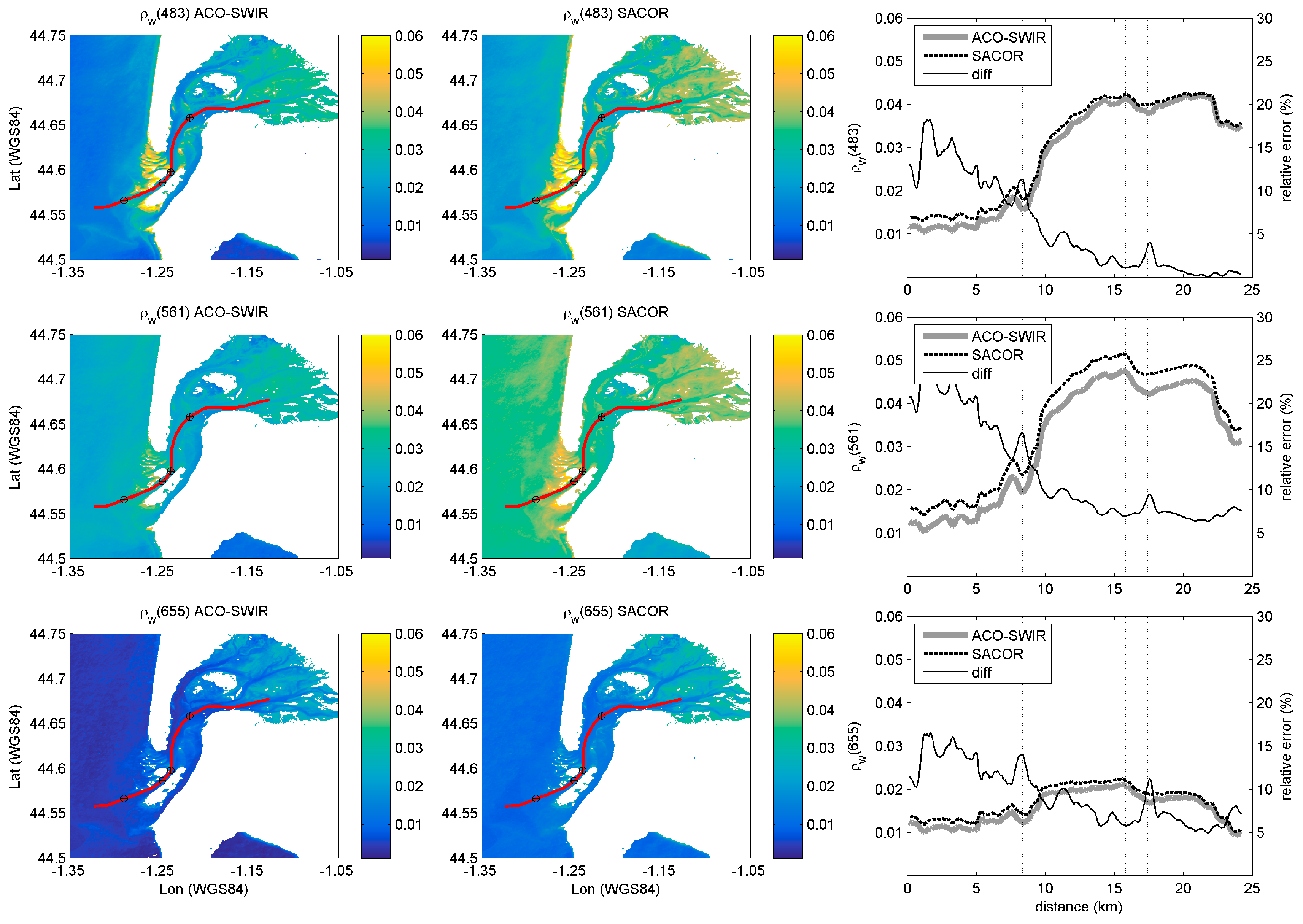
3.4. Assessment of SACOR Performances

The SACOR, ACO-SWIR, ACO-NIR, 6SV-MAR, 6SV-CON, and 6SV-TRO atmospheric corrections were applied to the Level 1T OLI data listed in Table 1 for inter-comparison and validation using in situ-measured water-leaving reflectance. Atmospheric inputs used in SACOR and 6SV were constrained by the AERONET and meteorological station data (Table 1). The downloaded MACCS atmospherically corrected products provided by the Theia Data Center were already processed. As described in Section 2.4.2, evaluation of the SACOR performances follows a two-step process based on match-up and inter-comparison exercises.
Figure 9 shows the comparison between ρ w derived from the SACOR atmospheric corrections and recorded from in-situ measurements at the four visible spectral bands of OLI. The values of the overall coefficient of determination (r2 = 0.90) and regression parameters (slope = 0.89 and intercept = 0.002) for the match-up sets indicate good performances of SACOR for deriving the magnitude and the spectral shape of ρ w . The overall relative error is approximately 24% (Table 4). The lowest error is observed for the green channel (561 nm) with a value of 7%, while the highest error (46%) is observed for the coastal channel (443 nm). Furthermore, ρ w presents a relative error of 21% and 22% for the blue (483 nm) and red (655 nm) channels, respectively. It is important to note that the large overestimation observed in the coastal band is well known [32]. In particular, Pahlevan et al. [86] shown that the OLI-derived reflectances are brighter at 443 nm than retrievals of standard ocean color missions.
Figure 10 provides an example of the ρ w values estimated from OLI data, which were atmospherically corrected from SACOR and computed from the RSR-adjusted in-situ measurements for 20 October, 2015. For comparison, the products provided by the other atmospheric corrections are also reported on Figure 10. It is important to note that the other match-ups show similar trends. When SACOR is used to process OLI data, a low overestimation of ρ w is observed at the coastal, blue and red bands, while a low underestimation is found at the green band. ACO-SWIR and ACO-NIR show an underestimation of ρ w regardless of the channel, with the highest error occurring at the green channel. For this match-up, the lowest performances are observed for 6SV-MAR, -CON, -TRO as well as MACCS with a high overestimation of ρ w regardless of the channel. This result highlights the need to correctly estimate both the particle modal radii size which depends on Rh, and the aerosol type to accurately derive the water-leaving reflectance.
Table 4 provides the relative error between the satellite-derived and measured ρ w , which is computed from the eight match-ups. ACO-SWIR shows the best overall performance with a mean relative error of 19%. ACO-SWIR outperforms SACOR for the coastal, blue and red channels (21% and 46%; 13% and 21%; 14% and 22%, respectively). There is an exception for the green channel (27% versus 7%), where a significant underestimation is observed. The origin of this underestimation already reported by Vanhellemont et al. [13] and Novoa et al. [69] is still unclear. The other atmospheric corrections show a significantly lower performance compared to ACO-SWIR and SACOR. In particular, the differences observed in the ρ w estimates from 6SV-MAR, -CON and -TRO highlight the importance of the aerosol model. In general, a high overestimation of the ρ w values is observed regardless of the channels, as illustrated in Figure 10. These errors can be directly attributed to the use of an inaccurate aerosol model, which provides an underestimation of the atmospheric component.
Figure 11 shows the ρ w estimates obtained from ACO-SWIR and SACOR in the OLI coastal, blue, green and red bands over the Arcachon lagoon and the adjacent coastal zone for 20 October, 2015. The ρ w maps provided by ACO-SWIR and SACOR show similar patterns associated with a low noise level, which is probably due to the low sea-surface roughness (wind speed < 1 m/s). The normalized environmental noise equivalent water-leaving reflectance difference (NNE∆ ρ w ) is computed for each image following the methodology of Wettle et al. [87] and using the normalized root mean square error (NRMSE) [69]. To quantify NNE∆ ρ w , a box of 50 × 50 pixels is extracted from an optically homogeneous area, which is located far from the coastal plume. The results indicate a similar noise level between the atmospheric correction methods with a NNE∆ ρ w value of 3.4% (4.7%), 3.9% (3.9%) and 5.8% (6.5%) for ACO-SWIR (SACOR) at the blue, green and red bands, respectively. This highlights the consistent between the ρ w estimates and the reliability of SACOR. These performances are strengthened by the good correlation observed between the ρ w estimates obtained from ACO-SWIR and SACOR along the cross-shore transection.
However, the relative differences between the two atmospheric correction methods are significant with a mean value of 5.9%, 12.3% and 9.4% at 483 nm, 561 nm and 655 nm, respectively. SACOR causes the water-leaving reflectance values to be higher than the values obtained from ACO-SWIR. Furthermore, the difference between the values is significantly higher in the inner part of the Arcachon lagoon compared to the outer part of the inlet.
The relative difference is clearly correlated with bio-optical changes along the cross-shore transection, which is represented on Figure 11 by vertical dashed lines and black plus-sign circle symbols. The highest relative difference is found between the Point kilometer 0 (PK0) and PK8.4, where the optical properties of the sea-water are dominated by the particles and dissolved matter coming from rivers and internal channels of the lagoon. Beyond PK8.4, where the sea-water is optically influenced by the coastal ocean, the relative difference decreases and becomes non-significant with respect to the NNE∆ ρ w at 483 nm and 655 nm. It is important to note that, between PK8.4 and PK22.1, the bottom can influence the ρ w spectrum due to a lesser water depth associated with a low diffuse attenuation coefficient [12]. For example, a maximum ρ w estimated value is observed at PK15.8 and PK22.1, where the bathymetry values are −7.1 and −8.6 m, respectively. The minimum value observed at PK17.4 is associated with a bathymetry of −11.3 m.
However, the hypothesis of a causal relationship between the relative difference and sea-water optical properties is unlikely as ACO-SWIR and SACOR make no assumption on the spectral shape of ρ w . To explain this result, two other reasons have to be considered, which are namely: (1) the non-homogeneity of the aerosol spatial distribution over the scene and (2) the presence of the absorbing urban aerosol associated with the mixed continental type (Table 1). Match-ups are generally associated with meteorological windows characterized by a low wind speed (<1 m/s), which generates a low horizontal transport favorable for a spatial aerosol gradient. This gradient may be schematically characterized by a continental aerosol pool within the inner part of the lagoon and a maritime aerosol pool within the outer part of the inlet. In this case, the difference between the ρ w estimated values could be lower in the inner than in the outer part of the lagoon. For ACO-SWIR, the overrepresentation of the offshore waters should lead to the application of a sub-tile fixed epsilon that is more representative of the maritime aerosol model and consequently, underestimates ρ a (overestimate ρ w ) in the inner part of the lagoon. For SACOR, the aerosol model is defined by the in-situ parameters provided by the CIMEL station located in the inner part of the lagoon. Consequently, the aerosol model applied for the whole scene should be more representative of the continental aerosol model and leads to an overestimation of ρ a (underestimation of ρ w ) in the outer part of the lagoon and in the inner part of the lagoon due to an underestimation of absorbing aerosols.

4. Conclusions

In this paper, we present the first developments of an atmospheric correction (AC) method dedicated to the processing of high spatial resolution space mission data for littoral applications. The in Situ-based Atmospheric CORrection (SACOR) algorithm is based on atmospheric radiative transfer simulations using the Successive Order of Scattering code (SOS) and a regional aerosol model (RAM). Thus, the first objective of the study was to define a RAM for the site of Arcachon (France), using both: (i) a 6-year time series of aerosol optical and microphysical properties acquired through the ground-based PHOTONS/AERONET network; and (ii) a 6-year aerosol climatology using the NOAA hybrid single-particle Lagrangian integrated trajectory (HYSPLIT) model. The second objective was to validate the SACOR water-leaving reflectance ( ρ w ) retrievals using field measurements and to inter-compare the performances of the method using standard AC algorithms.
To characterize an appropriate RAM for the study site of Arcachon, we examined the seasonal behavior of aerosol microphysical and optical properties using a few selected mean daily parameters, including the aerosol optical depth at 500 nm (AOD), the Ångström coefficient computed between 440 and 870 nm ( α 440 870 ), the aerosol particle size distribution (PSD), and the AOD fine mode fraction (FMF). Analysis of the mean geometric modal radius and standard deviation time series was initially performed by Bru [66]. Results show a significant seasonal variability of these parameters. In particular, the analysis of the α 440 870 , PSD and FMF time series shows that there are finer atmospheric particles in spring and summer than in fall and winter, with an inverse pattern found for coarse aerosols. The study of the variability of aerosol types, identified using a classification based on the α 440 870 -AOD scatter plot, shows that the maritime type (composed of clean maritime and mixed maritime aerosols) represents 31% of occurences. The highest proportion occurs in fall and winter. The biomass burning/urban-industrial and dust particle types represent 19% of occurences and show a maximum proportion in spring and summer. However, the main results for defining a suitable RAM are characterized by PSD having a bimodal distribution and aerosols being primarily dominated by the coastal continental type regardless of the season. This indicates aerosols of very varied origin, which is consistent with the results of Smirnov et al. [35] for the North Atlantic sites. The results of the aerosol classification are then validated using a climatological study, which confirms that the aerosol origin is maritime first, followed by continental and local. These observations allow for a reasonable assumption that aerosol properties over the Arcachon lagoon can be modeled by the spectral mixture of two distinct monomodal distributions associated with a fine (coarse) mode and a tropospheric (maritime) aerosol model, as defined by Shettle and Fenn [62].
The performances of the SACOR method are evaluated using Landsat-8/Operational Land Imager (OLI) images acquired over the Arcachon lagoon and processed using AERONET (AOD, FMF, and water vapor) and meteorological data ( R h ). The validation and inter-comparison exercises are performed using in-situ ρ w measurements and atmospherically corrected OLI products computed using the standard AC models. The results show consistency between SACOR-derived and in-situ ρ w with an overall relative error (RE) of 24% for visible spectral bands. SACOR shows the best performance at green wavelengths (RE of 7%) compared to the other AC methods. However, for the other visible channels, the SWIR-based ACOLITE (ACO-SWIR) method provides better results. The impact of the aerosol model on ρ w retrievals is clearly demonstrated. The atmospherically corrected products provided by MACCS and the 6SV simulations using the different standard aerosol models (continental, maritime, and tropospheric) show a large overestimation of ρ w . The lower value of the particle modal radii size (at the dry state) used by the 6S models may partially explain this result. The forward scattering of small atmospheric particles is higher than large particles. Finally, the comparison of ρ w retrievals between ACO-SWIR and SACOR along a cross-shore transection demonstrates the robustness of our methodology. Furthermore, the analysis of relative differences along the transection allows highlighting the limit of the assumptions about the homogeneity of the aerosol spatial distribution over the scene and the absence of absorbing urban aerosol in the RAM.
The good results obtained in this study demonstrate the relevance of the SACOR method. SACOR is an innovative approach to process HRS space mission data without information at the NIR and SWIR wavelengths (such as SPOT and Pleiades) for littoral applications. Additionally, SACOR is an alternative AC method for decametric space missions (Landsat-8, Sentinel-2) and provides ρ w retrievals for regional intercomparison exercises with standard AC models [88]. The SACOR method developed in this paper should be considered as a first version due to the simplified RAM proposed by authors. As previously reported, the simplified aerosol model can be problematic for the processing of some satellite scenes associated with specific meteorological conditions for which atmospheric particles may be dominated by dust or absorbing urban-industrial particles. A non-absorbing aerosol model can lead to a significant over-correction of the top-of-atmosphere signal in the blue bands, which could generate negative ρ w values [89]. Another potential limit of the RAM is the use of AERONET monthly mean values of modal radii and standard deviation for SOS simulations, which can generate errors for ρ w retrievals in the blue-green channels as demonstrated by Ahmad et al. [38]. To address some of those issues, an accurate analysis of the optical and chemical properties of aerosols over the Arcachon lagoon is needed. Future steps will concern the development of specific regional aerosol models for each weather regime and the integration of up-to-date knowledge on aerosol microphysical and optical properties based on in-situ measurements into these models. This should be pursued in order to develop an adaptive aerosol model function of the origin of atmospheric air masses.

Acknowledgments

This work was supported by the Centre National d’Etude Spatiale (CNES) in the framework of the MORITO and BIM projects (TOSCA program). We are grateful to the crew of the Planula IV (CNRS/INSU). USGS and NASA are acknowledged for the Landsat-8/OLI images. The authors would also like to thank the CESBIO and CNES for providing MACCS-corrected Landsat-8/OLI data on the Theia web portal. We thank the French National Observatory Network for Aerosol (PHOTONS) and Aerosol Robotic Network (AERONET) staffs for maintaining and providing the sunphotometer data used in this study. In addition, we are grateful to METEO-FRANCE and OASU for providing meteorological data. We thank three anonymous reviewers for helpful comments.

Author Contributions

Driss Bru developed the SACOR algorithm. Driss Bru, Cassandra Normandin and Arthur Robinet provided atmospherically-corrected OLI images using SACOR, 6SV and ACOLITE methods. Olivier Hagolle provided atmospherically-corrected OLI images using MACCS algorithm. Bertrand Lubac provided field radiometric data. Michel Leconte and Nadège Martiny provided AERONET data. Driss Bru and Bertrand Lubac analyzed the data and wrote the paper. Cédric Jamet, Nadège Martiny and Olivier Hagolle contributed interpreting results and writting the paper.

Conflicts of Interest

The authors declare no conflict of interest. The founding sponsors had no role in the design of the study; in the collection, analyses, or interpretation of data; in the writing of the manuscript, and in the decision to publish the results.

References

  1. Newton, A.; Weichselgartner, J. Hotspots of coastal vulnerability: A DPSIR analysis to find societal pathways and responses. Estuar. Coast. Shelf Sci. 2014, 140, 123–133. [Google Scholar] [CrossRef]
  2. Nicholls, R.J. Planning for the impacts of sea level rise. Oceanography 2011, 24, 144–157. [Google Scholar] [CrossRef]
  3. Nicholls, R.J.; Wong, P.P.; Burkett, V.R.; Woodroffe, C.D.; Hay, J.E. Climate change and coastal vulnerability assessment: Scenarios for integrated assessment. Sustain. Sci. 2008, 3, 89–102. [Google Scholar] [CrossRef]
  4. Burkett, V.R.; Davidson, M.A. Coastal Impacts, Adaptation and Vulnerability: A Technical Input to the 2013 National Climate Assessment; Burkett, V.R., Davidson, M.A., Eds.; Island Press: Washington, DC, USA, 2012; p. 188. ISBN 978-1610914604. [Google Scholar]
  5. Le Treut, H. Les impacts du changement climatique en Aquitaine: Etat des lieux scientifique; Presses Universitaires de Bordeaux Pessac: Pessac, France, 2013. [Google Scholar]
  6. International Ocean-Colour Coordinating Group. Why Ocean Colour? The Societal Benefits of Ocean-Colour Technology; Platt, T., Hoepffner, N., Stuart, V., Brown, C., Eds.; International Ocean-Colour Coordinating Group: Dartmouth, NS, Canada, 2008. [Google Scholar]
  7. International Ocean-Colour Coordinating Group. Mission Requirements for Future Ocean-Colour Sensors; McClain, C.R., Meister, G., Eds.; International Ocean-Colour Coordinating Group: Dartmouth, NS, Canada, 2012. [Google Scholar]
  8. Klemas, V. Airborne remote sensing of coastal features and processes: An overview. J. Coastal. Res. 2013, 29, 239–255. [Google Scholar] [CrossRef]
  9. Mouw, C.B.; Greb, S.; Aurin, D.; DiGiacomo, P.M.; Lee, Z.; Twardowski, M.; Binding, C.; Hu, C.; Ma, R.; Moore, T.; et al. Aquatic color radiometry remote sensing of coastal and inland waters: Challenges and recommendations for future satellite missions. Remote Sens. Environ. 2015, 160, 15–30. [Google Scholar] [CrossRef]
  10. Pahlevan, N.; Lee, Z.; Hu, C.; Schott, J.R. Diurnal remote sensing of coastal/oceanic waters: A radiometric analysis for geostationary coastal and air pollution events. Appl. Opt. 2014, 53, 648–665. [Google Scholar] [CrossRef] [PubMed]
  11. Roy, D.P.; Wulder, M.A.; Loveland, T.R.; Woodcock, C.E.; Allen, R.G.; Anderson, M.C.; Helder, D.; Irons, J.R.; Johnson, D.M.; Kennedy, R.; et al. Landsat-8: Science and product vision for terrestrial global change research. Remote Sens. Environ. 2014, 145, 154–172. [Google Scholar] [CrossRef]
  12. Capo, S.; Lubac, B.; Marieu, V.; Robinet, A.; Bru, D.; Bonneton, P. Assessment of the decadal morphodynamic evolution of a mixed energy inlet using ocean color remote sensing. Ocean Dyn. 2014, 64, 1517–1530. [Google Scholar] [CrossRef]
  13. Vanhellemont, Q.; Ruddick, K. Turbid wakes associated with offshore wind turbines observed with Landsat 8. Remote Sens. Environ. 2014, 145, 105–115. [Google Scholar] [CrossRef]
  14. Hagolle, O.; Huc, M.; Pascual, D.V.; Dedieu, G. A multi-temporal and multi-spectral method to estimate aerosol thickness over land, for the atmospheric correction of Formosat-2, LandSat, VENμs, and Sentinel-2 images. Remote Sens. 2015, 7, 2668–2691. [Google Scholar] [CrossRef]
  15. Gordon, H.R.; Wang, M. Retrieval of water-leaving radiance and aerosol optical thickness over the oceans with SeaWIFS: A preliminary algorithm. Appl. Opt. 1994, 33, 443–452. [Google Scholar] [CrossRef] [PubMed]
  16. Ruddick, K.; Ovidio, F.; Rijkeboer, M. Atmospheric correction of SeaWIFS imagery for turbid coastal and inland waters. Appl. Opt. 2000, 39, 897–912. [Google Scholar] [CrossRef] [PubMed]
  17. Wang, M.; Shi, W. Estimation of ocean contribution at the MODIS near-infrared wavelengths along the east coast of the U.S.: Two case studies. Geophys. Res. Lett. 2005, 32, L13606. [Google Scholar] [CrossRef]
  18. Jamet, C.; Loisel, H.; Kuchinke, C.P.; Ruddick, K.; Zibordi, G.; Feng, H. Comparison of three SeaWIFS atmospheric correction algorithms for turbid waters using AERONET-OC measurements. Remote Sens. Environ. 2011, 115, 1955–1965. [Google Scholar] [CrossRef]
  19. Vanhellemont, Q.; Ruddick, K. Advantages of high quality SWIR bands for ocean colour processing: Examples from Landsat-8. Remote Sens. Environ. 2015, 161, 89–106. [Google Scholar] [CrossRef]
  20. Wang, M. Remote sensing of the ocean contributions from ultraviolet to nearinfrared using the shortwave infrared bands: Simulations. Appl. Opt. 2007, 46, 1535–1547. [Google Scholar] [CrossRef] [PubMed]
  21. He, X.; Bai, Y.; Pan, D.; Huang, N.; Dong, X.; Chen, J.; Chen, C.-T.A.; Cui, Q. Using geostationary satellite ocean color data to map the diurnal dynamics of suspended particulate matter in coastal waters. Remote Sens. Environ. 2013, 133, 225–239. [Google Scholar] [CrossRef]
  22. Hu, C.; Carder, K.L.; Muller-Karger, F.E. Atmospheric correction of SeaWIFS imagery over turbid coastal waters. Remote Sens. Environ. 2000, 74, 195–206. [Google Scholar] [CrossRef]
  23. Shanmugan, P.; Ahn, Y. New atmospheric correction technique to retrieve the ocean colour from SeaWiFS imagery in complex coastal waters. J. Opt. A Pure Appl. Opt. 2007, 9, 511–530. [Google Scholar] [CrossRef]
  24. Kuchinke, C.P.; Gordon, H.R.; Franz, B.A. Spectral optimization for constituent retrieval in Case II waters I: Implementation and performance. Remote Sens. Environ. 2009, 13, 571–587. [Google Scholar] [CrossRef]
  25. Kuchinke, C.P.; Gordon, H.R.; Harding, L.W., Jr.; Voss, K.J. Spectral optimization for constituent retrieval in Case II waters II: Validation study in the Chesapeake Bay. Remote Sens. Environ. 2009, 113, 610–621. [Google Scholar] [CrossRef]
  26. Brajard, J.; Santer, R.; Crépon, M.; Thiria, S. Atmospheric correction of MERIS data for case-2 waters using a neuro-variational inversion. Remote Sens. Environ. 2012, 126, 51–61. [Google Scholar] [CrossRef]
  27. Doerffer, R.; Schiller, H. The MERIS Case 2 algorithm. Int. J. Remote Sens. 2007, 28, 517–535. [Google Scholar] [CrossRef]
  28. Schroeder, T.; Behnert, I.; Schaale, M.; Fischer, J.; Doerffer, R. Atmospheric correction algorithm for MERIS above case-2 waters. Int. J. Remote Sens. 2007, 28, 1469–1486. [Google Scholar] [CrossRef]
  29. Stumpf, R.P.; Arnone, R.A.; Gould, R.W.; Ransibrahmanakul, V. A partly coupled ocean-atmosphere model for retrieval of water-leaving radiance from SeaWIFS in coastal waters. NASA Tech. Memo. 2003, 206892, 51–59. [Google Scholar]
  30. Bailey, S.W.; Franz, B.A.; Werdell, P.J. Estimation of near-infrared water-leaving reflectance for satellite ocean color data processing. Opt. Express 2010, 18, 7521–7527. [Google Scholar] [CrossRef] [PubMed]
  31. Goyens, C.; Jamet, C.; Ruddick, K.G. Spectral relationships for atmospheric correction. I. Validation of red and near infra-red marine reflectance relationships. Opt. Express 2013, 21, 21162–21175. [Google Scholar] [CrossRef] [PubMed]
  32. Goyens, C.; Jamet, C.; Ruddick, K.G. Spectral relationships for atmospheric correction. II. Improving NASA's standard and MUMM near infra-red modeling schemes. Opt. Express 2013, 21, 21176–21187. [Google Scholar] [CrossRef] [PubMed]
  33. Wang, M.; Shi, W.; Jiang, L. Atmospheric correction using near-infrared bands for satellite ocean color data processing in the turbid western pacific region. Opt. Express 2012, 20, 741–753. [Google Scholar] [CrossRef] [PubMed]
  34. Jiang, L.; Wang, M. Improved near-infrared ocean reflectance correction algorithm for satellite ocean color data processing. Opt. Express 2014, 22, 21657–21678. [Google Scholar] [CrossRef] [PubMed]
  35. Smirnov, A.; Holben, B.; Kaufman, Y.J.; Dubovik, O.; Eck, T.F.; Slutsker, I.; Pietras, C.; Halthore, R.N. Optical properties of atmospheric aerosol in marine environments. J. Atmos. Sci. 2002, 59, 501–523. [Google Scholar] [CrossRef]
  36. Dubovik, O.; Holben, B.; Eck, T.F.; Smirnov, A.; Kaufman, Y.J.; King, M.D.; Tanre, D.; Slutsker, I. Variability of absorption and optical properties of key aerosol types observed in worldwide locations. J. Atmos. Sci. 2002, 59, 590–608. [Google Scholar] [CrossRef]
  37. Martiny, N.; Frouin, R.; Santer, R. Radiometric calibration of SeaWIFS in the near infrared. Appl. Opt. 2005, 44. [Google Scholar] [CrossRef]
  38. Ahmad, Z.; Franz, B.A.; McClain, C.R.; Kwiatkowska, E.J.; Werdell, J.; Shettle, E.P.; Holben, B.N. New aerosol models for the retrieval of aerosol optical thickness and normalized water-leaving radiances from the SeaWiFS and MODIS sensors over coastal regions and open oceans. Appl. Opt. 2010, 49, 5545–5560. [Google Scholar] [CrossRef] [PubMed]
  39. Bassani, C.; Manzo, C.; Braga, F.; Bresciani, M.; Giardino, C.; Alberotanza, L. The impact of the microphysical properties of aerosol on the atmospheric correction of hyperspectral data in coastal waters. Atmos. Meas. Tech. 2015, 8, 1593–1604. [Google Scholar] [CrossRef]
  40. Vermote, E.; Justice, C.; Claverie, M.; Franch, B. Preliminary analysis of the performance of the Landsat 8/OLI land surface reflectance product. Remote Sens. Environ. 2016, 185, 46–56. [Google Scholar] [CrossRef]
  41. Glé, C.; Del Almo, Y.; Sautour, B.; Labore, P.; Chardy, P. Variability of nutrients and phytoplankton primary production in a shallow macrotidal coastal ecosystem (Arcachon Bay, France). Estuar. Coast. Shelf Sci. 2008, 76, 642–656. [Google Scholar] [CrossRef]
  42. Dubois, S.; Savoye, N.; Gremare, A.; Plus, M.; Charlier, K.; Beltoise, A.; Blanchet, H. Origin and composition of sediment organic matter in a coastal semi-enclosed ecosystem: An elemental and isotopic study at the ecosystem space scale. J. Mar. Syst. 2012, 94, 64–73. [Google Scholar] [CrossRef]
  43. Polsenaere, P.; Abril, G. Modelling CO2 degassing from small acidic rivers using water pCO2, DIC and δ13C-DIC data. Geochim. Cosmochim. Acta 2012, 91, 220–239. [Google Scholar] [CrossRef]
  44. Puillat, I.; Lazure, P.; Jégou, A.-M.; Lampert, L.; Miller, P. Mesoscale hydrological variablity induced by northwesterly wind on the French continental shelf of the Bay of Biscay. Sci. Mar. 2006, 70, 15–26. [Google Scholar] [CrossRef]
  45. Robinet, A.; Castelle, B.; Idier, D.; Le Cozannet, G.; Déqué, M.; Charles, E. Statistical modeling of interannual shoreline change driven by north Atlantic climate variability spanning 2000–2014 in the Bay of Biscay. Geo-Mar. Lett. 2016, 36, 479–490. [Google Scholar] [CrossRef] [Green Version]
  46. LA QUALITÉ DE L’AIR EN NOUVELLE-AQUITAINE AIRAQ. Available online: http://www.atmo-nouvelleaquitaine.org/publications/bilan-des-donnees-aquitaine-2015 (accessed on 7 March 2016).
  47. Dubovik, O.; King, M.D. A flexible inversion algorithm for retrieval of aerosol optical properties from Sun and sky radiance measurements. J. Geophys. Res. 2000, 105, 20673–20696. [Google Scholar] [CrossRef]
  48. Holben, B.N.; Eck, T.F.; Slutsker, I.; Tanré, D.; Buis, J.P.; Setzer, A.; Vermote, E.; Reagan, J.A.; Kaufman, Y.; Nakajima, T.; et al. AERONET—A federated instrument network and data archive for aerosol characterization. Remote Sens. Environ. 1998, 66, 1–16. [Google Scholar] [CrossRef]
  49. Holben, B.N.; Tanré, D.; Smirnov, A.; Eck, T.F.; Slutsker, I.; Abuhassan, N.; Newcomb, W.W.; Schafer, J.; Chatenet, B.; Lavenue, F.; et al. An emerging ground-based aerosol climatology: Aerosol optical depth from AERONET. J. Geophys. Res. 2001, 106, 12067–12097. [Google Scholar] [CrossRef]
  50. O’Neill, N.T.; Eck, T.F.; Smirnov, A.; Holben, B.N.; Thulasiraman, S. Spectral discrimination of coarse and fine mode optical depth. J. Geophys. Res. 2003, 108. [Google Scholar] [CrossRef]
  51. Draxler, R.R.; Hess, G.D. Description of the HYSPLIT_4 Modeling System. Available online: http://warn.arl.noaa.gov/documents/reports/arl-224.pdf (accessed on December 1997).
  52. Draxler, R.R. HYSPLIT4 User’s Guide. Available online: http://www.villasmunta.it/pdf/User_guide.pdf (accessed on June 1999).
  53. Stein, A.F.; Draxler, R.R.; Rolph, G.D.; Stunder, B.J.B.; Cohen, M.D.; Ngan, F. NOAA’s HYSPLIT atmospheric transport and dispersion modeling system. Bull. Am. Meteorol. Soc. 2015, 96, 2059–2077. [Google Scholar] [CrossRef]
  54. Toledano, C.; Cachorro, V.E.; De Frutos, A.M.; Torres, B.; Berjon, A.; Sorribas, M.; Stone, R.S. Airmass classification and analysis of aerosol types at El Arenosillo (Spain). J. Appl. Meteorol. Clim. 2009, 48. [Google Scholar] [CrossRef]
  55. Draxler, R.R.; Stunder, B.; Rolph, G.; Stein, A.; Taylor, A. HYSPLIT_4 User’s Guide; NOAA Air Resources Laboratory: Silver Spring, MD, USA, 2012. [Google Scholar]
  56. Draxler, R.R.; Stunder, B.; Rolph, G.; Stein, A.; Taylor, A. HYSPLIT Tutorial; NOAA Air Resources Laboratory: Silver Spring, MD, USA, 2012. [Google Scholar]
  57. Su, L.; Yuan, Z.; Fung, J.C.H.; Lau, A.K.H. A comparison of HYSPLIT backward trajectories generated from two GDAS datasets. Sci. Total Environ. 2015, 506, 527–537. [Google Scholar] [CrossRef] [PubMed]
  58. Gordon, H.R. Atmospheric correction of ocean color imagery in the Earth Observing System era. J. Geophys. Res. 1997, 102, 17081–17106. [Google Scholar] [CrossRef]
  59. Morel, A.; Gentili, G. Diffuse reflectance of oceanic waters. III. Implication of bidirectionality for the remote-sensing problem. Appl. Opt. 1996, 35, 4850–4862. [Google Scholar] [CrossRef] [PubMed]
  60. Frouin, R.; Pelletier, B. Bayesian methodology for inverting satellite ocean-color data. Remote Sens. Environ. 2015, 159, 332–360. [Google Scholar] [CrossRef]
  61. Hanel, G. The properties of atmospheric aerosol particles as functions of the relative humidity at thermodynamic equilibrium with the surrounding moist air. Adv. Geophys. 1976, 19, 73–188. [Google Scholar] [CrossRef]
  62. Shettle, E.P.; Fenn, R.W. Models for the Aerosols of the Lower Atmosphere and the Effects of Humidity Variations on Their Optical Properties. Available online: http://web.gps.caltech.edu/~vijay/Papers/Aerosol/SF79-Aerosol-Models-part1of4.PDF (accessed 20 September 1979).
  63. Deuzé, J.L.; Herman, M.; Santer, R. Fourier series expansion of the transfer equation in the atmosphere-ocean system. J. Quant. Spectrosc. Radiat. 1989, 41, 483–494. [Google Scholar] [CrossRef]
  64. Lenoble, J.; Herman, M.; Deuzé, J.L.; Lafrance, B.; Santer, R.; Tanré, D. A successive order of scattering code for solving the vector equation of transfer in the earth's atmosphere with aerosols. J. Quant. Spectrosc. Radiat. 2007, 107, 479–507. [Google Scholar] [CrossRef]
  65. Rahman, H.; Dedieu, G. SMAC: A simplified method for the atmospheric correction of satellite measurements in the solar spectrum. Int. J. Remote Sens. 1994, 15, 123–143. [Google Scholar] [CrossRef]
  66. Bru, D. Corrections atmosphériques pour capteurs à très haute résolution spatiale en zone littorale. Ph.D. Thesis, Univ. Bordeaux, Pessac, France, December 2015. [Google Scholar]
  67. Pahlevan, N.; Schott, J.R. Leveraging EO-1 to evaluate capability of new generation of landsat sensors for coastal/inland water studies. IEEE J. STARS 2013, 6, 360–374. [Google Scholar] [CrossRef]
  68. USGS. Available online: http://earthexplorer.usgs.gov/ (accessed on 31 July 2017).
  69. Novoa, S.; Doxaran, D.; Ody, A.; Vanhellemont, Q.; Lafon, V.; Lubac, B.; Gernez, P. Atmospheric corrections and multi-conditional algorithm for multi-sensor remote sensing of suspended particulate matter in low-to-high turbidity levels coastal waters. Remote Sens. 2017, 9. [Google Scholar] [CrossRef]
  70. Ruddick, K.; De Cauwer, V.; Park, Y.-J.; Moore, G. Seaborne measurements of near infrared water-leaving reflectance: The similarity spectrum for turbid waters. Limnol. Oceanogr. 2006, 51, 1167–1179. [Google Scholar] [CrossRef]
  71. Lubac, B.; Loisel, H. Variability and classification of remote sensing reflectance spectra in the eastern English Channel and southern North Sea. Remote Sens. Environ. 2007, 110, 45–58. [Google Scholar] [CrossRef]
  72. Vermote, E.; Tanré, D.; Deuzé, J.; Herman, M.; Morcrette, J.; Kotchenova, S. Second Simulation of a Satellite Signal in the Solar Spectrum-Vector (6SV); 6S User Guide Version; NASA Goddard Space Flight Center: Greenbelt, MD, USA, 2006. [Google Scholar]
  73. Theia. Available online: http://spirit.cnes.fr/resto/Landsat (accessed on January 2014).
  74. Hagolle, O.; Dedieu, G.; Mougenot, B.; Debaecker, V.; Duchemin, B.; Meygret, A. Correction of aerosol effects on multi-temporal images acquired with constant viewing angles: Application to Formosat-2 images. Remote Sens. Environ. 2008, 112, 1689–1701. [Google Scholar] [CrossRef] [Green Version]
  75. Kotchenova, A.Y.; Vermote, E.; Matarrese, R.; Klemm, F.J., Jr. Validation of a vector version of the 6S radiative transfer code for atmospheric correction of satellite data. Part I: Path radiance. Appl. Opt. 2006, 45, 6762–6774. [Google Scholar] [CrossRef] [PubMed]
  76. Barnaba, F.; Angelini, F.; Curci, G.; Gobbi, G.P. An important fingerprint of wildfires on the European aerosol load. Atmos. Chem. Phys. 2011, 11, 10487–10501. [Google Scholar] [CrossRef] [Green Version]
  77. Piazzola, J.; Forget, P.; Lafon, C.; Despiau, S. Spatial variation of sea-spray fluxes over a Mediterranean coastal zone using a sea-state model. Bound. Lay Meteorol. 2009, 132, 167–183. [Google Scholar] [CrossRef]
  78. Piazzola, J.; Tedeschi, G.; Demoisson, A. A model for the transport of sea-spray aerosols in the coastal zone. Bound. Lay Meteorol. 2015, 155, 329–350. [Google Scholar] [CrossRef]
  79. Pace, G.; Di Sarra, A.; Meloni, D.; Piacentino, S.; Chamard, P. Aerosol optical properties at Lampedusa (Central Mediterranean). 1. Influence of transport and identification of different aerosol types. Atmos. Chem. Phys. 2006, 6, 697–713. [Google Scholar] [CrossRef]
  80. Tan, F.; Lim, H.S.; Abdullah, K.; Yoon, T.L.; Holben, B. AERONET data-based determination of aerosol types. Atmos. Pollut. Res. 2015, 6, 682–695. [Google Scholar] [CrossRef]
  81. Lyamani, H.; Valenzuela, A.; Perez-Ramirez, D.; Toledano, C.; Granados-Munoz, M.J.; Olmo, F.J.; Alados-Arboledas, L. Aerosol properties over the western Mediterranean basin: Temporal and spatial variability. Atmos. Chem. Phys. 2015, 15, 2473–2486. [Google Scholar] [CrossRef]
  82. Toledano, C.; Sorribas, M.; Berjon, A.; De La Morena, B.A.; De Frutos, M.; Gouloub, P. Aerosol optical depth and Angstrom exponent climatology at El Arenosillo AERONET site (Huelva, Spain). Q. J. R. Meteorol. Soc. 2007, 133, 795–807. [Google Scholar] [CrossRef]
  83. Kaskaoutis, D.G.; Kambezidis, H.D.; Hatzianastassiou, N.; Kosmopoulos, P.G.; Badarinath, K.V.S. Aerosol climatology: On the discrimination of aerosol types over four AERONET sites. Atmos. Chem. Phys. Discuss. 2007, 7, 6357–6411. [Google Scholar] [CrossRef]
  84. Butel, R.; Dupuis, H.; Bonneton, P. Spatial variability of wave conditions on the French Atlantic coast using in-situ data. J. Coast. Res. 2002, 36, 96–108. [Google Scholar]
  85. Senechal, N.; Coco, G.; Castelle, B.; Marieu, V. Storm impact on the seasonal shoreline dynamics of a meso- to macrotidal open sandy beach (Biscarrosse, France). Geomorphology 2015, 228, 448–461. [Google Scholar] [CrossRef]
  86. Pahlevan, N.; Scott, J.R.; Franz, B.A.; Zibordi, G.; Markham, B.; Bailey, S.; Schaaf, C.B.; Ondrusek, M.; Greb, S.; Strait, C.M. Landsat 8 remote sensing reflectance (Rrs) products: Evaluations, intercomparisons, and enhancements. Remote Sens. Environ. 2017, 190, 289–301. [Google Scholar] [CrossRef]
  87. Wettle, B.; Brando, V.E.; Dekker, A.G. A methodology for retrieval of environmental noise equivalent spectra applied to four Hyperion scenes of the same tropical coral reef. Remote Sens. Environ. 2004, 93, 188–197. [Google Scholar] [CrossRef]
  88. Franz, B.A.; Bailey, S.W.; Kuring, N.; Werdell, P.J. Ocean color measurements with the Operational Land Imager on Landsat-8: Implementation and evaluation in SeaDAS. J. Appl. Remote Sens. 2015, 9. [Google Scholar] [CrossRef]
  89. Nobileau, D.; Antoine, D. Detection of blue-absorbing aerosols using near infrared and visible (ocean color) remote sensing observations. Remote Sens. Environ. 2005, 95, 368–387. [Google Scholar] [CrossRef]
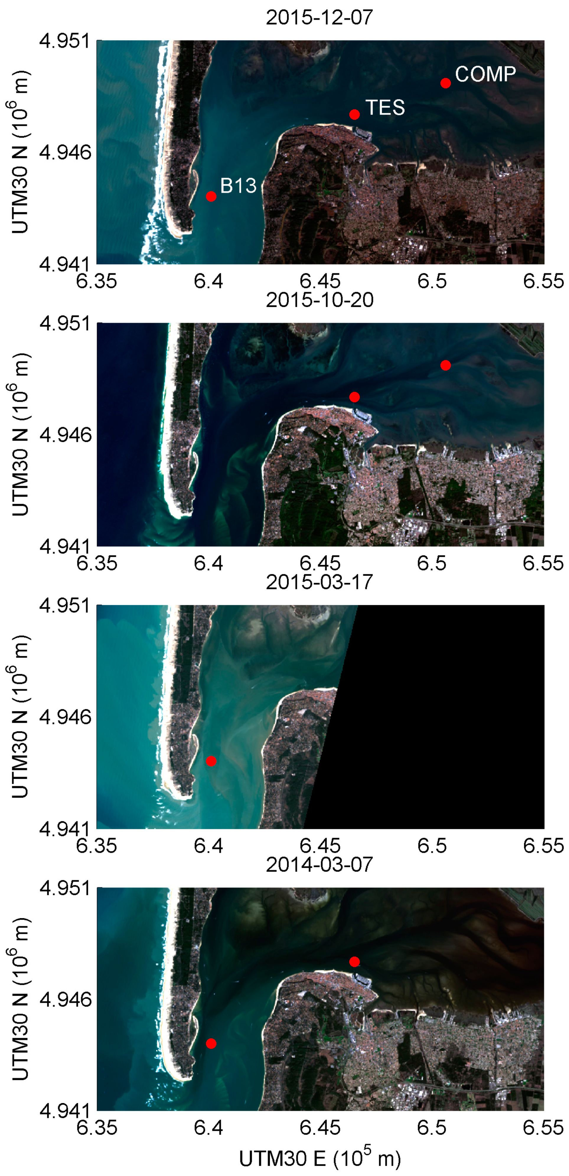
Figure 1. Landsat-8/Operational Land Imager (10-01-2014) image acquired over the Arcachon lagoon area (Southwest France), showing the location of the CIMEL sun photometer (red star) and meteorological (yellow star) stations.
Remotesensing 09 00814 g001
Figure 2. Schematic representation of the in Situ-based Atmospheric CORrection (SACOR) algorithm.
Remotesensing 09 00814 g002
Figure 3. RGB composite (channels 4-3-2) of the four Operational Land Imager (OLI) images associated with ρ w measured in the field (2014-03-07, 2015-03-17, 2015-10-20, and 2015-12-07). For each date, red circles indicate the location of the in-situ measurements used for the composition of the match-up data set. Sampled stations are co-located with the SOMLIT stations (COMP, TES and B13).
Remotesensing 09 00814 g003
Figure 4. Daily mean values of (a) the aerosol optical depth at 500 nm (AOD) and (b) Ångström coefficient computed between 440 and 870 nm ( α 440 870 ) in the period from December 2008–May 2015 at the Aerosol Robotic Network (AERONET) Arcachon lagoon station. Red dotted lines represent the low-pass filtered data performed with running averages.
Remotesensing 09 00814 g004
Figure 5. Mean daily observations of the Ångström coefficient ( α 440 870 ) as a function of the aerosol optical depth at 500 nm (AOD), during December 2008–May 2015 at the AERONET Arcachon lagoon station.
Remotesensing 09 00814 g005
Figure 6. (a) Seasonal volume size distributions and (b) mean monthly fine mode fraction of aerosols in the period from December 2008–May 2015 at the AERONET Arcachon lagoon station. The grey area is associated to the 95% confidence interval.
Remotesensing 09 00814 g006
Figure 7. The whole set of the three-day trajectories ending at the Arcachon lagoon at an altitude level of 1000 m obtained for: (a) class 1; (b) class 2; (c) class 3; (d) class 4; (e) class 5; (f) class 6; and (g) class 7. The centroid of each class is indicated by a red curve and the percentage of air mass back trajectories associated with each class is given in brackets.
Remotesensing 09 00814 g007
Figure 8. Relative frequencies (%) of the trajectory occurrences as a function of the season for the seven classes resulting from the cluster analysis.
Remotesensing 09 00814 g008
Figure 9. Comparison between the SACOR satellite-derived and relative spectral response (RSR)-adjusted in-situ ρ w for the match-up sets (N = 8). Symbols indicate the values of ρ w at the four Operational Land Imager (OLI) spectral bands located in the visible wavelengths. The dashed line represents the 1:1 line.
Remotesensing 09 00814 g009
Figure 10. Comparison between the atmospherically corrected OLI image (bands 1, 2, 3 and 4) and in-situ ρ w (B13 station, see Figure 3) acquired on 2015-10-20. Symbols are associated with the different AC approaches. Note the cross markers are associated with the RSR-adjusted in-situ ρ w values.
Remotesensing 09 00814 g010
Figure 11. Comparison between the SACOR and SWIR-based ACOLITE (ACO-SWIR) atmospherically corrected ρ w at 483, 561 and 655 nm (from top to bottom) from the OLI scene acquired on 2015-10-20. The relative difference between the two products is computed along a 25-km cross-shore transection (red line) starting from the inner part of the lagoon to outer part of the inlet. Vertical dashed lines are associated with sea water optical changes, which are located on the images by black circles.
Remotesensing 09 00814 g011
Table 1. Landsat-8/Operational Land Imager images used in this study, with image identifier, date and time (UTM), and the associated atmospheric conditions (i.e., AOD, α 440 870 and Rh).
ImageDate/Time (UTM)AOD α 440 870 Rh
#1LC08_L1TP_200029_20140307_20170425_01_T12014-03-07 10:490.141.0973%
#2LC08_L1TP_201029_20150317_20170412_01_T12015-03-17 10:540.081.7065%
#3LC08_L1TP_200029_20151020_20170403_01_T12015-10-20 10:480.061.5071%
#4LC08_L1TP_200029_20151207_20170401_01_T12015-12-07 10:480.071.4081%
Table 2. Mean values (standard deviation) of the aerosol optical depth at 500 nm (AOD), the Ångström coefficient ( α 440 870 ) and proportion (%) of the different aerosol types (CM: clean maritime; BU: biomass burning/urban-industrial; DU: desert dust; MM: mixed maritime; and MC: mixed continental) as a function of the season. Note that decimal values for proportions are not significant because the choice of threshold values is partly arbitrary (based on the literature, ±0.02 for AOD and ±0.2 for α 440 870 ). N is the number of observations.
NAODα440–870CMBUDUMMMC
Threshold
Values
---AOD < 0.1
α440–870 < 1.0
AOD > 0.2
α440–870 > 1.0
AOD > 0.2
α440–870 < 1.0
0.1 < AOD < 0.2
α440–870 < 1.0
AOD < 0.2
α440–870 > 1.0
Spring2660.18 (0.11)1.11 (0.36)142281739
Summer2970.14 (0.08)1.20 (0.36)91541161
Fall2130.11 (0.06)1.08 (0.41)23721454
Winter2150.13 (0.10)1.07 (0.47)261311545
Total9910.14 (0.10)1.12 (0.40)171541450
Table 3. Mean values (standard deviation) of the aerosol optical depth at 500 nm (AOD), the Ångström coefficient ( α 440 870 ) and the fine mode fraction (FMF; %) as well as proportion (%) of the different aerosol types (CM: clean maritime; BU: biomass burning/urban-industrial; DU: desert dust; MM: mixed maritime; and MC: mixed continental) for the seven classes resulting from the cluster analysis.
AOD α 440 870 FMFCMBUDUMMMC
Class 10.12 (0.06)0.96 (0.40)56 (19)27722143
Class 20.20 (0.09)1.24 (0.35)65 (18)62671051
Class 30.12 (0.10)1.07 (0.36)56 (19)29821447
Class 40.18 (0.14)1.36 (0.31)74 (17)8282557
Class 50.13 (0.07)1.14 (0.33)61 (15)141081058
Class 60.09 (0.04)0.52 (0.34)36 (16)5200408
Class 70.09 (0.03)0.77 (0.31)48 (16)53003017
Table 4. Relative error (%) between satellite-derived and RSR-adjusted in-situ ρ w (N = 8), which were computed for the four OLI visible bands. The underlined value for each channel is associated with the lowest error.
443 nm483 nm561 nm655 nmMean
SACOR462172224
ACO-SWIR2113271419
ACO-NIR7732362242
6SV-MAR9635173245
6SV-CON7440186549
6SV-TRO8027122436
MACCS7845223846

