LiDAR and Orthophoto Synergy to optimize Object-Based Landscape Change: Analysis of an Active Landslide


Abstract
1. Introduction
2. Materials and Methods
2.1. Data
2.2. Analysis
2.2.1. OBIA: Land Cover
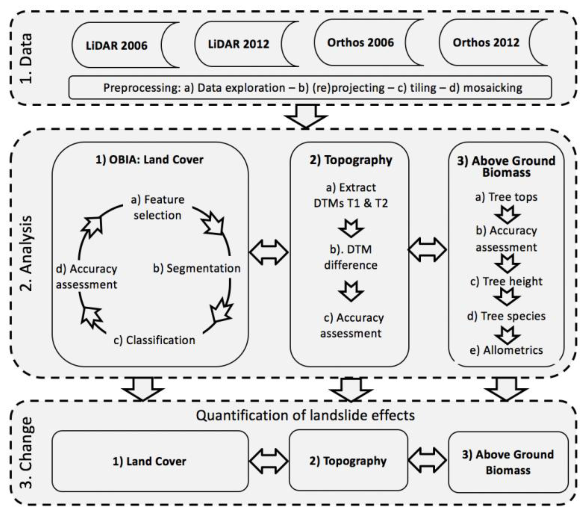
- Feature selection (Figure 2). Land-cover classes have been determined, based on their occurrence in the close surroundings of the landslide affected area, notably: bare soil, grass and shrub land, forest (Norway spruce and beech), water, road and buildings. Feature space optimization (FSO) is used to calculate the feature combinations with the highest separation distance [30]. Two hundred samples per land-cover class were manually classified based on orthophoto recognition. FSO was applied to twelve features derived from either the orthophotos or the LiDAR data. These parameters are: the mean and standard deviation of the red (R), green (G) and blue (B) bands, mean green ratio (G/(R + G + B), mean greenness (1/G), mean brightness, mean CHM, mean length/width ratio and mean rectangular fit.
- Segmentation (Figure 2). To determine the optimal segmentation parameters, an iterative algorithm was developed that produces 125 unique parameter combinations using scale parameter of 10, 20, 30, 40 and 50, shape parameters of 0.1, 0.3, 0.5, 0.7 and 0.9 compactness parameters of 0.1, 0.3, 0.5, 0.7 and 0.9 comparable to the method of Clinton et al. [31]. The resulting objects were then visually compared to the corresponding orthophotos, and evaluated for over-and under segmentation [6]. Additionally, the local-variance based ESP2 tool developed by Drăguţ et al. [32] was used. The smallest scale level determined by the ESP2 tool was 46 for the 2006 and 51 for 2012. Since the methods of Clinton et al. [31] and Drăguţ et al. [32] provided similar results, an average scale parameter of 50 was used. The shape and compactness parameters were selected at 0.3 and 0.5 respectively. Both the spectral information from the orthophotos and the LiDAR-derived canopy height model (CHM) were used as input data for segmentation.
- Classification (Figure 2). The classification consists of two subroutines: (1) a stratified membership classification based on the parameter thresholds obtained through FSO and (2) context-based improvements based on context, geometry, spectral and elevation characteristics. The membership thresholds were deliberately set to be conservative to optimize the workflows’ performance which works well in a diverse heterogeneous landscape such as a landslide. The context-based rulesets improve the classification accuracy after execution of the initial stratified membership-based classification. The context-based rulesets use the spectral characteristics, elevation information and contextual information to tackle shadowing effects, to improve classification of fine-scale features, small open spots in the forest and cope with confusion between bare soil on orthophotos and the LiDAR model. Subsequently, the results of six classifications, three for 2006 and three for 2012, based on a single orthophoto, a single LiDAR dataset and the synergy of both datasets are compared to study the effect on classification accuracy.
- Accuracy assessment (Figure 2). Classification accuracy assessment was performed by random selection of 250–300 objects based on their relative occurrence in the six land-cover classes. A standard confusion error matrix was calculated to include the user and producer accuracies and kappa statistics according to the method described by Congalton [33].
2.2.2. Topography
- DTM difference (Figure 2). The DTM difference was obtained by subtracting DTM 2006 from DTM 2012. Topographical volumetric change was calculated for each land cover class by multiplying the topographical change raster with pixel size (0.125 m × 0125 m).
- Accuracy assessment (Figure 2). To determine the propagation error of DTM differencing the method of Wheaton et al. [34] was used. The propagation error in the DTM differencing process caused maximum uncertainties of 0.29 m. This represents 0.0066 m3 per pixel of volumetric change. Therefore, volumetric changes <0.01 m3 are disregarded and considered as ‘no change areas’, similar to findings of Latypov [35].
2.2.3. Above Ground Biomass
- Accuracy assessment (Figure 2). Assessment of the results generated by the local-maxima algorithm was performed by manual inspection and comparison of the generated canopy tops with the CHM and orthophotos in a 3D ArcScene environment, which allows for detailed zooming and panning.
- Tree height (Figure 2). Individual tree height was calculated by multiplying the rasterized CHM with the binary tree top locations.
- Allometrics (Figure 2). According to Maier et al. [12] and the Austrian Forest Inventory [37] the Norway Spruce and Beech are the dominant tree species in Vorarlberg. Therefore, the allometric equations for AGB calculation for Norway Spruce and Austrian Beech were used [38,39,40]:Norway Spruce DBH = e((0.1687+1.2413*ln(H)),where DBH = diameter at breast height (cm) and H = tree height (m)Beech DBH = (H/3.240838)1/0.613065,Norway Spruce B = e(-4.63873+(2.75352*ln((DBH)-0.08578*ln(H))),where B = biomass (kg)Beech B = −2.872 + 2.095 * ln(DBH) + 0.678 * ln(H),
2.3. Change Analysis: Land Cover, Topography and Above Ground Biomass
3. Results
3.1. Land-Cover Change
3.2. Topographical Change
3.3. Above-Ground Biomass Change
4. Discussion
5. Conclusions
Acknowledgments
Author Contributions
Conflicts of Interest
References
- Eitel, J.U.; Höfle, B.; Vierling, L.A.; Abellán, A.; Asner, G.P.; Deems, J.S.; Glennie, C.L.; Joerg, P.C.; LeWinter, A.L.; Magney, T.S. Beyond 3-d: The new spectrum of LiDAR applications for earth and ecological sciences. Remote Sens. Environ. 2016, 186, 372–392. [Google Scholar] [CrossRef]
- Jaboyedoff, M.; Oppikofer, T.; Abellán, A.; Derron, M.-H.; Loye, A.; Metzger, R.; Pedrazzini, A. Use of LiDAR in landslide investigations: A review. Nat. Hazards 2012, 61, 5–28. [Google Scholar] [CrossRef]
- Machala, M.; Zejdová, L. Forest mapping through object-based image analysis of multispectral and LiDAR aerial data. Eur. J. Remote Sens. 2014, 47, 117–131. [Google Scholar] [CrossRef]
- Wulder, M.A.; Seemann, D. Forest inventory height update through the integration of LiDAR data with segmented landsat imagery. Can. J. Remote Sens. 2003, 29, 536–543. [Google Scholar] [CrossRef]
- Zhou, W.; Troy, A.; Grove, M. Object-based land cover classification and change analysis in the Baltimore metropolitan area using multi-temporal high resolution remote sensing data. Sensors 2008, 8, 1613–1636. [Google Scholar] [CrossRef] [PubMed]
- Martha, T.R.; Kerle, N.; van Westen, C.J.; Jetten, V.; Kumar, K.V. Object-oriented analysis of multi-temporal panchromatic images for creation of historical landslide inventories. ISPRS J. Photogramm. Remote Sens. 2012, 67, 105–119. [Google Scholar] [CrossRef]
- Van Den Eeckhout, M.; Kerle, N.; Poesen, J.; Hervás, J. Object-oriented identification of forested landslides with derivatives of single pulse LiDAR data. Geomorphology 2012, 173, 30–42. [Google Scholar] [CrossRef]
- Lahousse, T.; Chang, K.; Lin, Y. Landslide mapping with multi-scale object-based image analysis—A case study in the Baichi watershed, Taiwan. Nat. Hazard Earth Sys. 2011, 11, 2715–2726. [Google Scholar] [CrossRef]
- Li, X.; Cheng, X.; Chen, W.; Chen, G.; Liu, S. Identification of forested landslides using LiDAR data, object-based image analysis, and machine learning algorithms. Remote Sens. 2015, 7, 9705–9726. [Google Scholar] [CrossRef]
- Rutzinger, M.; Zieher, T.; Pfeiffer, J.; Schlögel, R.; Darvishi, M.; Toschi, I.; Remondino, F. In Evaluating Synergy Effects of Combined Close-Range and Remote Sensing Techniques for the Monitoring of a Deep-Seated Landslide (Schmirn, Austria). EGU General Assembly Conference Abstracts. 2017, p. 6393. Available online: http://adsabs.harvard.edu/abs/2017EGUGA.19.6393R (accessed on 26 July 2017).
- Frodella, W.; Ciampalini, A.; Gigli, G.; Lombardi, L.; Raspini, F.; Nocentini, M.; Scardigli, C.; Casagli, N. Synergic use of satellite and ground-based remote sensing methods for monitoring the San Leo rock cliff (northern Italy). Geomorphology 2016, 264, 80–94. [Google Scholar] [CrossRef]
- Aguirre-Gutiérrez, J.; Seijmonsbergen, A.C.; Duivenvoorden, J.F. Optimizing land cover classification accuracy for change detection, a combined pixel-based and object-based approach in a mountainous area in Mexico. Appl. Geogr. 2012, 34, 29–37. [Google Scholar] [CrossRef]
- Wang, L.; Sousa, W.; Gong, P. Integration of object-based and pixel-based classification for mapping mangroves with Ikonos imagery. Int. J. Remote Sens. 2004, 25, 5655–5668. [Google Scholar] [CrossRef]
- Blaschke, T. Object based image analysis for remote sensing. ISPRS J. Photogramm. Remote Sens. 2010, 65, 2–16. [Google Scholar] [CrossRef]
- Chen, Y.; Su, W.; Li, J.; Sun, Z. Hierarchical object oriented classification using very high resolution imagery and LiDAR data over urban areas. Adv. Space Res.-Ser. 2009, 43, 1101–1110. [Google Scholar] [CrossRef]
- Ke, Y.; Quackenbush, L.J.; Im, J. Synergistic use of Quickbird multispectral imagery and LiDAR data for object-based forest species classification. Remote Sens. Environ. 2010, 114, 1141–1154. [Google Scholar] [CrossRef]
- Maier, B.; Tiede, D.; Dorren, L. Assessing mountain forest structure using airborne laser scanning and landscape metrics. Int. Arch. Photogramm. Remote Sens. Spat. Inf. Sci. 2006, 36, C42. [Google Scholar]
- Chen, L.; Chiang, T.; Teo, T. In Fusion of LiDAR data and high resolution images for forest canopy modelling. In Proceedings of the 26th Asian Conference on Remote Sensing, Hanoi, Vietnam, 7–11 November 2005; Available online: https://www.researchgate.net/profile/Tee_Ann_Teo/publication/228850651_Fusion_of_LIDAR_data_and_high_resolution_images_for_forest_canopy_modeling/links/564ec4fd08aeafc2aab1e664.pdf (accessed on 26 July 2017).
- Hermosilla, T.; Almonacid, J.; Fernández-Sarría, A.; Ruiz, L.; Recio, J. Combining features extracted from imagery and LiDAR data for object-oriented classification of forest areas. Int. Arch. Photogramm. Remote Sens. Spat. Inf. Sci. 2010, 38, 194–200. Available online: http://www.isprs.org/proceedings/xxxviii/4-c7/pdf/hermosilla_148.pdf (accessed on 26 July 2017).
- Hudak, A.T.; Evans, J.S.; Stuart Smith, A.M. LiDAR utility for natural resource managers. Remote Sens. 2009, 1, 934–951. [Google Scholar] [CrossRef]
- Mücher, C.A.; Roupioz, L.; Kramer, H.; Bogers, M.; Jongman, R.H.; Lucas, R.M.; Kosmidou, V.; Petrou, Z.; Manakos, I.; Padoa-Schioppa, E. Synergy of airborne LiDAR and Worldview-2 satellite imagery for land cover and habitat mapping: A bio-sos-eodham case study for the Netherlands. Int. J. Appl. Earth Obs. 2015, 37, 48–55. [Google Scholar] [CrossRef]
- Syed, S.; Dare, P.; Jones, S. Automatic Classification of Land Cover Features with High Resolution Imagery and LiDAR Data: An Object-Oriented Approach. Available online: https://pdfs.semanticscholar.org/47a3/6f82098005121b419e6b24ee6de18bb90702.pdf (accessed on 26 July 2017).
- Parent, J.R.; Volin, J.C.; Civco, D.L. A fully-automated approach to land cover mapping with airborne LiDAR and high resolution multispectral imagery in a forested suburban landscape. ISPRS J. Photogramm. Remote Sens. 2015, 104, 18–29. [Google Scholar] [CrossRef]
- Debes, C.; Merentitis, A.; Heremans, R.; Hahn, J.; Frangiadakis, N.; van Kasteren, T.; Liao, W.; Bellens, R.; Pižurica, A.; Gautama, S. Hyperspectral and LiDAR data fusion: Outcome of the 2013 GRSS data fusion contest. IEEE J. Sel. Top. Appl. 2014, 7, 2405–2418. [Google Scholar] [CrossRef]
- Khosravipour, A.; Skidmore, A. K.; Wang, T.; Isenburg, M.; Khoshelham, K. Effect of slope on treetop detection using a LiDAR canopy height model. ISPRS J. Photogramm. Remote Sens. 2015, 104, 44–52. [Google Scholar] [CrossRef]
- Ghuffar, S.; Székely, B.; Roncat, A.; Pfeifer, N. Landslide displacement monitoring using 3D range flow on airborne and terrestrial LiDAR Data. Remote Sens. 2013, 5, 2720–2745. [Google Scholar] [CrossRef]
- Roncat, A.; Ghuffar, S.; Székely, B.; Dorninger, P.; Rasztovits, S.; Mittelberger, M.; Koma, Z.; Krawczyk, D.; Pfeifer, N. A natural laboratory—Terrestrial laser scanning and auxiliary measurements for studying an active landslide. In Proceedings of the 2nd Joint International Symposium on Deformation Monitoring (JISDM), Nottingham, United Kingdom, 9–10 September 2013; Available online: https://www.researchgate.net/publication/258029296_A_Natural_LaboratoryTerrestrial_Laser_Scanning_and_auxiliary_Measurements_for_studying_an_active_Landslide (accessed on 26 July 2017).
- Sithole, G.; Vosselman, G. Experimental comparison of filter algorithms for bare-earth extraction from airborne laser scanning point clouds. ISPRS J. Photogramm. Remote Sens. 2004, 59, 85–101. [Google Scholar] [CrossRef]
- Geoland.at ist das Geoportal der österreichischen Länder. Es ermöglicht den einfachen Zugriff auf raumbezogene Informationen. Available online: http://www.vorarlberg.at/vorarlberg/bauen_wohnen/bauen/vermessung_geoinformation/weitereinformationen/services/geoland_at.htm (accessed on 26 September 2016).
- Platt, R.V.; Rapoza, L. An evaluation of an object-oriented paradigm for land use/land cover classification. Prof. Geogr. 2008, 60, 87–100. [Google Scholar] [CrossRef]
- Clinton, N.; Holt, A.; Scarborough, J.; Yan, L.; Gong, P. Accuracy assessment measures for object-based image segmentation goodness. Photogramm. Eng. Remote Sens. 2010, 76, 289–299. [Google Scholar] [CrossRef]
- Drăguţ, L.; Csillik, O.; Eisank, C.; Tiede, D. Automated parameterisation for multi-scale image segmentation on multiple layers. ISPRS J. Photogramm. Remote Sens. 2014, 88, 119–127. [Google Scholar] [CrossRef] [PubMed]
- Congalton, R.G. A review of assessing the accuracy of classifications of remotely sensed data. Remote Sens. Environ. 1991, 37, 35–46. [Google Scholar] [CrossRef]
- Wheaton, J.M.; Brasington, J.; Darby, S.E.; Sear, D.A. Accounting for uncertainty in DEMs from repeat topographic surveys: Improved sediment budgets. Earth Surf. Processes. Landf. 2010, 35, 136–156. [Google Scholar] [CrossRef]
- Latypov, D. Estimating relative LiDAR accuracy information from overlapping flight lines. ISPRS J. Photogramm. Remote Sens. 2002, 56, 236–245. [Google Scholar] [CrossRef]
- Martin, K.; Schroeder, W.; Lorensen, W. Definiens Developer XD 2.0.4. Reference Book, 2nd ed.; Definiens AG: Munich, Germany, 2012; pp. 1–414. [Google Scholar]
- Austrian Forest Report 2015—BMLFUW. Available online: https://www.bmlfuw.gv.at/dam/jcr...8259.../Austrian%20Forest%20Report%202015.pdf (accessed on 17 February 2017).
- Muukonen, P.; Heiskanen, J. Estimating biomass for boreal forests using ASTER satellite data combined with standwise forest inventory data. Remote Sens. Environ. 2005, 99, 434–447. [Google Scholar] [CrossRef]
- Zianis, D.; Muukkonen, P.; Mäkipää, R.; Mencuccini, M. Biomass and Stem Volume Equations for Tree Species in Europe. Available online: http://urn.fi/URN:ISBN:951-40-1984-9 (accessed on 26 July 2017).
- Widlowski, J.; Verstraete, M.; Pinty, B.; Gobron, N. Allometric Relationships of Selected European Tree Species. Report EUR 20855 EN. 2003. Available online: http://publications.jrc.ec.Europa.eu/repository/bitstream/JRC26286/EUR%2020855%20EN.pdf (accessed on 26 July 2017).
- Arroyo, L.A.; Johansen, K.; Armston, J.; Phinn, S. Integration of LiDAR and Quickbird imagery for mapping riparian biophysical parameters and land cover types in Australian tropical savannas. For. Ecol. Manag. 2010, 259, 598–606. [Google Scholar] [CrossRef]
- Kakunda, C. Synergy of Airborne LiDAR Data and VHR Satellite Optical Imagery for Individual Crown and Tree Species Identification. Master’s Thesis, University of Twente, Enschede, The Netherlands, 2013. Available online: http://www.itc.nl/library/papers_2013/msc/gem/kukunda.Pdf (accessed on 26 July 2017).
- Liu, X. Airborne LiDAR for DEM generation: Some critical issues. Prog. Phys. Geogr. 2008, 32, 31–49. [Google Scholar] [CrossRef]
- Aguilar, F.J.; Mills, J.P.; Delgado, J.; Aguilar, M.A.; Negreiros, J.; Pérez, J.L. Modelling vertical error in LiDAR-derived digital elevation models. ISPRS J. Photogramm. Remote Sens. 2010, 65, 103–110. [Google Scholar] [CrossRef]
- Vazirabad, Y.F.; Karslioglu, M.O. LiDAR for Biomass Estimation. Available online: http://cdn.intechopen.com/pdfs/19065/InTech-LiDAR_for_biomass_estimation.pdf (accessed on 26 July 2017).
- Brasington, J.; Langham, J.; Rumsby, B. Methodological sensitivity of morphometric estimates of coarse fluvial sediment transport. Geomorphology 2003, 53, 299–316. [Google Scholar] [CrossRef]
- Wulder, M.A.; Bater, C.W.; Coops, N.C.; Hilker, T.; White, J.C. The role of LiDAR in sustainable forest management. For. Chron. 2008, 84, 807–826. [Google Scholar] [CrossRef]
- Sailer, R.; Rutzinger, M.; Rieg, L.; Wichmann, V. Digital elevation models derived from airborne laser scanning point clouds: Appropriate spatial resolutions for multi-temporal characterization and quantification of geomorphological processes. Earth Surf. Process. Landf. 2014, 39, 272–284. [Google Scholar] [CrossRef]
- Su, J.; Bork, E. Influence of vegetation, slope, and LiDAR sampling angle on DEM accuracy. Photogramm. Eng. Remote Sens. 2006, 72, 1265–1274. [Google Scholar] [CrossRef]
- Anders, N.; Seijmonsbergen, A.C.; Bouten, W. Geomorphological change detection using object-based feature extraction from multi-temporal LiDAR data. IEEE Geosci. Remote Sens. Lett. 2013, 10, 1587–1591. [Google Scholar] [CrossRef]
- Jochem, A.; Hollaus, M.; Rutzinger, M.; Höfle, B.; Schadauer, K.; Maier, B. Estimation of aboveground biomass using airborne LiDAR Data. In Proceedings of the 10th International Conference on LiDAR Applications for Assessing Forest Ecosystems, Freiburg, Germany, 14–17 September 2010; Available online: https://pdfs.semanticscholar.org/a230/236f44b3770ba6ab579f509cad551b75b106.pdf (accessed on 26 July 2017).
- Popescu, S.C. Estimating biomass of individual pine trees using airborne LiDAR. Biomass Bioenergy 2007, 31, 646–655. [Google Scholar] [CrossRef]
- Pouliot, D.; King, D.; Bell, F.; Pitt, D. Automated tree crown detection and delineation in high-resolution digital camera imagery of coniferous forest regeneration. Remote Sens. Environ. 2002, 82, 322–334. [Google Scholar] [CrossRef]
- Hollaus, M.; Dorigo, W.; Wagner, W.; Schadauer, K.; Höfle, B.; Maier, B. Operational wide-area stem volume estimation based on airborne laser scanning and national forest inventory data. Int. J. Remote Sens. 2009, 30, 5159–5175. [Google Scholar] [CrossRef]
- Lefsky, M.A.; Harding, D.; Cohen, W.; Parker, G.; Shugart, H. Surface LiDAR remote sensing of basal area and biomass in deciduous forests of eastern Maryland, USA. Remote Sens. Environ. 1999, 67, 83–98. [Google Scholar] [CrossRef]
- Bräuer, T.; Tuttas, S. Analyse und Management von Regionaltypischen Naturgefahren am Beispiel Einer Hangrutschung in Doren (Vorarlberg); 2010; pp. 389–402. Available online: http://web23.shm.wissner.com/sites/default/files/landesverband/bayern/anhang/beitragskontext/2014/braeuer_3_2010.pdf (accessed on 26 July 2017).
- Casagli, N.; Frodella, W.; Morelli, S.; Tofani, V.; Ciampalini, A.; Intrieri, E.; Lu, P. Spaceborne, UAV and ground-based remote sensing techniques for landslide mapping, monitoring and early warning. Geoenviron. Disasters 2017, 4, 1–23. [Google Scholar] [CrossRef]
- Blaschke, T.; Burnett, C.; Pekkarinen, A. Image segmentation methods for object-based analysis and classification. In Remote Sensing Image Analysis: Including the Spatial Domain; Jong, S.M.D., Meer, F.D.V., Eds.; Springer: Dordrecht, The Netherlands, 2004; Volume 5, pp. 211–236. ISBN 978-1-4020-2560-0. [Google Scholar]
- Desclée, B.; Bogaert, P.; Defourny, P. Forest change detection by statistical object-based method. Remote Sens. Environ. 2006, 102, 1–11. [Google Scholar] [CrossRef]


| Year | Data Type | Extension | Camera | Accuracy |
|---|---|---|---|---|
| 2006 | TCO | .img | Zeiss RMK TOP 30/23 | Resolution: 0.125 m × 0.125 m |
| LiDAR | .img | ALTM 2050 | Point density: 2/m2 | |
| Height accuracy: 0.1 m | ||||
| Location accuracy: 0.2 m | ||||
| Vertical accuracy: <0.25 m | ||||
| Horizontal accuracy: <0.3 m | ||||
| 2012 | TCO | .img | Vexcel Ultracam XP | Resolution: 0.125 m × 0.125 m |
| LiDAR | .laz | Harrier 56-009 | Point density: 4–8 m2 | |
| Height accuracy: 0.075 m | ||||
| Location accuracy: 0.1 m | ||||
| Vertical accuracy: <0.15 m | ||||
| Horizontal accuracy: 0.25 m |
| VHR Orthophoto | LiDAR | Data Synergy | ||
|---|---|---|---|---|
| 2006 | OA | 0.76 | 0.65 | 0.90 |
| KS | 0.64 | 0.46 | 0.83 | |
| 2012 | OA | 0.75 | 0.64 | 0.91 |
| KS | 0.61 | 0.48 | 0.93 |
| Confusion Matrix | Bare Soil | Building | Grassland | Road | Trees | Water | Sum |
|---|---|---|---|---|---|---|---|
| Bare soil | 36 | 0 | 1 | 1 | 1 | 0 | 39 |
| Building | 0 | 5 | 0 | 0 | 0 | 0 | 5 |
| Grassland | 2 | 0 | 63 | 1 | 6 | 0 | 72 |
| Road | 2 | 0 | 1 | 12 | 0 | 0 | 15 |
| Trees | 1 | 0 | 4 | 1 | 117 | 0 | 123 |
| Water | 2 | 0 | 0 | 0 | 0 | 11 | 13 |
| Sum | 43 | 5 | 69 | 15 | 124 | 11 | 267 |
| Producer | 0.84 | 1.00 | 0.91 | 0.80 | 0.94 | 1.00 | |
| User | 0.92 | 1.00 | 0.88 | 0.80 | 0.95 | 0.85 | |
| Overall accuracy: 0.91 Kappa statistic: 0.93 Contextual improvements: +0.18 | |||||||
| Year | Bare Soil | Building | Grass | Road | Trees | Water | Total | |
|---|---|---|---|---|---|---|---|---|
| 2006 | Sum (m2) | 52,484.3 | 680.2 | 86,111.4 | N.A. | 241,721.6 | 1552.3 | 382,550 |
| Percent (%) | 13.7 | 0.2 | 22.5 | N.A. | 63.2 | 0.4 | ||
| 2012 | Sum (m2) | 41,458.0 | 532.7 | 92,694.4 | 2364.2 | 244,386.0 | 1114.6 | |
| Percent (%) | 10.8 | 0.1 | 24.2 | 0.6 | 63.9 | 0.3 | ||
| 2006–2012 | Change (%) | −2.9 | −0.1 | +1.7 | +0.6 | +0.7 | −0.1 |
| GtG | GtB | GtT | GtR | BtB | BtG | |
|---|---|---|---|---|---|---|
| Sum (m2) | 51,405.0 | 10,274.1 | 23,078.7 | 1287.3 | 24,773.1 | 22,204.8 |
| Change (%) | 13.4 | 2.7 | 6.0 | 0.3 | 6.5 | 5.8 |
| BtT | BtR | TtT | TtG | TtB | TtR | |
| Sum (m2) | 4612.2 | 337.8 | 215,888.2 | 19,082.7 | 6096.93 | 653.2 |
| Change (%) | 1.2 | 0.1 | 56.4 | 5.0 | 1.6 | 0.2 |
| Number (#) | Biomass (kg) | |
|---|---|---|
| 2006 | 1451 | 751,771 |
| 2012 | 1458 | 654,789 |
| Change | +7 | −62,134 |
© 2017 by the authors. Licensee MDPI, Basel, Switzerland. This article is an open access article distributed under the terms and conditions of the Creative Commons Attribution (CC BY) license (http://creativecommons.org/licenses/by/4.0/).
Share and Cite
Kamps, M.; Bouten, W.; Seijmonsbergen, A.C. LiDAR and Orthophoto Synergy to optimize Object-Based Landscape Change: Analysis of an Active Landslide. Remote Sens. 2017, 9, 805. https://doi.org/10.3390/rs9080805
Kamps M, Bouten W, Seijmonsbergen AC. LiDAR and Orthophoto Synergy to optimize Object-Based Landscape Change: Analysis of an Active Landslide. Remote Sensing. 2017; 9(8):805. https://doi.org/10.3390/rs9080805
Chicago/Turabian StyleKamps, Martijn, Willem Bouten, and Arie, C. Seijmonsbergen. 2017. "LiDAR and Orthophoto Synergy to optimize Object-Based Landscape Change: Analysis of an Active Landslide" Remote Sensing 9, no. 8: 805. https://doi.org/10.3390/rs9080805
APA StyleKamps, M., Bouten, W., & Seijmonsbergen, A. C. (2017). LiDAR and Orthophoto Synergy to optimize Object-Based Landscape Change: Analysis of an Active Landslide. Remote Sensing, 9(8), 805. https://doi.org/10.3390/rs9080805