Article

Modelling Shadow Using 3D Tree Models in High Spatial and Temporal Resolution

Chair of Forest Growth and Dendroecology, Albert-Ludwigs-University Freiburg, Tennenbacher Street 4, 79106 Freiburg, Germany
*
Author to whom correspondence should be addressed.
Remote Sens. 2017, 9(7), 719; https://doi.org/10.3390/rs9070719
Submission received: 24 May 2017 / Revised: 29 June 2017 / Accepted: 9 July 2017 / Published: 13 July 2017

Abstract

:
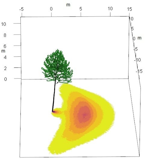
Information about the availability of solar irradiance for crops is of high importance for improving management practices of agricultural ecosystems such as agroforestry systems (AFS). Hence, the development of a high-resolution model that allows for the quantification of tree shading on a diurnal and annual time scale is highly demanded to generate realistic estimations of the shading dynamics in a given AFS. We describe an approach using 3D data derived from a terrestrial laser scanner and the steps undertaken to develop a vector-based model that quantifies and visualizes the shadow cast by single trees at daily, monthly, seasonal or annual levels with the input of cylinder-based tree models. It is able to compute the shadow of given tree models in time intervals of 10 min. To simulate seasonal growth and shedding of leaves, ellipsoids as replacement for leaves can be added to the tips of the tree model’s branches. The shadow model is flexible in its input of location (latitude, longitude), tree architecture and temporal resolution. Due to the possibility to feed this model with factual climate data such as cloud covers, it represents the first 3D tree model that enables the user to retrospectively analyze the shadow regime below a given tree, and to quantify shadow-related developments in AFS.

Graphical Abstract

1. Introduction

Plant growth depends on light interception. Hence, information about the availability of solar irradiance is of high importance for understanding and improving management practices of natural and agricultural ecosystems. Regarding the latter, estimations of solar irradiation availability are of particular interest for managing agroforestry systems (AFS). In these systems, woody perennials such as trees are deliberately grown together with agricultural crops and/or animals on the same land unit, resulting in a significant interaction of the AFS components with regard to the utilization of water, nutrients and light [1]. On the one hand, a significant reduction of the light interception for the agricultural crops growing below trees can result in a drastic reduction of the crop productivity in case of light-demanding C4-species [2], and on the other hand, more shade tolerant crop species may even react positively to shading, as demonstrated by tobacco (Nicotiana tabacum L.) [3], Coffea arabica L. [4] or American ginseng (Panax quinquefolium L.) [5]. To generate realistic estimations of the shadows cast in a given AFS, the development of a model that allows for the detailed quantification of tree shading on a diurnal and annual time scale is highly demanded.
One approach to model tree shadow and the resulting light availability on the ground below relies on constructing a virtual ellipsoid that covers the crown of a three-dimensional tree model [6]. To advance this model, the application of this technique, in combination with the refinement of the output results, was improved by using a leaf-clumping index [7]. However, the authors came to the conclusion that modelling and predicting detailed light availability distributions under an individual tree cannot be accomplished by models which use the ellipsoid as a representation of a whole tree crown. These ellipsoids are not able to approximate realistic crown shapes of individual trees, as tree crowns can be very variable, thus featuring considerable morphological differences that influence the leaf area distribution (LAD) and, therefore, the radiation regime below them [7,8]. Other results showed that more details on the tree crown structure are necessary in order to generate detailed predictions of light availability under a tree [9,10]. The heterogeneous tree crowns induce heterogeneous light conditions for the crops under the tree including the sun fleck regime, which is highly variable in time and space [11]. A complicated consecutive process in using either the ellipsoid [7,12] or voxel approach [13,14,15,16] is the measurement and usage of the leaf area index (LAI) and/or the LAD with uniform or random hypotheses for LAD. However, both hypotheses lead to an underestimation of shading [7]. Several authors tried to increase the accuracy of voxel-based LAD modelling but faced difficulties when correcting for vegetation clumping, occlusion effects and the presence of woody structures [16,17]. A promising technique when using the voxel-based approach is shown in [15], where the LAD could be directly derived by transforming the TLS data into small leaf-sized voxels.
As of today, light models that utilize and generate detailed shading information from individual trees based on a high resolution 3D model of single trees are not available. In the following sections, we present the initial steps of the development of a model that enables predictions of shadow and light distributions below individual single trees in the course of the year with flexible temporal resolutions. Our data are derived from the utilization of terrestrial laser scanning (TLS). At present, TLS provides the most accurate measurements of complex 3D structures such as trees. Based on the TLS point cloud obtained from a single tree, a light model was created that allows for computing the shadow of this tree onto the ground below with regard to its intensity and changes throughout the year. This model can be fed with TLS point clouds converted to cylinder models gained from any other tree, and can thus be utilized to quantify the shading effect of any tree of interest. Utilizing such models, the management of AFS, but also the management of other ecosystems in which a precise quantification of solar irradiance is of importance, can be optimized.

2. Materials and Methods

2.1. The Scanned Tree and Its Location

To develop the light model in question, we scanned a cherry tree (Prunus avium L.) growing on an experimental AFS site in SW-Germany close to Breisach (48°4′24″N; 7°35′26″E, 182 m a.s.l.) with a terrestrial laser scanner (TLS). As the cherry tree is a deciduous, broad-leaved tree, we scanned the tree in winter to be able to generate a 3D tree model that comprises all branches without being occluded by leaves. The scans were performed with the phase shift scanner Z+F IMAGER 5010 (Zoller+Fröhlich GmbH, Wangen, Germany). Detailed information about the scanning can be found in a previous publication [18]. At the time of scanning, the cherry tree was 19 years old, 11.02 m high and had a diameter at breast height of 16.8 cm. The climate at the experimental site is temperate and mild with a mean annual air temperature of 11.2 °C and a mean annual precipitation sum of 710 m for the growing period of the tree (1997–2012). A detailed description of the site, soils and climate conditions can be found in [19].

2.2. Input Data

To develop our new model, the TLS data of the relevant tree are first used as input for the open source Software SimpleTree [20], which computes highly accurate cylinder models of trees from point clouds. Subsequently, this 3D cylinder model serves as basis for the following steps. To calculate the dimensions of the casted shadow, the exact position of the sun during the days of a calendar year needs to be taken into account. Hence, the unit vector in the direction of the sun from the position of the observer, in our case the position of the tree, is calculated using the package insol in R [21]. With this R package, the unit vector and the sun position in Cartesian coordinates are calculated and used to determine the azimuth and zenith angles of the sun. Additional output results comprise information on each Julian day, such as its date as well as the times of the day. These data are required for the further development steps.
For our purpose, the output of the insol calculations is used for 10-min time intervals. Solar irradiance data were obtained from the German Meteorological Service (Deutscher Wetterdienst, DWD) which provides them in hourly sums of global short wave and diffuse irradiance in J cm−2 [22]. We used the insolation data provided by the nearest meteorological station in Freiburg, which is located about 20 km east of the study site. The data values were converted into kWh m−2 for further processing. To gain general information on the shadow and to avoid a weather-related bias, we calculated the long-term monthly means of global and diffuse irradiance in hourly sums from 1977 to 2015, assuming a cloudless sky. The methods used to gain information on the dimension of the shadow and its changes during the year are described below. All following steps are implemented in the open source language R, version 3.3.2 [23].

2.3. Pre-Calculations

To model sun beams striking the tree, the available Cartesian coordinates of the sun’s position are transformed into spherical coordinates by means of the astronomical unit rounded up to 150 × 106 km. To reduce the processing time, the sun beams are only calculated when the sun is in the diurnal arc, that is, if the zenith is lower than 90 degrees. Other sun positions, such as the sun being below the horizon, are not considered. Moreover, we treat all sun beams hitting the tree as running in parallel in our model, given the large distance of the sun and the comparably small size of our tree. Consequently, due to this parallel projection approach, all sun beams strike the tree in the same insolation angle in our calculations.

2.4. Computing Vertices of Cylinders as a Base for Tree Shadow Projections

The shadow calculations developed in the present study predicate on the already mentioned software SimpleTree. This software generates tree models that consist of cylinders of different sizes and angles of their axes. Each cylinder is comprised of two identical circles—the base areas—and a shell surface. For our calculations of the shadow of trees, we first extract the cylinders’ base centers as Cartesian coordinates and the cylinders’ radiuses from SimpleTree. However, to generate realistic shadow projections, more than one projection point per cylinder top and bottom are required. Due to the sun’s movement along the ecliptic and the angle of the modeled cylinders in relation to the earth’s surface, the projected shadows of the cylinders’ top and bottom typically assume the shapes of ellipses. Each ellipse has a semi-minor axis and a semi-major axis, which are orthogonal to each other and end in the ellipse’s vertices. To generate an elliptic shadow of a circle, the four vertices of both semi axes and their orientation towards the sun need to be determined. In our case, their positions are calculated by means of the cross product according to the following procedure:
The points A (top) and B (bottom) are the cylinder base centers (Figure 1a). Points C and D on the top base must lie on a straight line, on one of the semi axes. Points that lie on one of the semi axes on the top base area must fulfill two conditions. First, the line must be arranged orthogonally to the cylinder rotation axis through the base centers A and B. This ensures that the points lie on the plane of the base, not below or above it. Thereby, it is warranted that the potential inclination of the cylinder is integrated in the calculations. Additionally, the line must be arranged orthogonally to the sun ray vector. This condition guarantees that the points of contact between the sun’s directional tangent and the cylinder base can be found. This vector ( a c ) can be calculated with the cross product (1), which is a binary operation on the two vectors ( a b and s a ), where both vectors are perpendicular to the cross product a c (Figure 1b).
a b × s a = a c ,
The cross product results in two unit vectors in opposite directions running left and right of the base center. When the linear Equation (2) is solved in a parameter form where A is the position vector, the unit vectors show in both directions, and r represents the radius of the base, the first two intercept points on the base needed for shadow projection can be determined.
The next straight is calculated as the cross product (3) between vector a c and the rotation axis vector a b (Figure 1). Subsequently, the Equation (4) is solved with picking radius r as length of the straight. The points of intersection of the sun rays with the cylinder bottom are derived with the same procedure.
A + r ×   ±   a c   =   C , D ,
a b × a c = a e ,
A + r ×   ±   a e   =   E , F ,

2.5. Projecting the Cylinder Shadow onto the Ground and Calculating Energy Loss Due to Shading

Following the procedure described above, the four vertices of the cylinder top and the four vertices of the cylinder bottom in relation to a given position of the sun can be computed and the shadow of the cylinder can be projected to the ground. This is performed using a parallel projection. Subsequently, the ellipses’ vertices are connected with a convex hull to link the cylinder base projections as a polygon shape. This envelope defines the shadow of one cylinder, and is converted into the format of a spatial data polygon. To quantify the loss of energy on the ground through shading, the polygons of the tree shadow on the x-y-plane are aggregated with a raster consisting of cells with a resolution of 10 cm × 10 cm. Each raster cell contains a binary value of existing (YES) or non-existing shadow (NO). The binary value is further transformed into the values for diffuse (YES) or global (NO) irradiance, due to the attribute of diffuse radiation to create no shadow. Each raster cell is assigned with the information about solar irradiance in 10-min intervals. The hourly sums of the DWD are adapted to this frequency and are accumulated further to monthly energy sums (kWh m−2) of each cell in the grid. The monthly sums are smoothed with a simple general additive model to account for the 10-min intervals. As a first validation, the maximum possible energy gained in one grid cell without any shading effect matches the monthly sum derived directly from the measured data.

2.6. Computing Ellipsoids to Simulate Leaves

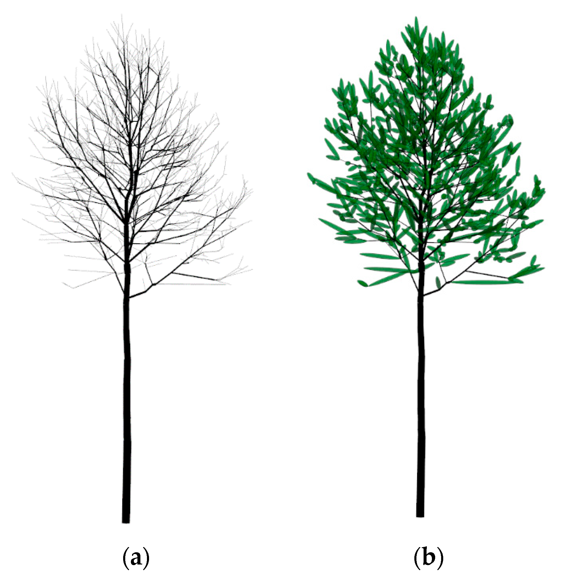
To gain a more realistic view on the shadow cast by a tree throughout the year, we divided the appearance of the tree in a “leaf-on”-type, representing its state during the vegetation period, and a “leaf-off”-type for the rest of the year. Since the tree used for modeling was scanned in the leafless state in October 2013, we use the leafless tree model of the scan for the period of October 2013 until March 2014. For the period of April 2014 until September 2014, we use a theoretical approach to add calculated leaf-like shapes around the twigs of the tree model, assuming that each cylinder with a radius smaller than 0.5 cm grows leaves. Hence, we adjoined computed ellipsoids around these twigs, mimicking a set of leaves (Figure 2).
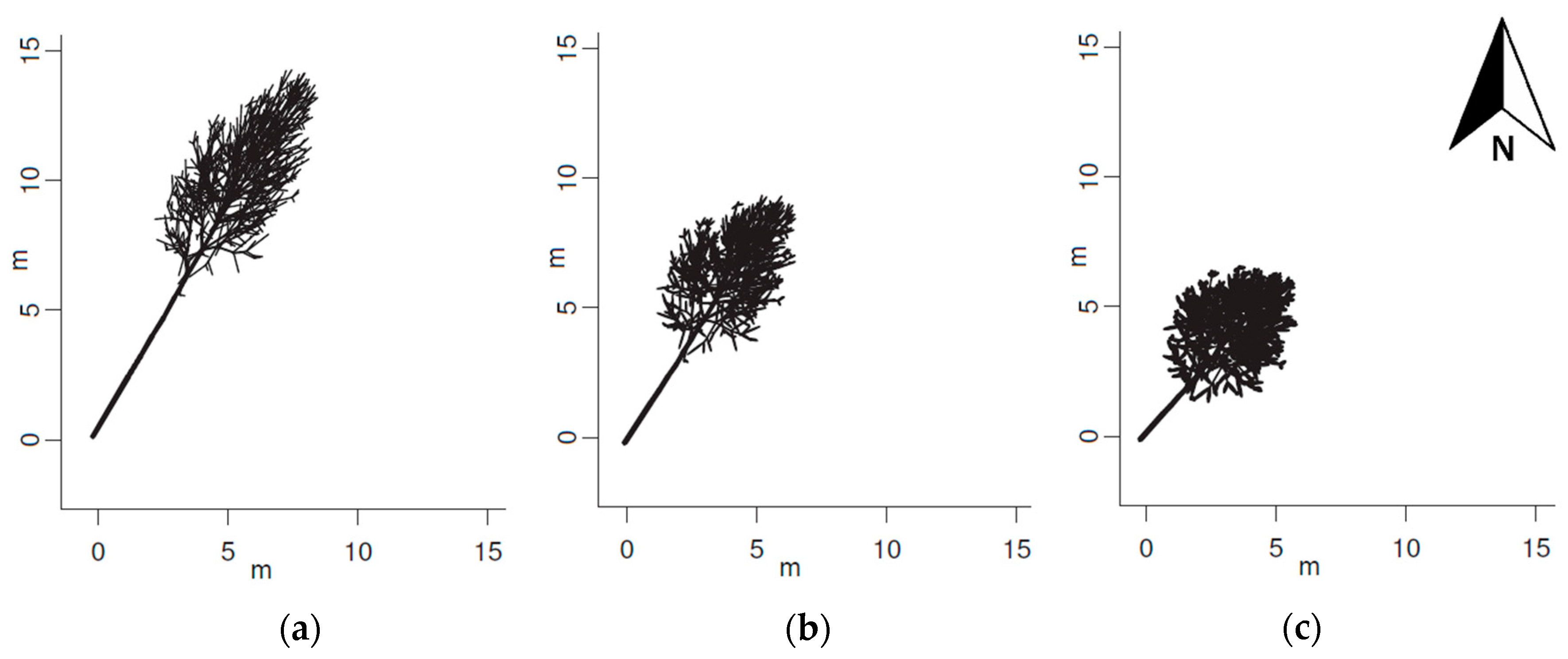
To simulate leaf growth, we let the minor axis radius of the ellipsoids increase during the vegetation period. It increases by 1 cm from April, starting with a radius of 2 cm, until July, then having reached a radius of 5 cm. From July to September, we assume the crown to be fully developed. In October, the leaves are shed, and the modeled tree enters the leafless stage. The projected shadows of the ellipsoids represent ellipses on the x-y-plane. Because the coordinates of the vertices of the ellipsoids are known, their shadow can be projected onto a shadow grid on the x-y-plane along with the shadows of leafless cylinders (Figure 3).

3. Results

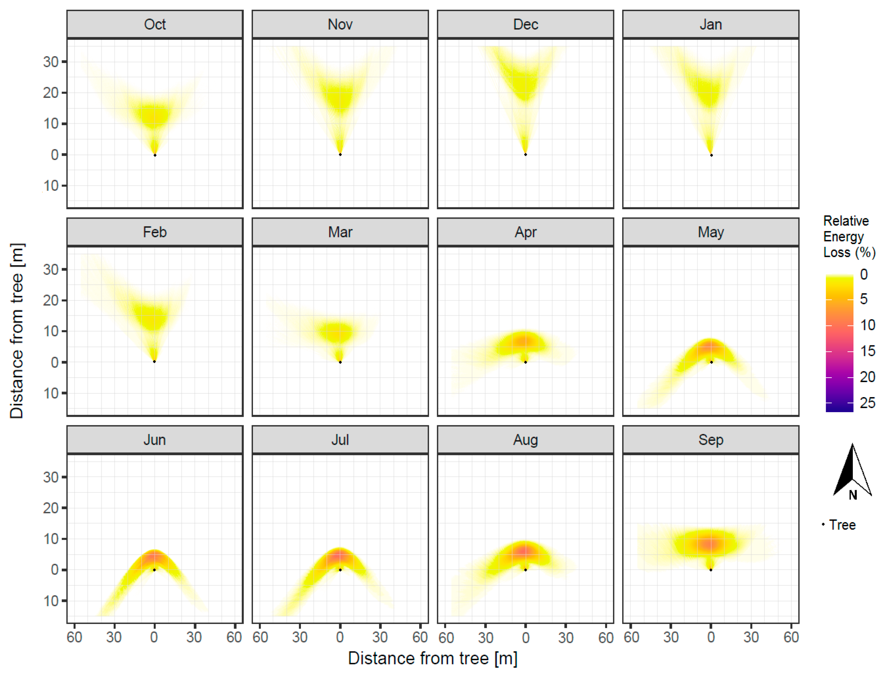
In this section, we present examples of visualized outputs of the developed shadow model. The daily shadow was modeled for one entire year, covering the time from 1 October 2013, until 31 September 2014. The starting date was set to October since the tree was scanned at that time being also the end of the vegetation period. We could subsequently assume no or minor changes on morphological attributes in the tree shape, leading to a realistic shading effect for this period. Figure 4 shows the shadow dynamics throughout this year in monthly sums. From October to March, the shading effect of the leafless tree is comparably weak, but it reaches areas in a distance of more than 30 m northward from the tree’s stem in a V-shape, especially in December. The shadow elongates until the time of the winter solstice and widens after passing this time of the year. In spring, the shadow of the tree crown moves closer towards the tree due to the sun’s shifting zenith positions, and it becomes increasingly intense due to the developing leaves. At the timings of the equinoxes, the shadow widens to a straight strip. In the period from June until September, the shadow is reaching the most intense and localized loss of solar energy on the ground and spreads in a hyperbole shape around the tree.
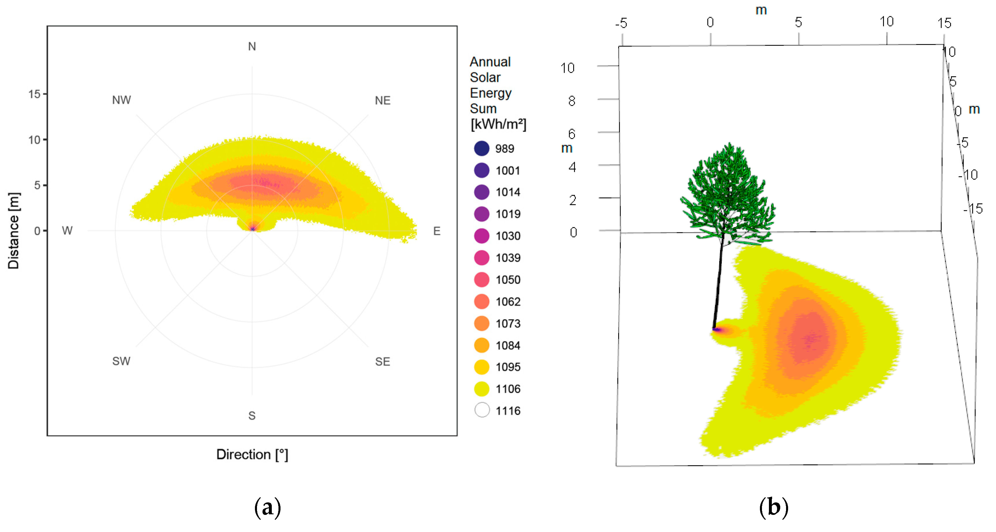
Figure 5a shows the annual solar radiation distribution below the model tree. The slightly asymmetrical shape of the cast shadow is due to the asymmetrical shape of the tree crown. The maximum annual solar radiation without shadow amounts to 1116 kWh m−2 (white area in Figure 5). The minimum annual solar radiation reaches 978 kWh m−2 in the area under the tree crown (dark area in Figure 5). The tree crown shading is most intense in the area around five to seven meters northwards from the stem.

4. Discussion

The presented model is the first 3D model of real trees that allows for a detailed temporal and spatial quantification of the solar energy losses beneath individual trees. Based on 3D cylinder models derived from TLS data, the model is able to compute the shadow projections of individual trees onto a raster with 10 cm × 10 cm cells on the ground surface exceeding other light models significantly.
Although the results displayed in these models show similarities with our model outputs, [6,7,11], even the more advanced versions work with coarser resolutions of 1 m2 grid cells [7,11] or 0.5 m × 0.5 m × 0.5 m voxels [9,13,16,24]. The high temporal resolution of 10-min intervals and the options to compute hourly, daily, weekly, monthly and seasonal dynamics of light availability at any geographical location provide the new option to study the changing patterns of interaction and competition for light of trees and understorey crops with an unknown accuracy.
The commonly used approach for modelling light availability, the turbid medium analogy, is assumed to underestimate low radiation values and to be unable to describe fine spatial patterns such as sun flecks since the crown architecture is not displayed precisely enough [25]. Models like the ellipsoidal crown approach, applying the turbid medium analogy [7,12], or the voxel approach [10,13,14] try to include the tree’s morphological features. A complicated but required step at this point would be the measurement and usage of the leaf area index (LAI) and/or the leaf area distribution (LAD) with uniform or random hypotheses for LAD. Yet, both hypotheses lead to an underestimation of shading between leaves and that there need to be further refinements in calculations when it comes to modelling light availability below single trees [7]. An important alternative approach has been introduced by [15], using a voxel-based light interception model by transforming the TLS scan of foliated trees into such small voxels, that mathematical corrections for the LAD became obsolete and values for LAD could be directly derived from TLS data. To avoid using estimated variables like the LAI, but to include the presence of crown gaps, we used a cylinder-based tree model that allows for introducing many small ellipsoids as leaf substitutes around the cylinders, rather than using only one single ellipsoid constructed around the entire crown.
Apart from the difficulty of realistically accounting for the individual trees’ crown architecture, the solar irradiance components constitute another critical issue when computing light availability in AFS. The total solar radiation on a horizontal area can be split up into direct irradiance and the diffuse irradiance, which is, besides the direct component, also important for the crops’ growth. Even if accurate and flexible solar mapping models based on LiDAR data exist [26], it was highlighted that most light availability models composed for tree and forest environments don’t account for the diffuse radiation [27]. The reviews of both light availability models and of solar mapping methods revealed that light models and solar maps are not realistic, and thus, not promising, if they are lacking information about diffuse radiation [24,28]. Our approach includes both components of direct and diffuse radiation, measured for every hour. However, the assumption that diffuse light is always completely present on the ground might lead to a slight underestimation of the shadow intensity [6,27]. Further, we assume that the spatial interpolation between the polygons of the 10-min time steps cannot completely account for temporal gaps, even though the energy amount lost through shading is adapted to 10 min. This could lead to a small but additional underestimation of the shadow intensity where an interpolation is performed (mostly along the lower stem shadow). Since other studies did not include the stem for shadow purposes at all [6], we need to compare this shading effect to future measurements of solar radiation on the research site and, if necessary, adjust the model appropriately.

5. Conclusions

Our model is a promising tool in quantifying and visualizing realistic light availability dynamics under a single tree—especially, since it allows for utilizing factual climate data that enable the realistic retrospective modeling of the radiation regime of a given tree and to quantify future developments based on these data. The usage of the terrestrial laser scanning method is a non-destructive tool for measuring tree volumetric data and collecting crown architectural information. Due to the option to retrospectively analyze the shadow cast by single trees and the high resolution solar radiation data, our vector-based approach results in lower labor costs and it reduces field work to a minimum of one scan per year to monitor tree growth. The results can be adapted in management decisions in AFS or similar land use systems. With the obtained information, whole systems and their planting design can be planned and optimized to minimize light loss for light demanding crop species. Furthermore, our model can help to identify the best tree/crop combination, so that crops adjusted to the present or desired light regime can produce the maximal yield.

6. Outlook

We show how the innovative utilization of high-resolution TLS-data can be employed to advance research in forestry and agricultural sciences using a model to derive information about the shadow cast by a single tree. However, this model needs to be refined and advanced along the following lines:
  • Improvement of the leaf simulations. Leaf parameters vary between tree species, within the tree crown and throughout the growing season [15,16,17]. Thus, to generate realistic shadow projections of tree crowns, it is crucial to simulate leaves as realistically as possible. At present, our model simulates leaves by adding a single ellipsoid to the end of branches of a radius of less than 0.5 cm, and the ellipsoids increase in their radius each month to simulate leaf growth. We will replace these ellipsoids with more realistic leaf-like polygons, taking also their spatial distribution within tree crowns into account.
  • Validation of the results generated by the model by comparing them with on-site light measurements. In case of discrepancies, the model needs to be adapted accordingly.
We are confident that these advancements can successfully be implemented, and that our model will serve as a useful tool that realistically describes the shadows cast by trees in AFS and other ecosystems in which their effects need to be better understood and quantified to improve their management.

Acknowledgments

The authors would like to thank Jan Hackenberg for his valuable support. This research was supported by the German Federal Ministry of Food and Agriculture (BMEL) within the projects Agro-Wertholz (support code 22031112) and SidaTim (support code 2815ERA04C). The article processing charge was funded by the Albert-Ludwigs-University Freiburg in the funding program open access publishing.

Author Contributions

E.R. and C.M. conceived and designed the experiments and the implementation; E.R. processed and analyzed the data and developed the model; E.R., C.M. and M.N. wrote the publication.

Conflicts of Interest

The authors declare no conflict of interest. The founding sponsors had no role in the design of the study; in the collection, analyses, or interpretation of data; in the writing of the manuscript, and in the decision to publish the results.

References

  1. Editors of Agroforestry Systems. What is Agroforestry? Agrofor. Syst. 1982, 1, 7–12. [Google Scholar] [CrossRef]
  2. Nair, P.K.R. An Introduction to Agroforestry; Kluwer Academic Publishers (in cooperation with the International Centre for Research in Agroforestry): Dordrecht, The Netherlands, 1993. [Google Scholar]
  3. Waggoner, P.E.; Pack, A.B.; Reifsnyder, W.E. The Climate of Shade, A Tobacco Tent and A Forest Stand Compared to Open Fields. Available online: http://www.ct.gov/caes/lib/caes/documents/publications/bulletins/b626.pdf (accessed on 24 May 2017).
  4. Muschler, R.G. Shade improves coffee quality in a sub-optimal coffee-zone of Costa Rica. Agrofor. Syst. 2001, 51, 131–139. [Google Scholar] [CrossRef]
  5. Stathers, R.J.; Bailey, W.G. Energy receipt and partitioning in a ginseng shade canopy and mulch environment. Agric. For. Meteorol. 1986, 37, 1–14. [Google Scholar] [CrossRef]
  6. Dupraz, C.; Liagre, F. Agroforesterie. In Des Arbres et des Cultures, 2nd ed.; Éditions France Agricole: Paris, France, 2011. [Google Scholar]
  7. Talbot, G.; Dupraz, C. Simple models for light competition within agroforestry discontinuous tree stands: Are leaf clumpiness and light interception by woody parts relevant factors? Agrofor. Syst. 2012, 84, 101–116. [Google Scholar] [CrossRef]
  8. Oker-Blom, P. Photosynthetic radiation regime and canopy structure in modeled forest stands. Acta For. Fenn. 1986, 197, 1–44. [Google Scholar] [CrossRef]
  9. Sinoquet, H.; Sonohat, G.; Phattaralerphong, J.; Godin, C. Foliage randomness and light interception in 3-D digitized trees: An analysis from multiscale discretization of the canopy. Plant Cell Environ. 2005, 28, 1158–1170. [Google Scholar] [CrossRef]
  10. Cifuentes, R.; Van der Zande, D.; Salas, C.; Tits, L.; Farifteh, J.; Coppin, P. Modeling 3D canopy structure and transmitted PAR using terrestrial LiDAR. Can. J. Remote Sens. 2017, 43, 124–139. [Google Scholar] [CrossRef]
  11. Artru, S.; Garré, S.; Dupraz, C.; Hiel, M.-P.; Blitz-Frayret, C.; Lassois, L. Impact of spatio-temporal shade dynamics on wheat growth and yield, perspectives for temperate agroforestry. Eur. J. Agron. 2017, 82, 60–70. [Google Scholar] [CrossRef]
  12. Stadt, K.J.; Lieffers, V.J. MIXLIGHT: A flexible light transmission model for mixed-species forest stands. Agric. For. Meteorol. 2000, 102, 235–252. [Google Scholar] [CrossRef]
  13. Oshio, H.; Asawa, T. Estimating the solar transmittance of urban trees using airborne LiDAR and radiative transfer simulation. IEEE Trans. Geosci. Remote Sens. 2016, 54, 5483–5492. [Google Scholar] [CrossRef]
  14. Dauzat, J.; Madelaine-Antin, C.; Heurtebize, J.; Lavalley, C.; Vincent, G. How Much Commercial Timber in Your Plot, How Much Carbon Sequestrated in The Trees, How Much Light Available for Undercrops? Terrestrial Lidar is The Right Technology for Addressing These Questions. Available online: http://agritrop.cirad.fr/580646/1/ID580646.pdf (accessed on 24 May 2017).
  15. Van der Zande, D.; Stuckens, J.; Verstraeten, W.W.; Muys, B.; Coppin, P. Assessment of light environment variability in broadleaved forest canopies using terrestrial laser scanning. Remote Sens. 2010, 2, 1564–1574. [Google Scholar] [CrossRef]
  16. Grau, E.; Durrieu, S.; Fournier, R.; Gastellu-Etchegorry, J.P.; Yin, T. Estimation of 3D vegetation density with Terrestrial Laser Scanning data using voxels. A sensitivity analysis of influencing parameters. Remote Sens. Environ. 2017, 191, 373–388. [Google Scholar] [CrossRef]
  17. Béland, M.; Widlowski, J.L.; Fournier, R.A.; Côté, J.F.; Verstraete, M.M. Estimating leaf area distribution in savanna trees from terrestrial LiDAR measurements. Agric. For. Meteorol. 2011, 151, 1252–1266. [Google Scholar] [CrossRef]
  18. Hackenberg, J.; Morhart, C.; Sheppard, J.; Spiecker, H.; Disney, M. Highly accurate tree models derived from terrestrial laser scan data: A method description. Forests 2014, 5, 1069–1105. [Google Scholar] [CrossRef]
  19. Morhart, C.; Sheppard, J.P.; Schuler, J.K.; Spiecker, H. Above-ground woody biomass allocation and within tree carbon and nutrient distribution of wild cherry (Prunus avium L.)—A case study. For. Ecosyst. 2016, 3, 1–15. [Google Scholar] [CrossRef]
  20. Hackenberg, J.; Spiecker, H.; Calders, K.; Disney, M.; Raumonen, P. SimpleTree—An efficient open source tool to build tree models from TLS clouds. Forests 2015, 6, 4245–4294. [Google Scholar] [CrossRef]
  21. Corripio, J.G. Insol: Solar Radiation. Available online: http://www.meteoexploration.com/R/insol/ (accessed on 24 May 2017).
  22. Deutscher Wetterdienst (DWD). CDC (Climate Data Center): Hourly Station Observations of Solar Irradiation. Available online: ftp://ftp-cdc.dwd.de/pub/CDC/observations_germany/climate/hourly/solar (accessed on 9 June 2017).
  23. R Core Team. R: A Language and Environment for Statistical Computing; R Foundation or Statistical Computing: Vienna, Austria, 2017. [Google Scholar]
  24. Zhao, W.; Qualls, R.J.; Berliner, P.R. Modeling of the short wave radiation distribution in an agroforestry system. Agric. For. Meteorol. 2003, 118, 185–206. [Google Scholar] [CrossRef]
  25. Meloni, S.; Sinoquet, H. Assessment of the spatial distribution of light transmitted below young trees in an agroforestry system. Ann. For. Sci. 1997, 54, 313–333. [Google Scholar] [CrossRef]
  26. Santos, T.; Gomes, N.; Freire, S.; Brito, M.C.; Santos, L.; Tenedório, J.A. Applications of solar mapping in the urban environment. Appl. Geogr. 2014, 51, 48–57. [Google Scholar] [CrossRef]
  27. Li, T.; Yang, Q. Advantages of diffuse light for horticultural production and perspectives for further research. Front. Plant Sci. 2015, 6, 704. [Google Scholar] [CrossRef] [PubMed]
  28. Freitas, S.; Catita, C.; Redweik, P.; Brito, M.C. Modelling solar potential in the urban environment: State-of-the-art review. Renew. Sustain. Energy Rev. 2015, 41, 915–931. [Google Scholar] [CrossRef]
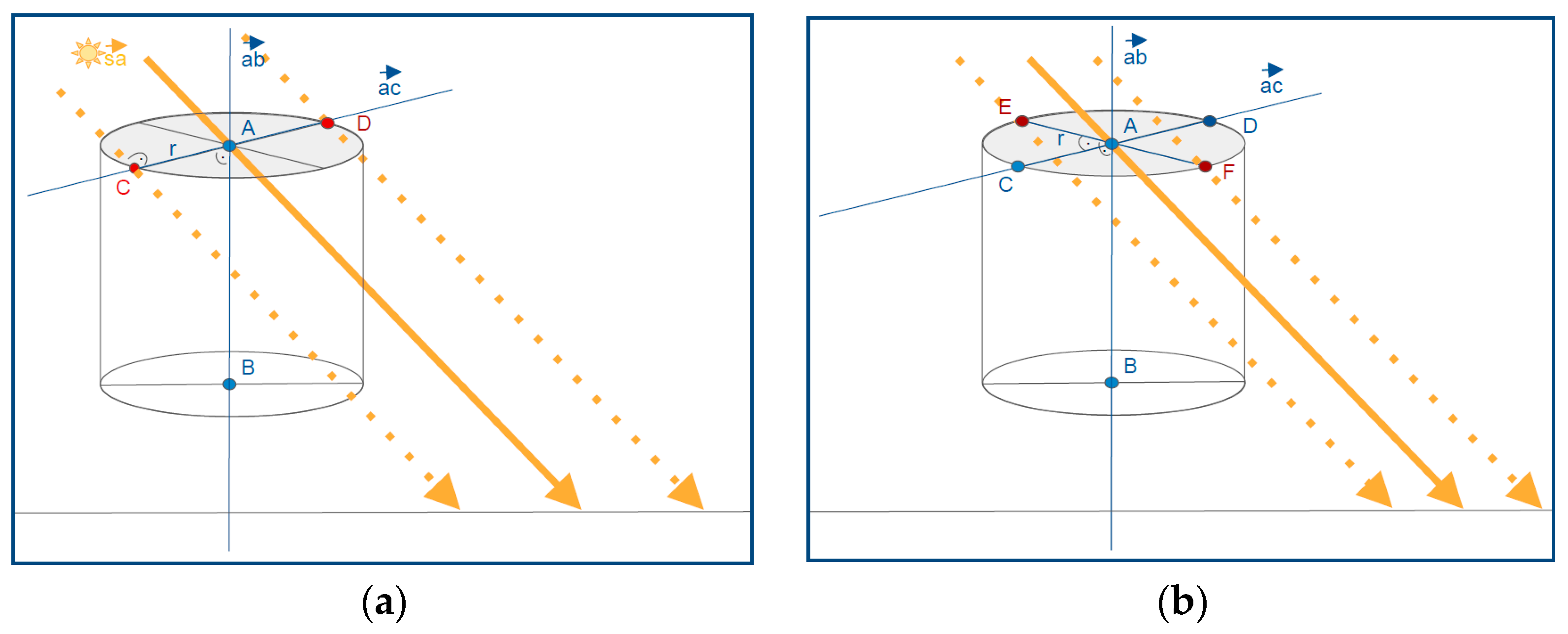
Figure 1. Cross product scheme: (a) The vectors s a (sun–center) and a b (center top–center bottom) must both be perpendicular to the new vector a c through the points C,D; (b) The vectors a c (center top–new point C) and a b (center top–center bottom) must both be perpendicular to the new vector a e through the points E,F.
Remotesensing 09 00719 g001
Figure 2. The 3D tree model (a) in the “leaf-off” mode; (b) in the leafy-ellipsoidal “leaf-on” mode (here shown with 5 cm width of the minor axis of the ellipsoid).
Remotesensing 09 00719 g002
Figure 3. The shadows of the tree model at three points in time with different stages of ellipsoids at 12:00 a.m.: (a) 15 March (no ellipsoids); (b) 15 April (2 cm ellipsoid width); (c) 15 July (5 cm ellipsoid width).
Remotesensing 09 00719 g003
Figure 4. Monthly grids of solar energy losses from October 2013 until September 2014 in comparison to unshaded areas.
Remotesensing 09 00719 g004
Figure 5. (a) Annual solar radiation distribution below the model tree along the compass directions, the outer circle representing a radius of 15 m around the tree stem; (b) the 3D visualization of the tree model with the annual solar radiation distribution.
Remotesensing 09 00719 g005