Article

Multiple Regression Analysis for Unmixing of Surface Temperature Data in an Urban Environment

Department of Environmental Sciences, University of Basel, CH-4056 Basel, Switzerland
*
Author to whom correspondence should be addressed.
Remote Sens. 2017, 9(7), 684; https://doi.org/10.3390/rs9070684
Submission received: 26 April 2017 / Revised: 16 June 2017 / Accepted: 30 June 2017 / Published: 4 July 2017

Abstract

:
Global climate change and increasing urbanization worldwide intensify the need for a better understanding of human heat stress dynamics in urban systems. During heat waves, which are expected to increase in number and intensity, the development of urban cool islands could be a lifesaver for many elderly and vulnerable people. The use of remote sensing data offers the unique possibility to study these dynamics with spatially distributed large datasets during all seasons of the year and including day and night-time analysis. For the city of Basel 32 high-quality Landsat 8 (L8) scenes are available since 2013, enabling comprehensive statistical analysis. Therefore, land surface temperature (LST) is calculated using L8 thermal infrared (TIR) imagery (stray light corrected) applying improved emissivity and atmospheric corrections. The data are combined with a land use/land cover (LULC) map and evaluated using administrative residential units. The observed dependence of LST on LULC is analyzed using a thermal unmixing approach based on a multiple linear regression (MLR) model, which allows for quantifying the gradual influence of different LULC types on the LST precisely. Seasonal variations due to different solar irradiance and vegetation cover indicate a higher dependence of LST on the LULC during the warmer summer months and an increasing influence of the topography and albedo during the colder seasons. Furthermore, the MLR analysis allows creating predicted LST images, which can be used to fill data gaps like in SLC-off Landsat 7 ETM+ data.

Graphical Abstract

1. Introduction

1.1. Motivation

A majority of the world’s population currently lives in urban environments. Data provided by the WHO predict that by 2050 this number will increase to almost 70% worldwide, reaching even higher numbers in more developed countries, which even today reach levels of 75% urban population (Switzerland, Germany, etc.) [1]. A huge part of the world’s population growth in the next 30 years will be concentrated in urban environments [2]. This increase in urban population is accompanied by huge problems affecting a large number of people, e.g., clean water supply, waste, energy, air pollution, and heat stress [3,4]. This last issue, only measurable at certain weather conditions with a complex measurement setup, is causing serious problems for human health, most obviously during severe heat waves [5,6]. Heat stress presents one end of the human thermal comfort scale and can cause large numbers of deaths in a short period. The summer of 2003 in Central Europe is a prime example of the potential effects of an extreme heat wave on human health. Long-lasting fair weather conditions due to persistent anticyclonic circulations, caused by large-scale circulation anomalies and historically low precipitation levels between May and August, were the major causes of this record-breaking summer in Europe [7]. More than 70,000 additional deaths occurred due to severe heat stress in Europe during the 2003 heat wave [8]. In summer 2015, Europe again suffered an extreme heat wave, resulting in an excess mortality of up to 30% in some regions [9]. Almost every year, severe heat waves are threatening specific parts of the world. Considering the Fifth Assessment Report of the Intergovernmental Panel on Climate Change (IPCC), such extreme events have increased since the mid-20th century and will be a usual phenomenon until the end of the 21st century [10]. Future heat waves are expected to be more intense, longer lasting, and/or more frequent [11,12]. Statistical analysis concerning the typical length of general weather situations supports these findings in Central Europe [13]. Human impact on the energy balance through enhanced urbanization, including the alteration of the physical surface properties and processes, intensifies this extreme heat stress [14,15,16,17]. The resulting increased air temperature in the urban canopy layer compared to its rural surroundings is often referred to as the urban heat island (UHI) [18,19,20]. For Basel, during the Basel Urban Boundary Layer Experiment (BUBBLE), the UHI phenomenon was investigated and described in detail [16]. An important finding during the BUBBLE campaign—which has also been mentioned in climate sciences before—is that the UHI effect is generally a nocturnal phenomenon, usually not measurable during the daytime, and that serious differences occur within different parts of the city, indicating several thermal zones. A total of 123 Tropical Nights (nocturnal Tmin > 20 °C) and 26 Extremely Hot Days (Tmax > 35 °C)—examples of days with extreme heat stress—were measured in the last 15 years at an urban measurement tower in Basel, most of them during the summers of 2003 and 2015. Studies on the urban climate have a long tradition in climatology [21,22,23] and emphasize the clear tendency of enhanced heat stress within cities, e.g., [16,18,24,25]. Regarding the growing urban population and therefore increasing city size, combined with the increasing number of heat waves expected in the near future, the study of urban climate with a focus on human thermal comfort is inevitable for future urban planning. Nevertheless, the understanding and integration of this issue in urban planning is still expandable [24,26].

1.2. State of the Art

To investigate large-scale urban climate characteristics, remote sensing in its various forms offers great opportunities with lots of benefits, but also challenges to comprehend. Geostationary satellites, polar orbiting satellites, airborne platforms, and considerably improved UAVs offer manifold possibilities to observe the Earth’s surface in different spatial, spectral, and temporal resolutions. One of the main challenges in urban remote sensing is the conversion of large-scale two-dimensional measurements into meaningful and useful information for dwellers and urban planners. Besides the challenges to conquer the scale limitations, remote sensing data—especially TIR data—are seriously affected by atmospheric effects, mainly by water vapor and ozone, or instrumental problems. The latter can cause severe errors in absolute values and is difficult to compensate for, e.g., the L8 Thermal InfraRed Sensor (TIRS) stray light issue discussed in Section 1.3. Atmospheric effects due to attenuation and enhancement of the emitted signal are inevitable and well known. To counteract these limitations, numerous investigations have been conducted [27]. Crucial findings considering the application of TIR remote sensing in urban environments were reported by Voogt and Oke in numerous studies, e.g., [28,29,30]. Theoretical background, several problems and recent developments in this field are summarized in detailed reviews by [31,32,33]. As a practical application, Dousset et al. (2011) have demonstrated the use of satellite data for monitoring the 2003 heat wave in the metropolitan area of Paris. Due to their findings, the severity of future heat waves can be better predicted through analysis of vegetation dynamics, and the contribution of the UHI to raising minimum nocturnal temperatures—linked with heat stress and mortality—was elaborated [34]. In other studies, the use of multitemporal data from multiple sensors enables the investigation of statistical trends and the modeling of annual cycles [35] or performing disaggregation of LST through thermal sharpening, temperature unmixing and/or data fusion [36,37,38,39,40] to improve the temporal and spatial resolution. Thereby, the use of different datasets with dissimilar viewing directories on the target is a possible source of error and has to be interpreted with caution, because sunlit or shaded surfaces may be overrepresented by certain viewing angles and/or off-nadir perspectives [41]. Different studies have focused on the estimation of soil moisture or evapotranspiration using TIR remote sensing and vegetation cover, combined with in situ measurements [32,42,43].
However, the simplicity of using remote sensing data has often led to misunderstanding and misinterpretation of TIR data. Therefore, one should clearly distinguish between the UHI considering the ambient air temperature in and above the canopy layer, and the two-dimensional surface urban heat island (SUHI) describing the urban surface temperature retrieved from remotely sensed TIR data [17]. During cloud-free days, the diurnal LST is usually several degrees higher than the ambient temperature and the LST patterns do not necessarily correspond to the ambient temperature patterns during the day [44]. In Basel, the SUHI can be found during both day and night, but the UHI is typically more pronounced during the night [16,17,18,19,20].

1.3. Problems with Thermal Infrared Data

The abundance of two TIR channels for L8 would offer the possibility of using a split window algorithm (SWA), comparable to ASTER applications [33,45]. Due to stray light anomalies within the two thermal bands of the TIRS, the U.S. Geological Survey (USGS) advised users to work only with TIRS band 10 with lower expected errors compared to band 11 before 24 April 2017 [46,47]. In the meantime, NASA recomputed all L8 TIR data according to the algorithm of Gerace and Montanaro (2017), which reduces the error of both TIR bands to less than 1 K [48]. This paper makes use of the stray light corrected L8 TIR data. Nevertheless, NASA recommends not using SWA for atmospheric correction [49]. Therefore, it is still necessary to use radiative transfer models such as MODTRAN [50,51,52,53] to remove the atmospheric effects occurring between the Earth’s surface and the satellite sensor. These models simulate the attenuating and enhancing effect of atmospheric gases and aerosols on the TIR signal and are used to convert the at-sensor or top-of-atmosphere (TOA) radiance to surface-leaving radiance. Numerous studies use standard atmospheres in MODTRAN to correct TIR data. However, a more sophisticated approach is the use of spatiotemporally interpolated data providing atmospheric global profiles for a particular date, such as the National Center for Environmental Prediction (NCEP) reanalysis model to simulate the atmospheric conditions on a global scale. This data is available in a six-hour frequency for atmospheric conditions since the year 2000 to get a better simulation of the atmospheric conditions during the satellite overpass [54,55]. The most convenient way to combine this reanalysis data with MODTRAN code is the web-based atmospheric correction tool (ACT) provided by NASA and developed by Julia Barsi [56,57]—accessible on www.atmcorr.gsfc.nasa.gov.
The two-dimensional TIR data are an extremely useful measure and provide information on a large scale that is easy to access and easy to use. Compared to point measurements obtained from measurement towers or stations, there are some disadvantages to using remote sensing data as well. The low temporal resolution of polar orbiting satellites leads to TIR data showing just a snapshot of the actual properties at a specific time of day.
Furthermore, only fair weather conditions are investigated, and therefore the results are only valid for clear-sky days.

1.4. Research Questions

The question of this investigation is not whether there is a SUHI available, but more what the distribution looks like in different parts of the city and, furthermore, how it can be explained by surface properties. In the scope of this paper, a large satellite dataset is used to find significant tendencies in LST dynamics with seasonal variations and to investigate the connections to the land cover. Careful atmospheric corrections and emissivity estimations are developed to generate a proper data basis. The reliability of the data is one important point for discussion. Thereafter, statistical analysis is first developed for administrative subunits to reveal trends and demonstrate the connection between LULC and LST within residential units.
To quantify the effect of land cover on LST and reveal the seasonal distribution, a MLR approach—inspired by spectral unmixing—is developed and applied on bulk data. Spectral unmixing is a method developed for the decomposition of mixed pixels using linear regression, linear mixture models or neural networks applied on hyperspectral data [58]. Deng and Wu (2013) have used spectral unmixing to derive fractional urban compositions and used the results to predict TIR data based on the thermal responses of these compositions and their abundances [59]. Applying this scheme, thermal endmembers derived from ground station TIR measurements are used to simulate LST for the whole study area, even during days with comprehensive cloud cover [60]. Other studies used empirical measurements to convert land-cover-specific surface temperatures to land-cover-specific air temperatures applied on mixed pixels to predict the pixel average air temperature [61]. In this study, a related approach was developed where the abovementioned spectral unmixing is replaced by mixing various surface characteristics (i.e., land cover fractions, vegetation cover, albedo, and solar irradiance sum) to a coarser resolution (100-m cells). These input data are used in a MLR analysis to predict the LST, based on the actual LST as the response. The resulting coefficients of the MLR analysis describe the effect of the predictors on the LST signal throughout the whole scene. The method is applied on a large dataset with chronologically variable data including clear sky days only and covering all seasons.
To understand the seasonal dynamics, simple linear regressions between vegetation cover and LST are included as an additional evaluation.

2. Materials and Methods

2.1. Data

The TIR data converted to LST have been acquired by the TIRS on board of the L8 satellite orbiting the Earth since March 2013. Due to the overlapping paths 195 (scene center) and 196 (right margin), a large number of suitable scenes (i.e., 32) with zero or nearly zero cloud cover (masked) and haze or fog (not used) could be found within four years of orbiting time. Only two scenes show more than 0.5% cloud cover, which was not covering the urban areas and therefore the data were nevertheless used for the study after masking. Atmospheric effects on the TIR signal are highly dependent on total column water vapor (TCWV) [62]. During all acquisitions, the TCWV did thereby not exceed 2.5 cm and a majority of the scenes was acquired with a TCWV below 1.5 cm. For the atmospheric correction, NCEP reanalysis data accessed via the web-based ACT [56] and improved with in-situ meteorological data from a measurement tower—maintained by the Research Group of Meteorology, Climatology and Remote Sensing of the University Basel (MCR)—is applied [63]. The data is adapted to terrain by the ASTER Global Digital Elevation Model (GDEM). Since the ACT only provides correction factors for the TIR channel, the visible (VIS), infrared (IR), and shortwave infrared (SWIR) channels are not corrected for atmospheric effects.
The LULC map has been developed in a previous study and is based on multitemporal L8 data from the years 2013 to 2015 with 15-m (pan-sharpened) spatial resolution (Figure 1) [64].
To analyze the data in specific scales and enable comparisons to demographic statistics, residential units provided by the Canton of Basel-Stadt (BS) are used [65].
The datasets were delivered with different geographic coordinate systems. To maintain the reliability of the measured data and ensure the comparability of the different datasets, the native coordinate system UTM-32N of the L8 scenes is used continuously. All data used in this study are summarized in Table 1.

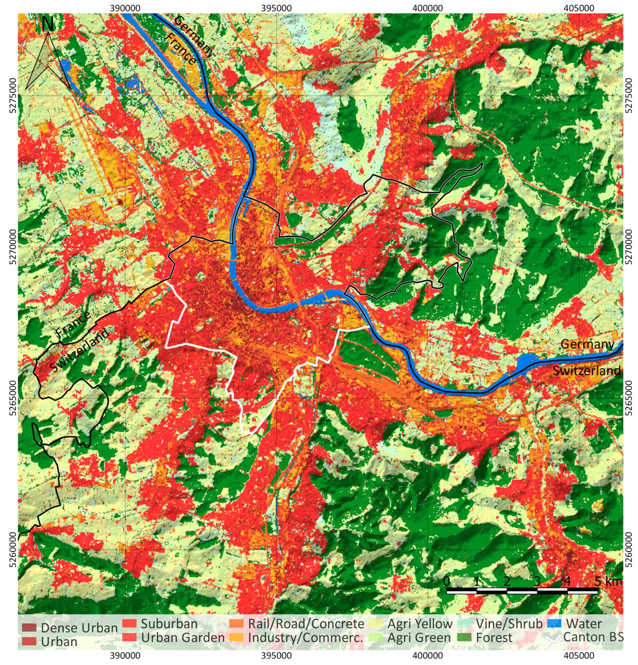
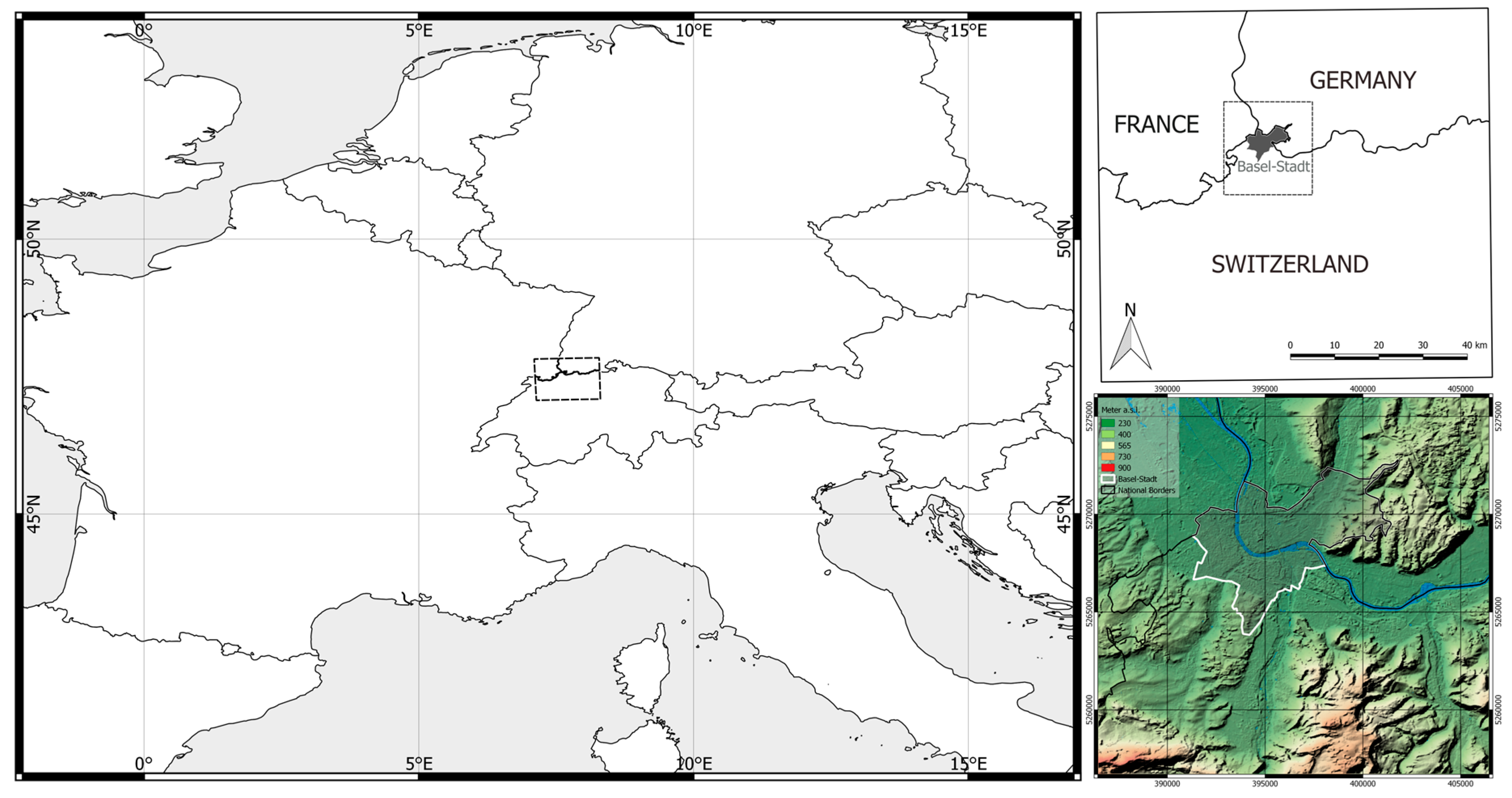
2.2. Site Description

Basel is located at the southern end of the Upper Rhine Valley between the bordering hills of the Vosges (France), the Black Forest (Germany), and the Jura Mountains (Switzerland) at about 250 m a.s.l. with a distinct topography (Figure 2).
The climate is considered oceanic, with mild winters and warm and sunny summers (Köppen Cfb climate) [26,66]. The annual mean temperature is 10.5 °C with an annual precipitation rate of 842 mm according to the suburban weather Station Basel/Binningen maintained by the Federal Office of Meteorology and Climatology for the reference period 1981 to 2010 [67]. Due to the suburban character of the measurement site surrounded by a large green space and situated on a moderately elevated hill, the typical urban annual mean temperatures of Basel can be considered some tenths of a degree higher due to higher nocturnal minimum temperatures [16]. The warmest month is usually July with mean temperatures above 25 °C, even though record-high temperatures during heat waves are usually favorable in August. During the BUBBLE project in 2005, a distinct nocturnal UHI was found for Basel, even if the surrounding hillsides with large forests supply the city with fresh air due to nocturnal cooling and cold air production [16]. Often, this cold drainage flow is only measured in rural or suburban stations surrounding the city. Combining these different measurement stations, daily and continuous UHI monitoring is implemented and publicly available (www.mcr.unibas.ch).
The investigation area contains the metropolitan area of Basel with approximately 730,000 inhabitants in total, including the bordering suburbs located in the Canton of Basel-Land (BL), the German cities Weil-am-Rhein and Lörrach, the French city Saint-Louis, and the city of Basel [26,68]. From north to south and west to east the area measures 21 by 20 km2, respectively, spanning from the upper left (47°38′35′′N, 7°29′17′′E) to the lower right (47°27′25′′N, 7°45′32′′E).

2.3. Methods

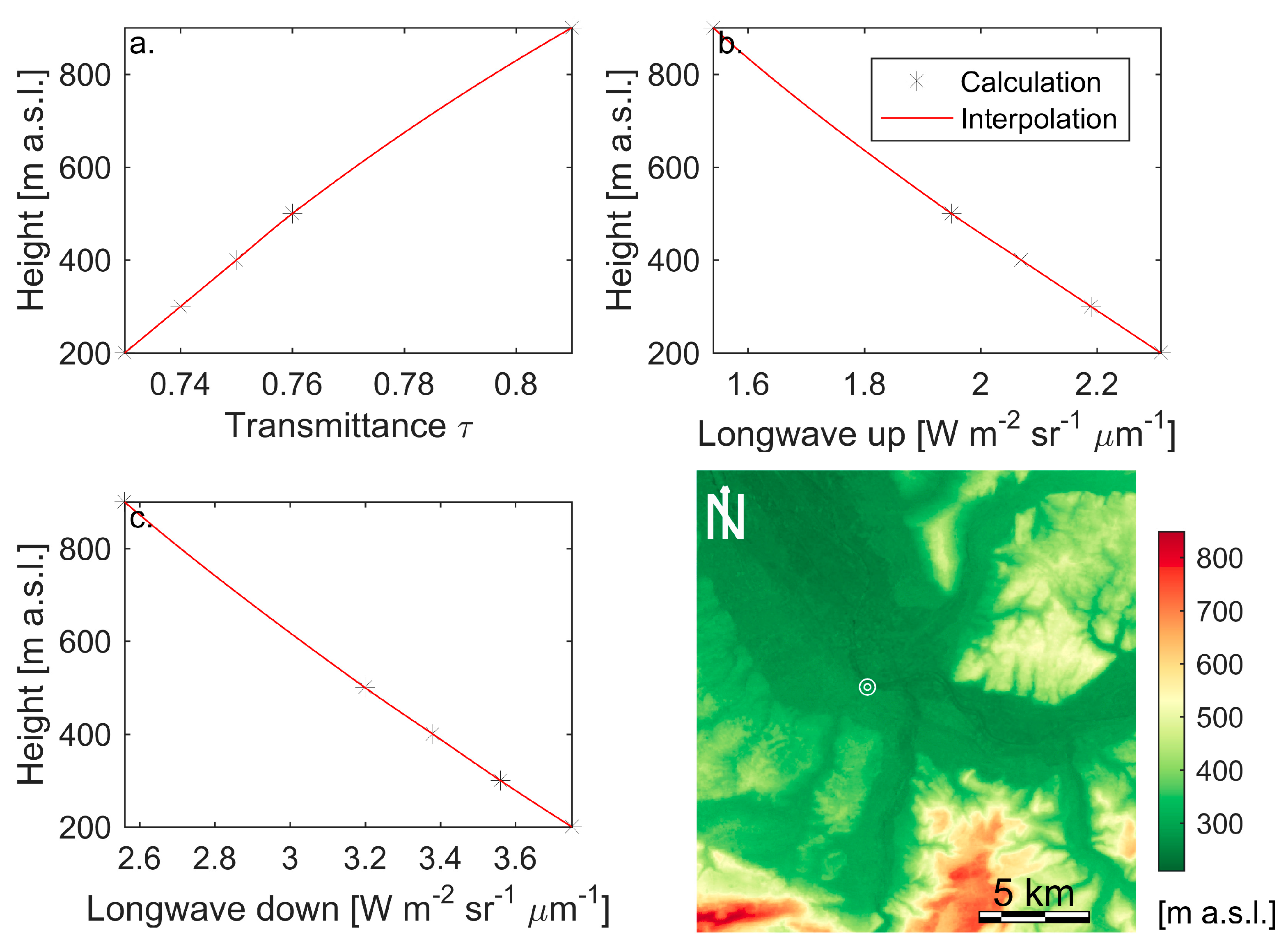
2.3.1. Land Surface Temperature

The atmospheric correction is done using the ACT provided by NASA [56,57] to receive the transmissivity, the longwave upwelling or atmospheric path radiance and the longwave downwelling or sky radiance for the correction of atmospheric effects on the surface-leaving TIR signal [69]. The ACT generates these parameters for a single point representing the whole scene, which is inadequate in the case of considerable elevation change. Thereby, an automated query on the ATC is collecting atmospheric correction parameters for different ground heights. These values are projected to the underlying topography using a piecewise cubic interpolation (Figure 3). Meteorological ground truth data from the measurement station Basel Klingelbergstrasse [63] representing the surface conditions (i.e., relative humidity, air temperature, and pressure) are implemented directly from the local database to improve the model. The adaption to the topography is applied because the biggest part of the atmospheric effect on the TIR radiation occurs in the planetary boundary layer, typically the thickest part of the atmosphere where most of the gases and aerosols are concentrated. The investigation area includes elevations of 250 m a.s.l. in the lower parts of the Rhine valley and almost 900 m a.s.l. in the Jura hills. Especially during stable anticyclonic conditions, a typical weather situation for proper remote sensing data acquisition, distinct differences in atmospheric conditions between the valley boundary layer and the surrounding hillsides are expected.
The differences are taken into account calculating the atmospheric correction parameters to receive surface-leaving radiance ( L T ) from TOA radiance ( L λ ) using Equation (1):
L T   =   τ ε L λ   +   L u   +   τ ( 1   -   ε ) L d ,
with transmissivity ( τ ), longwave upwelling ( L u ) and longwave downwelling radiance ( L d ). L T   is corrected using an emissivity map ( ε ), created after a modified vegetation-threshold approach by Sobrino (2008) [70] using the normalized difference vegetation index (NDVI) as a major criterion [42,71,72]. The natural deviation water index (NDWI) and the natural deviation built-up index (NDBI) are used as additional criteria to improve the reliability of the emissivity map because the NDVI threshold method is originally developed for rural areas [73,74,75,76,77]. These indices use normalized ratios in the VIS, NIR and SWIR range (subscript numbers describe the center wavelengths), explained in Equation (2a)–(2c):
NDVI   =   NIR 0.86   -   VIS 0.65 NIR 0.86   +   VIS 0.65 ,
NDWI   =   VIS 0.56   -   NIR 0.86 VIS 0.56   +   NIR 0.86 ,
NDBI   =   SWIR 1.61   -   NIR 0.86 SWIR 1.61   +   NIR 0.86 .
The use of indices for highly sealed and water surfaces is necessary due to the bad performance of the NDVI method on concrete surfaces or surfaces with negative NDVI values such as water [78]. Thereby, fully vegetated pixels with a NDVI > 0.5 ( NDVI V ) received an emissivity value of 0.99 ( ε V ); pixels with a NDWI ≥ 0 received an emissivity value of 0.98 for water surfaces. Soil pixels with a NDVI < 0.2 ( NDVI S ) are set to an emissivity value of 0.97 ( ε S ) [70,79,80]. Explicit built-up areas with a NDBI value > −0.2 and a seasonally maximum NDVI ≤ 0.35—obtained by analyzing multitemporal L8 scenes to omit false classified soil surfaces, which are not always separable from urban areas in a single-scene NDBI analysis—received an emissivity value of 0.9612. This number is estimated through averaging of typical emissivity values for asphalt, concrete, asphaltic concrete, construction concrete, and red brick based on the ASTER spectral library [80]. These materials represent the average urban surfaces of Basel to a large amount.
The remaining pixels, i.e., pixels with NDVI values between 0.2 and 0.5, are classified according to Equation (3) [70]:
ε   =   ε V P V   +   ε S ( 1   -   P V )   +   C .
The vegetation portion P V   is defined through the individual NDVI values and the threshold values NDVI S (0.2) and NDVI V (0.5) (Equation (4)), and C is defined as the cavity effect (Equation (5)):
P V   =   ( NDVI   -   NDVI S NDVI V   -   NDVI S ) 2 ,
C = ( 1 - ε s ) ε v F ( 1 - P v ) ,
with the geometrical factor F (i.e., shape factor) ranging from zero to unity, depending on the surface geometry. In this case, F is not automatically definable through optical or TIR data. Therefore, a mean value of 0.55 is chosen, as proposed by [81].
Surface leaving radiance in Wm - 2 sr - 1 μ m - 1 is converted to LST in Kelvin using the inverse Planck equation, or the Landsat specific estimate of the Planck curve, explained in Equation (6):
T   =   k 2 ln ( k 1 L T   +   1 ) ,
where T is the LST and k 1 and k 2 are calibration constants given for the sensor by the L8 metadata [82].

2.3.2. Land Use/Land Cover

The LULC map was created during earlier work described in Wicki and Parlow (2017) [64]. The approach is based on multitemporal L8 images from the years 2013 to 2015 considering only scenes in June, July, and August to guarantee comparable sun elevation and vegetation cover. Seven different classifications using training areas and a Maximum Likelihood Classifier were combined through a modal algorithm to create one accurate land cover map, shown in Figure 1.

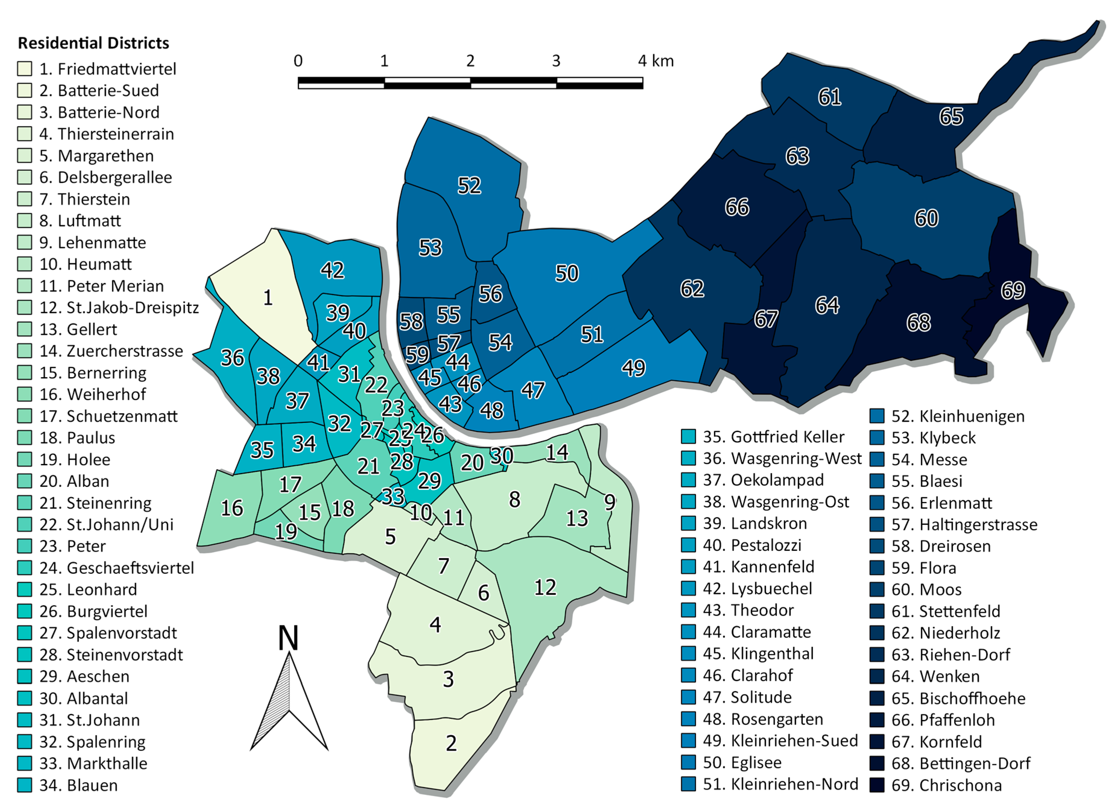
2.3.3. Administrative and Residential Boundaries

To aggregate the data reasonably, GIS data provided by the administration of BS is used. This dataset includes statistical residential units in three different scales of neighborhoods (different neighborhoods of the city of Basel and the community limits of the surrounding villages, which are part of BS), residential districts (neighborhoods subdivided into subunits, Figure 4), and residential blocks (typically housing blocks divided by streets).
In this work, only the results from the residential units are shown, because they reveal the best trade-off between uniform surface cover, size, and manageable quantity. Because the residential data is only available for the administrative area of BS, the MLR is performed in a simple 100 by 100-m2 raster on the entire investigation area.

2.3.4. Averaging Land Surface Temperature and Spatial Land Cover Fractions

The residential units are used as reasonable subdivisions to generate significant averaging in accordance to the urban morphology. The averaging (Equation (7)) is done with a simple loop over the numbers of patches based on the specific ID (n) given by the source data and for all available scenes (s).
avg n s =   LST ¯ x , y = n s
The calculated values are displayed in a map using the specific ID of the individual patches to address the pixels within the raster. The LULC is also analyzed patch-specific, giving each patch the total land use percentage—similar to the LST averaging—using the patch ID. This allows addressing each residential district concerning the connection between the percentages of LULC and the seasonal LST variations.

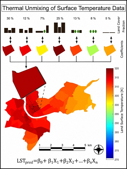
2.3.5. Multiple Linear Regression Analysis

A MLR analysis is used to decompose the thermal signal based on several input predictors. Thereby, the dependence of LST on surface cover and solar irradiance is computed using a LULC analysis, spectral indices (i.e., albedo and NDVI) and the sum of the total solar irradiance integrated from sunrise until the time of the satellite overpass.
The LULC and LST data is resized to 100 m pixel resolution, giving each pixel the mean LST and the land cover fraction. To reduce the number of predictors, related LULC classes are aggregated (i.e., Agriculture/Lawn = Agriculture Green + Agriculture Yellow, Suburban = Suburban + Urban Garden, Industry/Commercial = Industry/Commercial + Rail/Road/Concrete).
As a seasonal component, NDVI and albedo where included in the model as well. The NDVI is explained in Equation (2a) as a normalized ratio between the reflectance bands of the red and near infrared channels. The land surface broadband albedo is estimated after an approach by Liang (2001) using the calibrated reflectance of five channels from the VIS to the SWIR range ( ρ 2 7 ) as a weighted average in Equation (8) [83]:
a short   =   0.356 ρ 2   +   0.130 ρ 4   +   0.373 ρ 5   +   0.085 ρ 6   +   0.072 ρ 7   -   0.0018 .
The digital numbers (DN) are converted to TOA reflectance by using gain and offset from the L8 metadata to generate TOA radiance ( L λ   in   Wm - 2 sr - 1 µ m - 1 ), shown in Equation (9):
L λ   =   gain * DN   +   offset .
Thereafter, solar exoatmospheric irradiance ( E λ ), sun elevation ( Θ ) and Earth-Sun distance ( d ) are used in Equation (10) to create TOA reflectance ( ρ λ   unitless from zero to unity) for each band ( λ ):
ρ λ = π L λ d 2 E λ sin Θ .
If the reflectance gain and offset are available, the TOA reflectance can be directly calculated using these values, similar to Equation (9), with additional scaling by the sine of the sun elevation.
The total solar irradiance for the whole investigation area is modeled using a modified shortwave irradiance model (SWIM) [84]. SWIM uses a DEM and the respective topographic parameters (i.e., slope and aspect) to compute the shortwave incoming radiation at a specific day of the year (DOY) and a specific time of the day, taking into account different sun azimuth and elevation, sun’s declination, and atmospheric scattering processes. To generate the total sum of irradiance, which is relevant because the soil stores energy and therefore has a thermal history, the solar irradiance is iteratively modeled in six-minute steps from sunrise to the time of satellite overpass at the specific DOY and summed up.
The MLR model returns a vector of coefficient estimates for a multilinear regression of the responses (i.e., LST) on the predictors (i.e., land cover fraction, spectral indices and sum of solar irradiance) and an intercept value, which is the expected value when the predictors are set to zero and close to the average of the scene. To keep the outputs realistic, the response data is often centered, which returns an intercept of zero. In this case, the intercept serves as an orientation about the average LST values and the response data is therefore not centered or normalized. Unlike for the predictors, which had to be normalized to enable a homogeneous display due to their large differences in scale (e.g., NDVI has a range of minus one to unity and solar irradiance sum is a physical quantity in the range of 1 to 10 MJm−2). The predictors, measured/modeled/computed in different scales, are adjusted to a notionally common scale with values ranging from zero to unity. Regardless whether the response variable or the predictors are normalized or centered, the correlation coefficient is not altered at all. Only the coefficients of the individual predictors have to be interpreted with respect to the scaling. Applying the resulting regression formula (Equation (11)) for every scene in a two-dimensional pixel environment, a predicted LST image ( LST pred ) can be produced:
LST pred ( x , y )   =   β 0 ( x , y )   +   β 1 X 1 ( x , y )   +   β 2 X 2 ( x , y )   +     +   β n X n ( x , y ) ,
with the intercept as β 0 , the individual coefficients as β 1 n , and X 1 n as the input predictors. The model is run for every individual scene using bulk processing, which returns a matrix of coefficients for every predictor and every individual scene and statistical characteristics to assess the success of the model.

3. Results

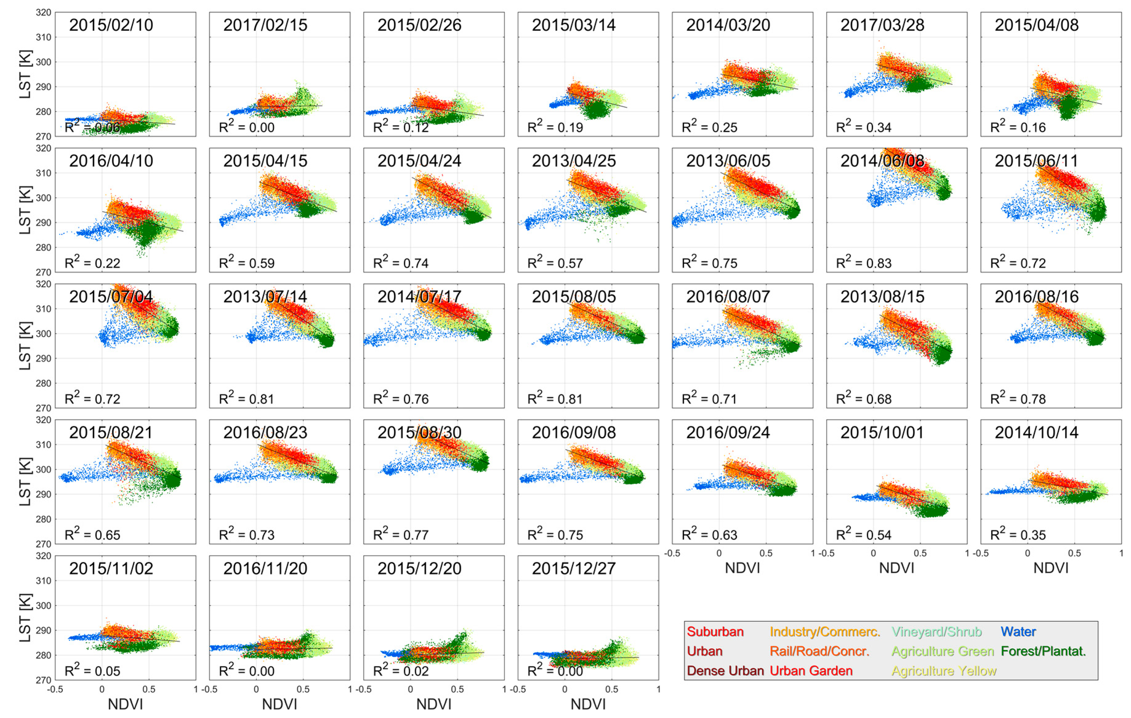
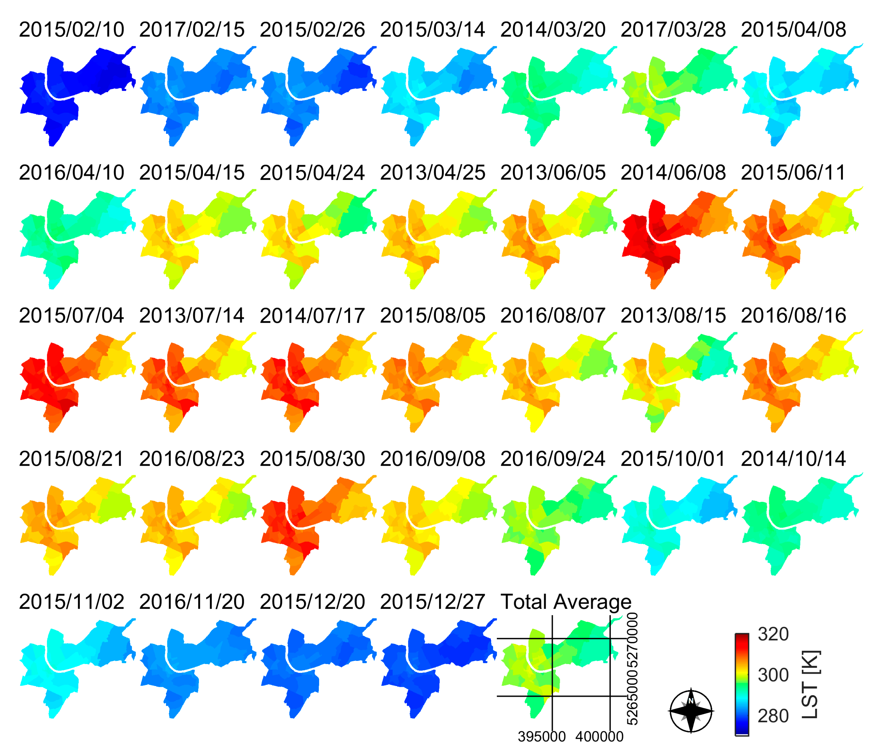
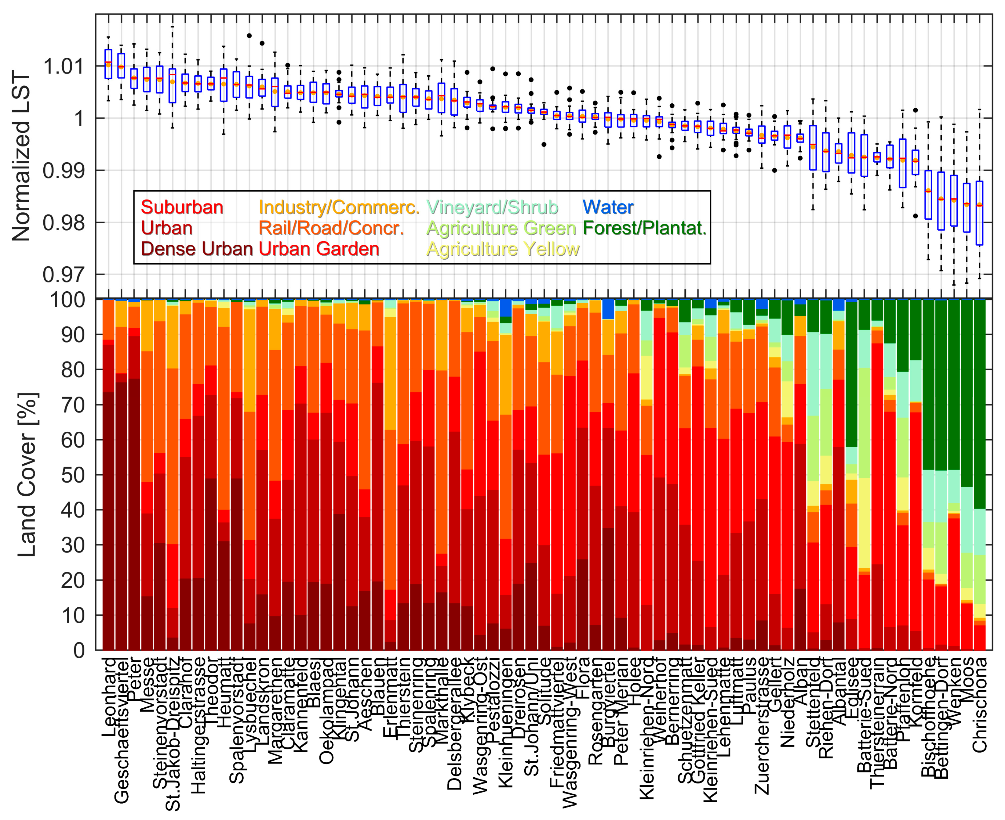
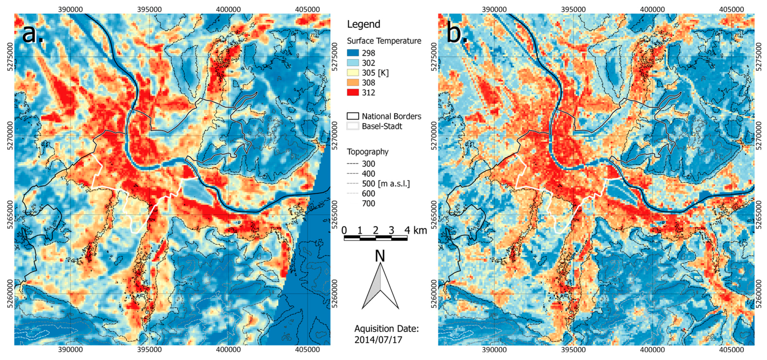
3.1. Land Surface Temperature and Land Use/Land Cover

The LST averaging within different residential districts shows the seasonal variations and the systematic distribution of hot spots or colder areas within the BS extent (Figure 5). The variation of LST within the different parts of the city is striking and seems to be stable despite large seasonal changes.
The LULC map is used to determine the portion of the different LULC classes in the residential district patches. This allows for identifying the different LULC distribution and comparing the resulting LST arranged as total averages. To omit seasonal effects and ignore possible temperature bias, the individual average temperatures of the patches are normalized to the individual mean of the entire scene. Combined with a bar plot summing up the different class percentages of each residential district, the urban characteristics supporting high LST become apparent since the districts are ordered after the descending seasonally mean LST (Figure 6). Results are only shown for the residential districts, because the spatial distribution looks familiar in both residential units, but the neighborhood unit consists of much more aggregation of surfaces that should be separated. Therefore, residential units are found to be a useful scale for urban climate analysis.
The highest LST are measured in districts with a dominance of the Dense Urban land use type, but also the combination of Dense Urban, Urban and Rail/Road/Concrete seems to produce high LST. However, even similar LULC combinations can cause different LST distributions: Besides the old town districts consisting of more than 70% Dense Urban, the almost purely industrial site St. Jakob-Dreispitz is one of the hot spots within the city. The structurally similar Erlenmatt district at the other end of the city is ranked far behind, indicating local effects. Regions consisting of high amounts of urban or industrial surfaces show lower LST if some percentages are counted to the water class, even if there are no—or only a few—natural surfaces detected (e.g., Burgviertel or Albantal). Seven out of 10 districts with the lowest LST show a LULC distribution of at least 50% natural surfaces; four out of five districts with the lowest LST consist of about 80% natural surfaces with each containing at least 50% forest pixels. Additionally, these districts with a high amount of natural surfaces also show the highest seasonal variability. Districts with a dominance of the class Suburban are usually found at the lower end of the descending LST scale. Thereby, industrial classes do not automatically involve high LST: Erlenmatt consists of about 80% industrial surfaces (Rail/Road/Concrete plus Industry/Commercial) with only 5% natural surfaces, but the average LST is lower than in many typical residential areas and ranks closer to the middle than to the top of the LST distribution table.

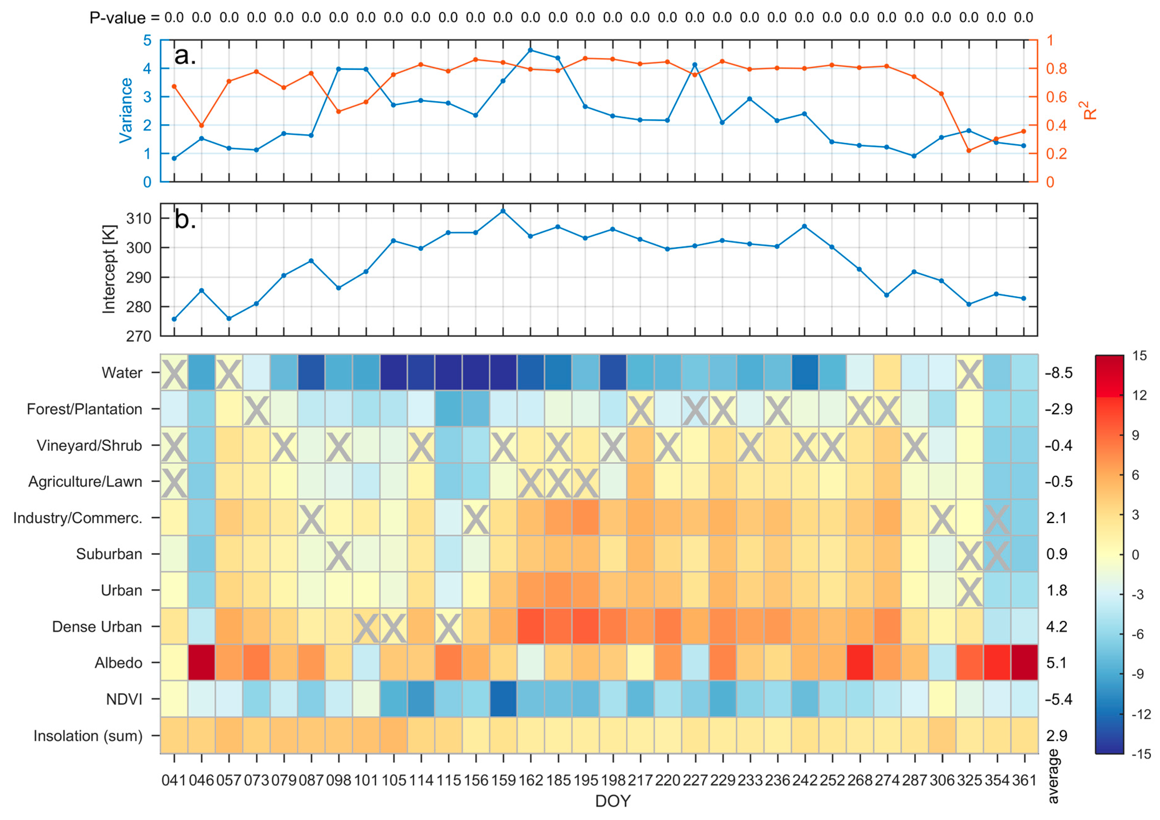
3.2. Multiple Linear Regression Analysis

A MLR analysis is used to describe LST (i.e., the response) by land cover fractions, spectral indices and the solar irradiance sum (i.e., the predictors) in a 100-m raster for all scenes. The models show R2 values between 0.75 and 0.87 in the warmer and highly vegetated periods of the year (i.e., DOY 105 to 287), meaning 75% to 87% of the LST distribution is explained by the predictors with overall p-values below 5% for all runs, indicating high significance. The resulting coefficients describe the increasing or decreasing effect of each variable on the LST in every scene (Figure 7). Thereby, not every predictor contributes always to an improvement of the multiple regression analysis. Individual predictors falling below the 5% benchmark for the p-value are flagged with gray crosses in Figure 7. However, the omission of these predictors did not affect the correlation factors dramatically and all regression runs are carried out with the same predictors to ensure comparability. Usually, the classes Dense Urban, Industry/Commercial, the solar irradiance sum and high albedo increase the LST. Considering the three different urban classes, an increasing effect on LST could be found with increasing densification (Dense Urban > Urban > Suburban). The classes Agriculture/Lawn and Vineyard/Shrub seem to have a neutral effect, especially in summer months. The highest decreasing trend is usually given by Water, followed by the Forest/Plantation class. Lower surface temperatures can be deduced from the intercept value (highly correlated with the total average), which reveals a clear connection between the season and the correlation coefficients. The December scenes (i.e., DOY 354 and 361) and one scene in February (DOY 046) seem to be decoupled from the effects observed in warmer periods of the year. Here, the only two variables regulating the LST are the total sum of solar irradiance and the albedo, indicating that the LULC and NDVI are no longer connected to—or have a minor influence on—the LST in the cold season.
The resulting intercept and coefficients can be used to predict a LST map using a regression formula (Equation (11)) for every individual x-y-pixel. It is important to keep in mind that the coefficients resulting from the MLR analysis are based on the scaled predictors. Results are only shown for one scene with excellent correlation coefficient (R2 = 0.87), modeled for 17 July 2014 (Figure 8). The original LST image (Figure 8a) has thereby missing data in the lower right corner, which is introduced by the margin of the L8 path 196. The predicted image (Figure 8b) has no data gap, because the swath of the L8 OLI sensor is slightly wider than the swath of the TIRS sensor. This example illustrates that thermal mixing, i.e., the application of the resulting unmixing coefficients [59], can predict LST values with a high reliability even in areas where gaps exist in the response data.
Looking for an explanation to describe the findings, the dependence of LST on NDVI is analyzed. Therefore, LST and NDVI are averaged in a 100-m grid as input for a scatterplot with the LST as dependent variable. Additionally, to enhance the information content of the scatterplot, the markers are colored after the most frequent class occurring in the specific grid point (Figure 9). The water-contaminated cells—i.e., cells containing at least one water pixel in the original 15-m classification—are excluded for the statistical analysis and colored blue. The class specific inking allows addressing outliers and presenting seasonal characteristics class-specific. The distribution is linear with a negative slope, which is clearly steeper during summer months with large temperature variations and a wider NDVI range compared to autumn or winter months. Accordingly, the same conclusions can be made for the correlation factor, which has a clear seasonal trend. Most of the outliers are water-contaminated pixels or shadows. The most plots show a clear distinction between different classes: the industrial and Dense Urban classes are always found at the upper left end of the scatter cloud and the Forest/Plantation pixels usually at the lower right end, with seasonal variations.

4. Discussion

4.1. Thermal Infrared Remote Sensing Problems

Working with remotely sensed TIR data comprises various problems that must be considered. Although satellite remote sensing offers possibilities out of reach of ground measurement, and the given accuracies are remarkable regarding the enormous distances and conditions, these systems are working on, errors and uncertainties have to be taken into account. Li et al. (2013) note that the used single-channel method is a simple inversion of the radiative transfer equation and highly dependent on previously known atmospheric conditions and emissivity [33]. These parameters are possible sources of errors up to 2% for atmospheric conditions or 1% for emissivity, and leading to an uncertainty of approximately 1.5 K or 0.5 to 0.6 K under normal conditions [33,85]. Uncertainties in the emissivity maps could thereby introduce large errors in absolute LST. The emissivity values used for different surfaces were mostly derived from the ASTER spectral library [80] and may be a source of error, especially in urban areas with a high diversity of surface materials.
Another possible source of errors are small-scale variations in water vapor, almost invisible in the VIS channels, altering the TIR signal dramatically to different amounts within the specific scenes. Uncertainties due to a stray light error were removed in a reprocessing step by the data provider (valid for data downloaded after 5 May 2017). Thereby, the estimated error was reduced from 4 K to less than 1 K [48]. In our data, we found a temperature shift from old data to stray-light-corrected data ranging from 0.3 to 2.1 K, with average differences around 1 to 1.5 K.

4.2. Connection of Land Surface Temperature, Vegetation and Land Use/Land Cover

4.2.1. Spatial Distribution of Land Surface Temperature

The connections between LULC and LST are first shown using box plots and bar plots combining percentages of LULC and average LST. Not only densely built-up sites show high LST, but also the combination of suburban housing and industry seems to increase LST values. Districts with constantly higher LST compared to other parts of the city are found, which enables urban planners addressing thermal hotspots within the city more precisely and allows them to quantify the benefits of changing surface properties. The comparison between the different districts allows determining planning actions that would be helpful, or estimating climatically favored areas due to local effects. It is important to mention that we cannot directly connect high LST to a nocturnal UHI without respecting the physical background and the three-dimensional structure of a city [17,29]. During synoptically stable conditions, the incoming solar energy—stored in the urban fabrics during daytime—compensates the negative energy balance after sunset and it counteracts the nocturnal cooling of the air substantially [18,34,86,87]. Analysis of the urban heat balance and measurements of temperature differences between different urban areas have proofed this effect for Basel [16]. Considering this, highly densified districts such as Leonhard, Geschaeftsviertel or Peter are found as hotspots of heat stress due to generally higher LST compared to other parts of the city and might cause trouble to vulnerable people during heat waves [34,88]. These assumptions are based on the principles of the urban energy budget—i.e., daytime uptake and nocturnal release of heat storage [18]—and measurements performed during the BUBBLE project [16], but they need further investigations and comparisons with ambient temperature measurements, which will be approached in future studies. Furthermore, it must be considered that the findings are only valid for clear sky days and certain weather conditions. Cloud cover, strong winds, or rain would strongly influence the LST patterns and the expected connection between LST and nocturnal air temperature [44].
Due to the large amount of analyzed scenes, statistical tendencies are shown and are ready to be implemented in the administrative database. They also reveal seasonal similarities and trends, which are generally valid.

4.2.2. Multiple Linear Regression Analysis

To quantify the abovementioned dependencies of LST on surface cover, a thermal unmixing approach based on a MLR analysis was developed. Comparable analysis separating the TIR signal to different contributors has been done before, but never on such a large dataset and rarely on seasonally variable data. Furthermore, the use of a MLR model offers the possibility to predict LST in scenes where linear regression models do not find any correlation. Statistical analysis revealing individual p-values allow discriminating between useful and useless predictors individually. The presented method can be adapted to any region because L8 data are freely available. It can also be applied by combining different datasets or data sources and is very promising if used with high-resolution LULC data and coarser resolution TIR data.
The MLR analysis thereby reveals clear connections between LST and the land cover fraction within small-scale units. Values of up to 0.87 for R2 are comparable to other studies, e.g., Bechtel (2011) or Bechtel (2012) [35,89], and overall p-values below the 5% significance benchmark for all model runs indicate high reliability. The resulting coefficients show comparable tendencies within different summer scenes. During winter months and transition periods, the correlation factors are usually decreasing. The analysis of the individual coefficients showed that during times of very low solar zenith angle the LST is mainly driven by the topography, which is represented by the sum of solar irradiance and the albedo due to shadow effects. During periods of higher solar inputs, the land cover has an increasing importance. Thereby, the Dense Urban class has the most positive effect on the LST, followed by the class Industry/Commercial. The other urban classes have a slightly positive effect on the LST. On average, the agricultural classes, which are grouped together to the class Agriculture/Lawn, show—as well as the class Vineyard/Shrub—an almost neutral effect on the LST distribution. The latter is also the most insignificant predictor, resulting in 12 model runs with a p-value above the 5% benchmark, which indicates no improvement for the regression analysis if this predictor is included. Water only has a slightly positive effect during autumn scenes when the flowing water still contains energy from the warmer summer period due to its high heat capacity and the storage in the upstream lakes. In most cases, this class reduces the LST by large amounts. The same tendencies—but not as dramatic—are found for the Forest/Plantation class, which usually reduces the LST. In some cases, especially during dry periods or in case of low solar input, the coefficients of this class are slightly above zero, but also insignificant. One explanation for these findings is the different level of drought stress. Trees with access to ground water are able to transpire even during dry seasons, and therefore regulate their surface temperature. This results in lower LST seen from the satellite, compared to trees with no water supply. Such effects cannot be implemented in the MLR model, but they become evident in the residual images. Another explanation are sun-facing slopes—typically covered with large forests—receiving large amounts of solar energy even in times of low solar elevation angle. The same explanations can also be considered for the class Vineyard/Shrub, especially concerning topographic effects. The resulting coefficients are therefore insignificant for the model because large variances occur within one predictor, which is not able to predict the impact of this specific class homogeneously. Although it might seem paradoxical at first sight, the coefficients for the predictor albedo are mostly positive. However, because water, forests and shadows are usually the darkest surfaces on satellite imagery in the visible spectrum, relatively bright surfaces like cities are typically warmer on TIR imagery.
A possible future development from this investigation could be a measure for urban planners to quantify the effect of land surface change on the urban microclimate and therefore deliver arguments to support certain land use types in planning aspects, but the connection from LST to heat stress needs further investigations. Future improvements could be the use of more L8 data due to the growing archive, the application of a geographically weighted regression [90], and the combination with ambient temperature measurements [61].
A beneficial side effect is visible in Figure 8, where data is missing in the lower right corner due to the margin of L8 path 196 (Figure 8a). Predicted LST derived from MLR analysis allows filling such gaps in TIR satellite imagery with very high accuracy, if a LULC map is available (Figure 8b). This creates huge advantages compared to usual gap filling algorithms using statistical approaches or nearest neighbor applications, which are not capable of describing a homogenous surface—such as an urban environment—adequately. The most obvious implementation of this spin-off application is filling the gaps of SLC-off data stripes in Landsat 7 imagery. In regions with high cloud frequency, this application could increase the data abundance and deliver reliable results with a reasonable physical basis. Thereby the predictors are used to generate a predicted image based on the LULC and the modeled solar irradiance, which needs to be created based on stripe-free data. NDVI and albedo data are excluded in this case because current data is needed without striping. The created predicted image can then be used to fill the data gaps in the Landsat 7 SLC-off data.

4.2.3. Class-Specific Dependencies

The use of scatterplots with LULC differentiation reveals detailed insight in seasonal tendencies and connections between LST and NDVI. With higher sun elevation and increasing vegetation cover during summer months, the LST can be explained to a large amount by the NDVI. In wintertime, the LST values are uniformly distributed with no dependence on the NDVI. Approaching summer and therefore increasing temperatures and NDVI, the natural classes (i.e., Agriculture Yellow, Agriculture Green, Vineyard/Shrub and Forest/Plantation) are clearly separated from the built-up classes (i.e., Urban Dense, Urban, Suburban, Urban Garden, Rail/Road/Concrete and Industry/Commercial) located at the upper left of the scatter diagram (Figure 9). Forest/Plantation patches show always the lowest LST during summer months due to the large amounts of energy used for evapotranspiration, rather than for heating of the surface [91,92,93]. These points are usually located at the lower right of the cigar shaped scatter cloud, with a separation of coniferous and deciduous trees and a topographical effect—i.e., higher solar irradiance on sun-facing slopes during times of low solar elevation angle—during autumn and winter. The scatter distribution is comparable to other studies using different sensors in different environments [34,36,42]. Same findings for seasonal variation in dependence of LST on the NDVI were also found by Bechtel (2012) [89].
The Urban Dense and Industry/Commercial dominated patches reach highest LST throughout the year. Here, large amounts of sealed surfaces enable the energy to be stored in the building fabric, instead of being used for evapotranspiration, as mentioned above. In less dense urban sites, where backyard gardening or green spaces are much more common, LST does not reach such high values.
Clearly separated from the other surfaces and excluded from the regression analysis, water as a fluid behaves different than solid surfaces due to the much higher heat storage capacity and turbulent mixing, which favors much more balanced LST (i.e., colder during daytime, warmer during night-time in summer). In the case of flowing water, advection from upstream areas can significantly affect the LST and usually behaves contrary to the solid surroundings [89]. Due to the high absorption of NIR radiation from water surfaces, their NDVI values are generally low, which counteracts the usual connection between NDVI and LST with a negative correlation.
The NDVI analysis supports the findings of the MLR analysis, which showed that LST is highly dependent on the topography (i.e., slope, aspect, and height a.s.l.)—and therefore the sum of solar irradiance—and albedo in the colder months. Regression analysis based solely on the vegetation cover is not appropriate during periods of low solar elevation and insufficient vegetation cover.

5. Conclusions

In this study, multitemporal Landsat 8 thermal infrared (TIR) data are analyzed using land cover fractions, NDVI, albedo and the sum of total solar irradiance. Thereby, a multiple linear regression (MLR) analysis was introduced as a useful tool to analyze different types of geographic data. The large number of analyzed scenes thereby offers a wide range of seasonally different surface conditions throughout the year. An improved methodology for atmospheric and emissivity correction is elaborated, automated, and applied to produce appropriate land surface temperature (LST) data for the subsequent investigation with a replicable methodology. Due to recent updates in the archives of the USGS and the automated approach, stray light corrected data are included for the whole investigation.
Qualitative comparisons of different residential districts throughout the city have revealed seasonal trends between the land cover fractions and the LST and distinct hot spots are found. Further investigations including ambient air temperature will be used to explore the influence of these urban hot spots on the local population. Possible conclusions can be drawn on the application of the results for vulnerability maps during extreme heat waves and results can be implemented in the administrative GIS database easy accessible to urban planners.
To quantify the results and describe the influence of the different land surface compositions on the TIR signal, a thermal unmixing approach based on a MLR was developed. The benefit to other studies using simple linear regression is the estimation of combined influences of different predictors on the dependent variable (i.e., LST) and the assessment of significance for each predictor, explaining the relevance of the model. Thereby, not only the land cover fraction and spectral indices were considered as predictors, but also the sum of solar irradiance from sunset to satellite overpass as the driver of surface heating. During times of low solar elevation, this factor helps to describe the LST distribution. Compared to other studies, the analysis was conducted over a relatively large number of different satellite scenes from different times of the year. This allows studying also non-ideal conditions, which revealed for example the increasing influence of topography during times of low solar elevation.
Subsequently, seasonal effects considering the dependence of LST on the vegetation cover were found and referenced to different land cover types. This offered the possibility to address outliers and revealed class-specific dependencies of LST on the vegetation cover. Furthermore, it shows that statistical analysis and MLR techniques are more significant during warmer periods with high solar irradiance and substantial vegetation cover.
As a spin-off application, the MLR results can also be used for gap filling, which could be highly appreciated in regions with low data availability, where Landsat 7 (L7) SLC-off data is needed for proper investigations. Thereby, scene specific coefficients predict the LST using a MLR analysis based on a comprehensive land cover map and the specific L7 LST image with high significance. The gaps in L7 SLC-off data can be filled with this predicted LST images to generate gap-free data.
This study provides useful tools and techniques for urban planners to evaluate the benefits of sustainable urban planning and land cover change, summarized as follows:
  • Application of MLR analysis for the interpretation of geographic data, especially regarding the growing datasets and the handling of big data
  • Modeling the influence of changing land cover types on the LST and quantifying these effects
  • Knowledge about the seasonal behavior of the connection between land cover and LST
  • Informative figures describing the connection between land cover and LST, which can be adapted to other cities to show the cause and patterns of urban heat island issues and make it easy accessible to laymen
Future work will be done using additional datasets such as ASTER night-time data, which was not included in this study due to limited data availability. Attention will also be drawn on the inclusion of ambient temperature measurements and the use of morphological parameters for the MLR analysis. It will be an important future development to verify and quantify the influence of these findings on the urban climate and therefore the impact on urban dwellers.

Acknowledgments

The authors thank the administration of BS and NASA for the free data availability. Special thanks go to Christian Feigenwinter for the linking to the URBANFLUXES project [94], access to data, fruitful talks, and proofreading; Michael Schmutz and Robert Spirig for data processing and diverse help; plus the whole MCR team in Basel for diverse support. The project leading to this application has received funding from the European Union’s Horizon 2020 research and innovation program under grant agreement No. 637519 (URBANFLUXES).

Author Contributions

Andreas Wicki was responsible for downloading the data, coding, data analysis, and writing. Eberhard Parlow developed the ideas, supported the interpretation of the results, and was involved in the writing process. All of the ideas and thoughts resulted from close collaboration.

Conflicts of Interest

The authors declare no conflict of interest.

References

  1. World Health Organization (WHO). Global Health Observatory Data Repository. Available online: http://apps.who.int/gho/data/node.main.nURBPOP?lang=en (accessed on 13 December 2016).
  2. López-Moreno, E.; Oyeyinka, O.; Mboup, G. Urban Trends. In State of the World’s Cities 2010/2011; Earthscan: London, UK, 2010; p. 220. [Google Scholar]
  3. Höppe, P. The physiological equivalent temperature—A universal index for the biometeorological assessment of the thermal environment. Int. J. Biometeorol. 1999, 43, 71–75. [Google Scholar] [CrossRef] [PubMed]
  4. Matzarakis, A.; Mayer, H.; Iziomon, M.G. Applications of a universal thermal index: Physiological equivalent temperature. Int. J. Biometeorol. 1999, 43, 76–84. [Google Scholar] [CrossRef] [PubMed]
  5. Honjo, T. Thermal comfort in outdoor environment. Glob. Environ. Res. 2009, 13, 43–47. [Google Scholar]
  6. Matzarakis, A.; Endler, C. Climate change and thermal bioclimate in cities: Impacts and options for adaptation in Freiburg, Germany. Int. J. Biometeorol. 2010, 54, 479–483. [Google Scholar] [CrossRef] [PubMed]
  7. Black, E.; Blackburn, M.; Harrison, G.; Hoskins, B.; Methven, J. Factors contributing to the summer 2003 European heatwave. Weather 2004, 59, 217–223. [Google Scholar] [CrossRef]
  8. Robine, J.-M.; Cheung, S.L.; Roy, S.L.; Oyen, H.V.; Griffiths, C.; Michel, J.-P.; Herrmann, F.R. Death toll exceeded 70,000 in Europe during the summer of 2003. C. R. Biol. 2008, 331, 171–178. [Google Scholar] [CrossRef] [PubMed]
  9. Vicedo-Cabrera, A.M.; Ragettli, M.S.; Schindler, C.; Roosli, M. Excess mortality during the warm summer of 2015 in Switzerland. Swiss Med. Wkly. 2016, 146, 12. [Google Scholar] [CrossRef] [PubMed]
  10. Stocker, T.F.; Qin, D.; Plattner, G.-K.; Tignor, M.; Allen, S.K.; Boschung, J.; Nauels, A.; Xia, Y.; Bex, V.; Midgley, P.M. Climate Change 2013: The Physical Science Basis. Contribution of Working Group I to the Fifth Assessment Report of the Intergovernmental Panel on Climate Change; Cambridge University Press: Cambridge, UK; New York, NY, USA, 2013; p. 1535. [Google Scholar]
  11. Karl, T.R.; Trenberth, K.E. Modern global climate change. Science 2003, 302, 1719–1723. [Google Scholar] [CrossRef] [PubMed]
  12. Meehl, G.A.; Tebaldi, C. More intense, more frequent, and longer lasting heat waves in the 21st century. Science 2004, 305, 994–997. [Google Scholar] [CrossRef] [PubMed]
  13. Gerstengarbe, F.-W.; Werner, P.C. Katalog der Großwetterlagen Europas nach Paul Hess und Helmuth Brezowsky (1881–2004); Potsdam Institude for Climate Impact Research (PIK): Potsdam, Germany, 2005. [Google Scholar]
  14. Frey, C.M.; Parlow, E. Flux measurements in Cairo. Part 2: On the determination of the spatial radiation and energy balance using ASTER satellite data. Remote Sens. 2012, 4, 2635–2660. [Google Scholar] [CrossRef]
  15. Jin, M.S.; Kessomkiat, W.; Pereira, G. Satellite-observed urbanization characters in Shanghai, China: Aerosols, urban heat island effect, and land–atmosphere interactions. Remote Sens. 2011, 3, 83–99. [Google Scholar] [CrossRef]
  16. Rotach, M.W.; Vogt, R.; Bernhofer, C.; Batchvarova, E.; Christen, A.; Clappier, A.; Feddersen, B.; Gryning, S.E.; Martucci, G.; Mayer, H.; et al. BUBBLE—An urban boundary layer meteorology project. Theor. Appl. Climatol. 2005, 81, 231–261. [Google Scholar] [CrossRef]
  17. Parlow, E.; Vogt, R.; Feigenwinter, C. The urban heat island of Basel—Seen from different perspectives. DIE ERDE J. Geogr. Soc. Berl. 2014, 145, 96–110. [Google Scholar] [CrossRef]
  18. Oke, T.R. Canyon geometry and the nocturnal urban heat island: Comparison of scale model and field observations. J. Climatol. 1981, 1, 237–254. [Google Scholar] [CrossRef]
  19. Oke, T.R. Street design and urban canopy layer climate. Energy Build. 1988, 11, 103–113. [Google Scholar] [CrossRef]
  20. Oke, T.R.; Johnson, G.T.; Steyn, D.G.; Watson, I.D. Simulation of surface urban heat islands under ‘ideal‘ conditions at night Part 2: Diagnosis of causation. Bound. Layer Meteorol. 1991, 56, 339–358. [Google Scholar] [CrossRef]
  21. Arnfield, A.J. Two decades of urban climate research: A review of turbulence, exchanges of energy and water, and the urban heat island. Int. J. Climatol. 2003, 23, 1–26. [Google Scholar] [CrossRef]
  22. Howard, L. The Climate of London; W. Phillips: London, UK, 1818. [Google Scholar]
  23. Ren, C.; Ng, E.; Katzschner, L. Urban climatic map studies: A review. Int. J. Climatol. 2011, 31, 2213–2233. [Google Scholar] [CrossRef]
  24. Eliasson, I. The use of climate knowledge in urban planning. Landsc. Urban Plan. 2000, 48, 31–44. [Google Scholar] [CrossRef]
  25. Mayer, H.; Holst, J.; Dostal, P.; Imbery, F.; Schindler, D. Human thermal comfort in summer within an urban street canyon in Central Europe. Meteorol. Z. 2008, 17, 241–250. [Google Scholar] [CrossRef]
  26. Chrysoulakis, N.; Feigenwinter, C.; Triantakonstantis, D.; Penyevskiy, I.; Tal, A.; Parlow, E.; Fleishman, G.; Düzgün, S.; Esch, T.; Marconcini, M. A conceptual list of indicators for urban planning and management based on Earth observation. ISPRS Int. J. Geo-Inf. 2014, 3, 980–1002. [Google Scholar] [CrossRef]
  27. Weng, Q. Thermal infrared remote sensing for urban climate and environmental studies: Methods, applications, and trends. ISPRS J. Photogramm. Remote Sens. 2009, 64, 335–344. [Google Scholar] [CrossRef]
  28. Voogt, J.A. Image representations of complete urban surface temperatures. Geocarto Int. 2000, 15, 21–32. [Google Scholar] [CrossRef]
  29. Voogt, J.A.; Oke, T.R. Effects of urban surface geometry on remotely-sensed surface temperature. Int. J. Remote Sens. 1998, 19, 895–920. [Google Scholar] [CrossRef]
  30. Voogt, J.A.; Oke, T.R. Thermal remote sensing of urban climates. Remote Sens. Environ. 2003, 86, 370–384. [Google Scholar] [CrossRef]
  31. Dash, P.; Göttsche, F.-M.; Olesen, F.-S.; Fischer, H. Land surface temperature and emissivity estimation from passive sensor data: Theory and practice—Current trends. Int. J. Remote Sens. 2002, 23, 2563–2594. [Google Scholar] [CrossRef]
  32. Kalma, J.D.; McVicar, T.R.; McCabe, M.F. Estimating land surface evaporation: A review of methods using remotely sensed surface temperature data. Surv. Geophys. 2008, 29, 421–469. [Google Scholar] [CrossRef]
  33. Li, Z.-L.; Tang, B.-H.; Wu, H.; Ren, H.; Yan, G.; Wan, Z.; Trigo, I.F.; Sobrino, J.A. Satellite-derived land surface temperature: Current status and perspectives. Remote Sens. Environ. 2013, 131, 14–37. [Google Scholar] [CrossRef]
  34. Dousset, B.; Gourmelon, F.; Laaidi, K.; Zeghnoun, A.; Giraudet, E.; Bretin, P.; Mauri, E.; Vandentorren, S. Satellite monitoring of summer heat waves in the Paris metropolitan area. Int. J. Climatol. 2011, 31, 313–323. [Google Scholar] [CrossRef]
  35. Bechtel, B. Multitemporal Landsat data for urban heat island assessment and classification of local climate zones. In Joint Urban Remote Sensing Event (JURSE); IEEE: Munich, Germany, 2011; pp. 129–132. [Google Scholar]
  36. Kustas, W.P.; Norman, J.M.; Anderson, M.C.; French, A.N. Estimating subpixel surface temperatures and energy fluxes from the vegetation index—Radiometric temperature relationship. Remote Sens. Environ. 2003, 85, 429–440. [Google Scholar] [CrossRef]
  37. Zhan, W.; Chen, Y.; Zhou, J.; Wang, J.; Liu, W.; Voogt, J.; Zhu, X.; Quan, J.; Li, J. Disaggregation of remotely sensed land surface temperature: Literature survey, taxonomy, issues, and caveats. Remote Sens. Environ. 2013, 131, 119–139. [Google Scholar] [CrossRef]
  38. Weng, Q.; Fu, P.; Gao, F. Generating daily land surface temperature at Landsat resolution by fusing Landsat and MODIS data. Remote Sens. Environ. 2014, 145, 55–67. [Google Scholar] [CrossRef]
  39. Mitraka, Z.; Chrysoulakis, N. Advanced Satellite Image fusIon Techniques for Estimating High Resolution Land Surface Temperature Time Series. In Proceedings of the 12th International Conference on Meteorology, Climatology and Atmospheric Physics (COMECAP), Heraklion, Greece, 28–31 May 2014; Volume 2, pp. 267–271. [Google Scholar]
  40. Mitraka, Z.; Chrysoulakis, N.; Doxani, G.; Del Frate, F.; Berger, M. Urban surface temperature time series estimation at the local scale by spatial-spectral unmixing of satellite observations. Remote Sens. 2015, 7, 4139–4156. [Google Scholar] [CrossRef]
  41. Voogt, J.A.; Grimmond, C. Modeling surface sensible heat flux using surface radiative temperatures in a simple urban area. J. Appl. Meteorol. 2000, 39, 1679–1699. [Google Scholar] [CrossRef]
  42. Gillies, R.R.; Carlson, T.N. Thermal remote sensing of surface soil water content with partial vegetation cover for incorporation into climate models. J. Appl. Meteorol. 1995, 34, 745–756. [Google Scholar] [CrossRef]
  43. McVicar, T.R.; Jupp, D. Using covariates to spatially interpolate moisture availability in the Murray-Darling basin: A novel use of remotely sensed data. Remote Sens. Environ. 2002, 79, 199–212. [Google Scholar] [CrossRef]
  44. Good, E.J. An in situ-based analysis of the relationship between land surface “skin” and screen-level air temperatures. J. Geophys. Res. 2016, 121, 8801–8819. [Google Scholar] [CrossRef]
  45. Rozenstein, O.; Qin, Z.; Derimian, Y.; Karnieli, A. Derivation of land surface temperature for Landsat-8 TIRS using a split window algorithm. Sensors 2014, 14, 5768–5780. [Google Scholar] [CrossRef] [PubMed]
  46. Barsi, J.; Schott, J.; Hook, S.; Raqueno, N.; Markham, B.; Radocinski, R. Landsat-8 thermal infrared sensor (TIRS) vicarious radiometric calibration. Remote Sens. 2014, 6, 11607–11626. [Google Scholar] [CrossRef]
  47. Montanaro, M.; Gerace, A.; Lunsford, A.; Reuter, D. Stray light artifacts in imagery from the Landsat 8 thermal infrared sensor. Remote Sens. 2014, 6, 10435–10456. [Google Scholar] [CrossRef]
  48. Gerace, A.; Montanaro, M. Derivation and validation of the stray light correction algorithm for the thermal infrared sensor onboard Landsat 8. Remote Sens. Environ. 2017, 191, 246–257. [Google Scholar] [CrossRef]
  49. Barsi, J. TIRS Stray Light Correction Update. Available online: https://atmcorr.gsfc.nasa.gov/tirs_notice.html (accessed on 23 May 2017).
  50. Abreu, L.; Anderson, G. The MODTRAN 2/3 report and LOWTRAN 7 model. Contract 1996, 19628, 132. [Google Scholar]
  51. Kneizys, F.; Abreu, L.; Anderson, G.; Chetwynd, J.; Shettle, E.; Berk, A.; Bernstein, L.; Robertson, D.; Acharya, P.; Rothman, L. The MODTRAN 2/3 Report and LOWTRAN 7 Model; Phillips Laboratory: Hanscom AFB, MA, USA, 1996. [Google Scholar]
  52. Berk, A.; Anderson, G.P.; Acharya, P.K.; Bernstein, L.S.; Muratov, L.; Lee, J.; Fox, M.J.; Adler-Golden, S.M.; Chetwynd, J.H., Jr.; Hoke, M.L.; et al. MODTRAN 5: A Reformulated Atmospheric Band Model with Auxiliary Species and Practical Multiple Scattering Options. In Algorithms and Technologies for Multispectral, Hyperspectral, and Ultraspectral Imagery XI; Shen, S.S., Lewis, P.E., Eds.; SPIE: Orlando, FL, USA, 2005; pp. 341–347. [Google Scholar]
  53. Berk, A.; Bernstein, L.S.; Robertson, D.C. MODTRAN: A Moderate Resolution Model for LOWTRAN; DTIC Document; Spectral Sciences Inc.: Burlington, MA, USA, 1987. [Google Scholar]
  54. Kalnay, E.; Kanamitsu, M.; Kistler, R.; Collins, W.; Deaven, D.; Gandin, L.; Iredell, M.; Saha, S.; White, G.; Woollen, J.; et al. The NCEP/NCAR 40-year reanalysis project. Bull. Am. Meteorol. Soc. 1996, 77, 437–471. [Google Scholar] [CrossRef]
  55. Kistler, R.; Collins, W.; Saha, S.; White, G.; Woollen, J.; Kalnay, E.; Chelliah, M.; Ebisuzaki, W.; Kanamitsu, M.; Kousky, V.; et al. The NCEP-NCAR 50-year reanalysis. Bull. Am. Meteorol. Soc. 2001, 82, 247–267. [Google Scholar] [CrossRef]
  56. Barsi, J.; Barker, J.; Schott, J. An Atmospheric Correction Parameter Calculator for a Single Thermal Band Earth-Sensing Instrument. In Proceedings of the 2003 IEEE International Geoscience and Remote Sensing Symposium, Toulouse, France, 21–25 July 2003; pp. 3014–3016. [Google Scholar]
  57. Barsi, J.; Schott, J.; Palluconi, F.; Hook, S. Validation of a web-based atmospheric correction tool for single thermal band instruments. In Proceedings of the SPIE 5882, Earth Observing Systems X, San Diego, CA, USA, 7 September 2005; p. 7. [Google Scholar]
  58. Foody, G.M.; Lucas, R.M.; Curran, P.J.; Honzak, M. Non-linear mixture modelling without end-members using an artificial neural network. Int. J. Remote Sens. 1997, 18, 937–953. [Google Scholar] [CrossRef]
  59. Deng, C.; Wu, C. Estimating very high resolution urban surface temperature using a spectral unmixing and thermal mixing approach. Int. J. Appl. Earth Obs. Geoinf. 2013, 23, 155–164. [Google Scholar] [CrossRef]
  60. Deng, C.; Wu, C. Examining the impacts of urban biophysical compositions on surface urban heat island: A spectral unmixing and thermal mixing approach. Remote Sens. Environ. 2013, 131, 262–274. [Google Scholar] [CrossRef]
  61. Cheng, K.-S.; Su, Y.-F.; Kuo, F.-T.; Hung, W.-C.; Chiang, J.-L. Assessing the effect of landcover changes on air temperature using remote sensing images—A pilot study in northern Taiwan. Landsc. Urban Plan. 2008, 85, 85–96. [Google Scholar] [CrossRef]
  62. Freitas, S.C.; Trigo, I.F.; Macedo, J.; Barroso, C.; Silva, R.; Perdigão, R. Land surface temperature from multiple geostationary satellites. Int. J. Remote Sens. 2013, 34, 3051–3068. [Google Scholar] [CrossRef]
  63. Schmutz, M.; Vogt, R.; Feigenwinter, C.; Parlow, E. Ten years of eddy covariance measurements in Basel, Switzerland: Seasonal and interannual variabilities of urban CO2 mole fraction and flux. J. Geophys. Res. 2016, 121, 8649–8667. [Google Scholar] [CrossRef]
  64. Wicki, A.; Parlow, E. Attribution of local climate zones using a multitemporal land use/land cover classification scheme. J. Appl. Remote Sens. 2017, 11, 026001. [Google Scholar] [CrossRef]
  65. Basel-Stadt. Geoportal Kanton Basel-Stadt; Grundbuch- und Vermessungsamt des Kantons Basel-Stadt: Basel-Stadt, Switzerland, 2016.
  66. Kottek, M.; Grieser, J.; Beck, C.; Rudolf, B.; Rubel, F. World map of the Köppen-Geiger climate classification updated. Meteorol. Z. 2006, 15, 259–263. [Google Scholar] [CrossRef]
  67. MeteoSwiss. Climate Normals Basel/Binningen; Reference Period 1981−2010; Federal Office of Meteorology and Climatology MeteoSwiss: Zurich, Switzerland, 2016. [Google Scholar]
  68. Basel-Stadt. Basel-Stadt in Zahlen 2015; Statistisches Amt des Kantons Basel-Stadt: Basel, Switzerland, 2015. [Google Scholar]
  69. Coll, C.; Galve, J.M.; Sanchez, J.M.; Caselles, V. Validation of Landsat-7/ETM+ thermal-band calibration and atmospheric correction with ground-based measurements. IEEE Trans. Geosci. Remote Sens. 2010, 48, 547–555. [Google Scholar] [CrossRef]
  70. Sobrino, J.A.; Jiménez-Muñoz, J.C.; Sòria, G.; Romaguera, M.; Guanter, L.; Moreno, J.; Plaza, A.; Martìnez, P. Land surface emissivity retrieval from different VNIR and TIR sensors. IEEE Trans. Geosci. Remote Sens. 2008, 46, 316–327. [Google Scholar] [CrossRef]
  71. Rouse, J.W., Jr.; Haas, R.; Schell, J.; Deering, D. Monitoring vegetation systems in the Great Plains with ERTS. NASA: Washington, DC, USA,, 1974. [Google Scholar]
  72. Goward, S.N.; Markham, B.; Dye, D.G.; Dulaney, W.; Yang, J. Normalized difference vegetation index measurements from the Advanced Very High Resolution Radiometer. Remote Sens. Environ. 1991, 35, 257–277. [Google Scholar] [CrossRef]
  73. Gao, B.-C. NDWI—A normalized difference water index for remote sensing of vegetation liquid water from space. Remote Sens. Environ. 1996, 58, 257–266. [Google Scholar] [CrossRef]
  74. Wentz, E.; Anderson, S.; Fragkias, M.; Netzband, M.; Mesev, V.; Myint, S.; Quattrochi, D.; Rahman, A.; Seto, K. Supporting global environmental change research: A review of trends and knowledge gaps in urban remote sensing. Remote Sens. 2014, 6, 3879–3905. [Google Scholar] [CrossRef]
  75. McFeeters, S.K. The use of the normalized difference water index (NDWI) in the delineation of open water features. Int. J. Remote Sens. 1996, 17, 1425–1432. [Google Scholar] [CrossRef]
  76. Varshney, A. Improved NDBI differencing algorithm for built-up regions change detection from remote-sensing data: An automated approach. Remote Sens. Lett. 2013, 4, 504–512. [Google Scholar] [CrossRef]
  77. Xu, H. Extraction of urban built-up land features from Landsat imagery using a thematic oriented index combination technique. Photogramm. Eng. Remote Sens. 2007, 73, 1381–1391. [Google Scholar] [CrossRef]
  78. Jiménez-Muñoz, J.C.; Sobrino, J.A.; Gillespie, A.; Sabol, D.; Gustafson, W.T. Improved land surface emissivities over agricultural areas using ASTER NDVI. Remote Sens. Environ. 2006, 103, 474–487. [Google Scholar] [CrossRef]
  79. Sobrino, J.A.; Raissouni, N. Toward remote sensing methods for land cover dynamic monitoring: Application to Morocco. Int. J. Remote Sens. 2000, 21, 353–366. [Google Scholar] [CrossRef]
  80. Baldridge, A.M.; Hook, S.J.; Grove, C.I.; Rivera, G. The ASTER spectral library version 2.0. Remote Sens. Environ. 2009, 113, 711–715. [Google Scholar] [CrossRef]
  81. Sobrino, J.A.; Jiménez-Muñoz, J.C.; Paolini, L. Land surface temperature retrieval from Landsat 5 TM. Remote Sens. Environ. 2004, 90, 434–440. [Google Scholar] [CrossRef]
  82. Barsi, J.A.; Schott, J.R.; Palluconi, F.D.; Hook, S.J. Validation of a Web-Based Atmospheric Correction Tool for Single Thermal Band Instruments. In Optics & Photonics 2005; SPIE: San Diego, CA, USA, 2005. [Google Scholar]
  83. Liang, S. Narrowband to broadband conversions of land surface albedo I. Remote Sens. Environ. 2001, 76, 213–238. [Google Scholar] [CrossRef]
  84. Parlow, E. Correction of Terrain Controlled Illumination Effects in Satellite Data. In Progress in Environmental Research and Applications; Parlow, E., Ed.; Balkema: Rotterdam, The Netherlands, 1996; pp. 139–145. [Google Scholar]
  85. Jiménez-Muñoz, J.C.; Sobrino, J.A. Error sources on the land surface temperature retrieved from thermal infrared single channel remote sensing data. Int. J. Remote Sens. 2006, 27, 999–1014. [Google Scholar] [CrossRef]
  86. Rigo, G.; Parlow, E. Modelling the ground heat flux of an urban area using remote sensing data. Theor. Appl. Climatol. 2007, 90, 185–199. [Google Scholar] [CrossRef]
  87. Christen, A.; Vogt, R. Energy and radiation balance of a central European city. Int. J. Climatol. 2004, 24, 1395–1421. [Google Scholar] [CrossRef]
  88. Canouï-Poitrine, F.; Cadot, E.; Spira, A.; Spira, A. Excess deaths during the August 2003 heat wave in Paris, France. Revue D’Épidémiol. Santé Publique 2006, 54, 127–135. [Google Scholar] [CrossRef]
  89. Bechtel, B.; Zakšek, K.; Hoshyaripour, G. Downscaling land surface temperature in an urban area: A case study for Hamburg, Germany. Remote Sens. 2012, 4, 3184–3200. [Google Scholar] [CrossRef]
  90. Su, Y.-F.; Foody, G.M.; Cheng, K.-S. Spatial non-stationarity in the relationships between land cover and surface temperature in an urban heat island and its impacts on thermally sensitive populations. Landsc. Urban Plan. 2012, 107, 172–180. [Google Scholar] [CrossRef]
  91. Kato, S.; Yamaguchi, Y. Analysis of urban heat-island effect using ASTER and ETM+ data: Separation of anthropogenic heat discharge and natural heat radiation from sensible heat flux. Remote Sens. Environ. 2005, 99, 44–54. [Google Scholar] [CrossRef]
  92. Kato, S.; Yamaguchi, Y. Estimation of storage heat flux in an urban area using ASTER data. Remote Sens. Environ. 2007, 110, 1–17. [Google Scholar] [CrossRef]
  93. Anandakumar, K. A study on the partition of net radiation into heat fluxes on a dry asphalt surface. Atmos. Environ. 1999, 33, 3911–3918. [Google Scholar] [CrossRef]
  94. Chrysoulakis, N.; Esch, T.; Grimmond, C.S.B.; Parlow, E.; Lindberg, F.; Frate, D.; Feigenwinter, C. A novel approach for anthropogenic heat flux estimation from space. In Proceedings of the 9th International Conference on Urban Climate (ICUC9), Toulouse, France, 20–24 July 2015. [Google Scholar]
Figure 1. LULC map of Basel and its surroundings using the modal value of seven individual classifications from 2013 to 2015. The coordinate system is UTM-32N and the pixel resolution 15 m (pan-sharpened). The national borders are represented by black and the Canton of Basel-Stadt by gray lines, a shaded relief overlay using resampled SRTM data depicts the topography. The vegetation represents an overpass of 30 August 2015.
Remotesensing 09 00684 g001
Figure 2. Overview of the study area, with the tri-national border region highlighted in central Europe (left) and the investigation area (lower right, UTM-32N) located within this region (upper right).
Remotesensing 09 00684 g002
Figure 3. Atmospheric correction parameters: (a) transmittance; (b) longwave upward radiance and (c) longwave downward radiance, exemplary of 30 August 2015 according to the different path lengths or the different height a.s.l. of the individual pixels. The asterisk represents the calculated value and the red line the interpolated values. The colored map describes the topography of the investigation area with the city center of Basel as a white circle.
Remotesensing 09 00684 g003
Figure 4. Index containing the names and location of all residential districts within the Canton of Basel-Stadt.
Remotesensing 09 00684 g004
Figure 5. LST averages retrieved from L8 TIRS of each residential district for 32 days between 2013 and 2017 of the Canton Basel-Stadt. The scenes are ordered after the DOY of acquisition.
Remotesensing 09 00684 g005
Figure 6. Boxplot of normalized LST averages [K/Kmean] of every individual residential district considering 32 scenes (above) compared to the individual LULC distribution of the respective district. The districts are ordered after the descending mean value of the normalized LST, the mean and median value are shown as orange dots and red lines, respectively.
Remotesensing 09 00684 g006
Figure 7. The 2D surface plot shows the resulting coefficients of each predictor (y-axis) for every scene (x-axis, ordered after DOY) in the multiple regression model with reddish colors indicating an increase to the intercept, which is shown in (b), and blueish colors indicating a decrease to the intercept. The column at the right end of the surface plot lists the total average of each coefficient, (a) shows the respective variance (left axis, blue) and R2 values (right axis, orange) for each regression run and the numbers above indicate the respective p-value for each run. All predictors are normalized from zero to unity and flagged with a gray cross in case of low individual significance.
Remotesensing 09 00684 g007
Figure 8. Original L8 TIRS LST resampled to 100-m resolution (a) and predicted image from the coefficients of the MLR (b) from 17 July 2014 (R2 = 0.87). The dashed grayscale lines describe the topography and the black and white lines national and cantonal borders; the coordinate system is UTM-32N.
Remotesensing 09 00684 g008
Figure 9. Scatterplot showing the dependence of LST on the NDVI. The markers are colored after the most frequent class in the specific cell. The plots are ordered after the DOY from the upper left to the lower right corner. R2 and the regression line are calculated without water-contaminated pixels.
Remotesensing 09 00684 g009
Table 1. Different datasets with acquisition date used for this study.
TypeDatasetAcquisition Date/Last Update
RasterLandsat 8 OLI/TIR
Path 195/Row 27
5 June 2013, 20 March 2014, 8 June 2014, 14 October 2014, 8 April 2015, 24 April 2015, 11 June 2015, 30 August 2015, 1 October 2015, 2 November 2015, 20 December 2015, 10 April 2016, 16 August 2016, 20 November 2016, 28 March 2017
Landsat 8 OLI/TIR
Path 196/Row 27
25 April 2013, 14 July 2013, 15 August 2013, 17 July 2014, 2 October 2015, 26 February 2015, 14 March 2015, 15 April 2015, 4 July 2015, 5 August 2015, 21 August 2015, 27 December 2015, 7 August 2016, 23 August 2016, 8 September 2016, 24 September 2016, 15 February 2017
LULC mapCreated September 2015 using data from 2013–2015 [64]
ASTER GDEMJune 2009
VectorResidential units26 February 2014
MeteoTemperature, relative humidity and air pressureMarch 2013 to March 2017 at MCR University Basel measurement tower [63]
NCEP reanalysis dataData access from August 2015 to April 2017 [54,55,56]

