
AROSICS: An Automated and Robust Open-Source Image Co-Registration Software for Multi-Sensor Satellite Data

 , ,
, ,
Abstract
:
1. Introduction
- generic applicability to multi-sensoral and multi-temporal use cases, i.e., robustness against:
- ○
- varying acquisition and illumination geometries
- ○
- varying atmospheric conditions and land cover dynamics
- ○
- different sensor noise levels, ground sampling distances, spectral band positions
- ○
- different geographic projections, uneven coordinate grid alignments
- minimal impairment of data quality from resampling
- computational efficiency and being deployable on powerful server environments as well as on customary desktop computers, while optimally utilizing available resources
- simple integration into existing remote sensing processing pipelines
- simple usability though an automated software installation routine following customary Python standards, an easy-to-use software interface, a minimum of obligatory input parameters and support for a wide range of raster image formats
- public availability, using an open-source licence-agreement
2. Processing Chain
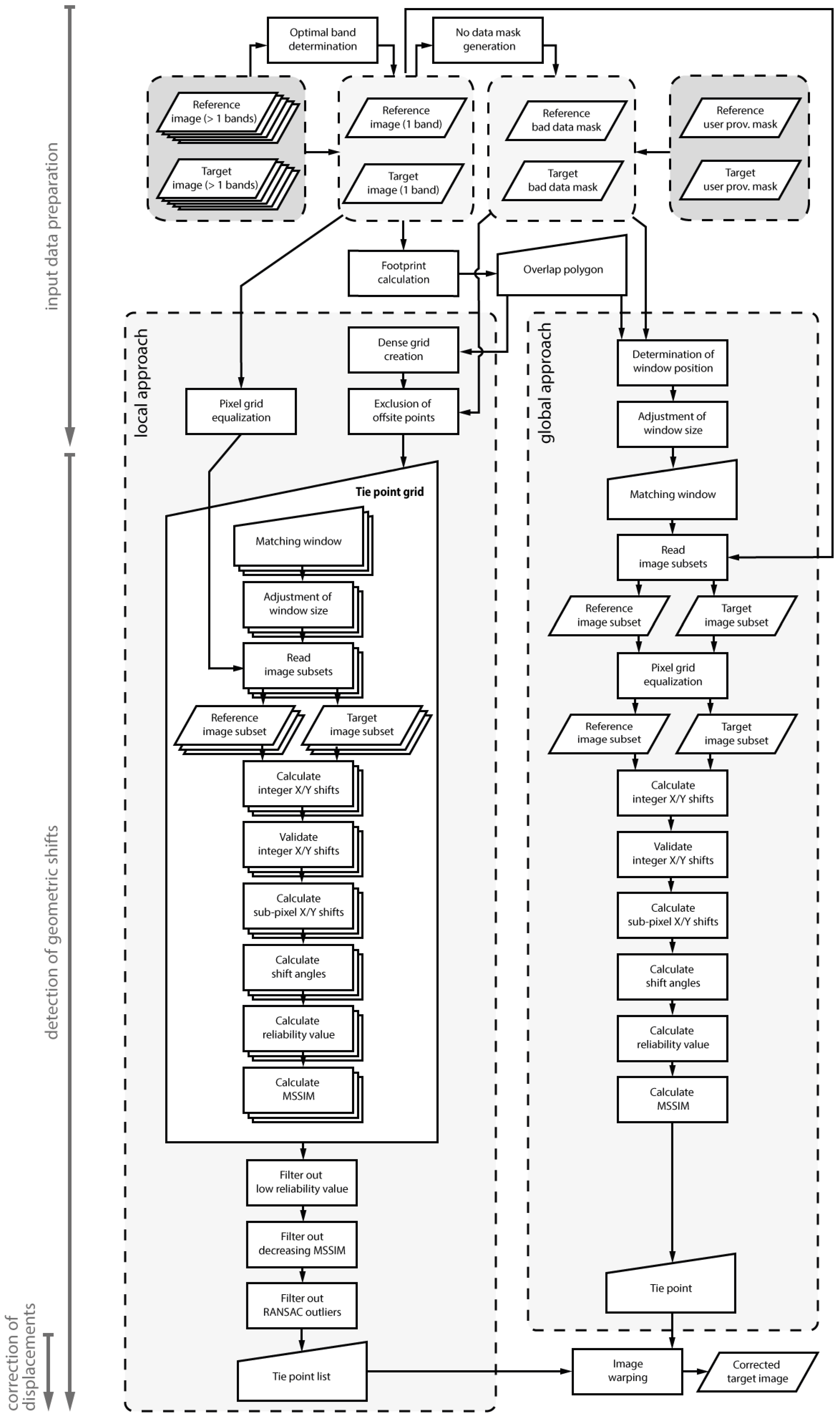
2.1. Algorithm Overview
- Input data preparation (Section 2.2) including: (1) automatic selection of the spectral bands from target and reference image to be used for co-registration; (2) no-data mask generation and combination with user-provided masks (e.g., containing clouds and cloud shadows) to separate bad-data masks for reference and target image; (3) calculation of the respective footprint polygons and corresponding overlap area; (4) pixel coordinate grid equalization; and (5) adjustment of matching window positions and sizes
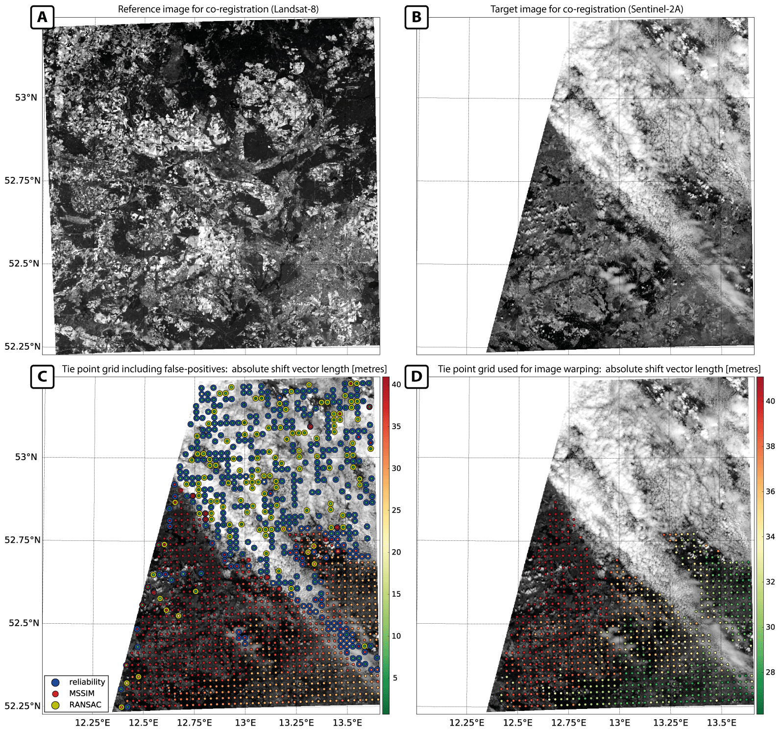
- Detection of geometric shifts (Section 2.3), either in a moving-window manner for each point of a dense grid (local co-registration approach) or for only a single coordinate position (global co-registration approach), including validation
- Correction of displacements (Section 2.4), by warping the target image under the use of a list of tie points (local co-registration approach) or a single X/Y shift vector (global co-registration approach)
2.2. Input Data Preparation
2.2.1. Obligatory and Optional Input Data and Parameters
2.2.2. Determination of Optimal Spectral Bands Used for Matching
2.2.3. Calculation of Overlap Area between the Input Datasets
2.2.4. Pixel Grid Equalization
2.2.5. Adjustment of Matching Window Positions and Sizes
2.3. Detection of Geometric Shifts
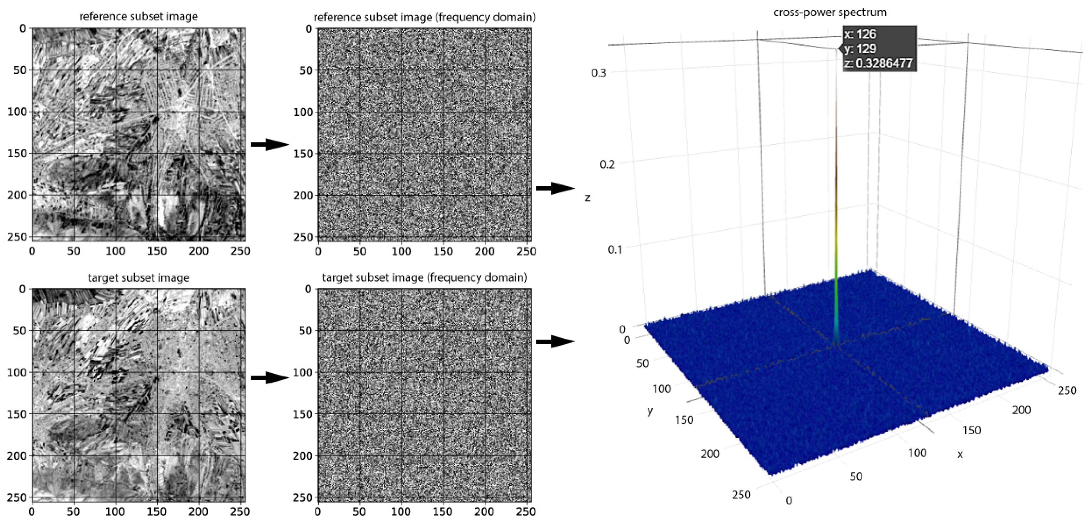
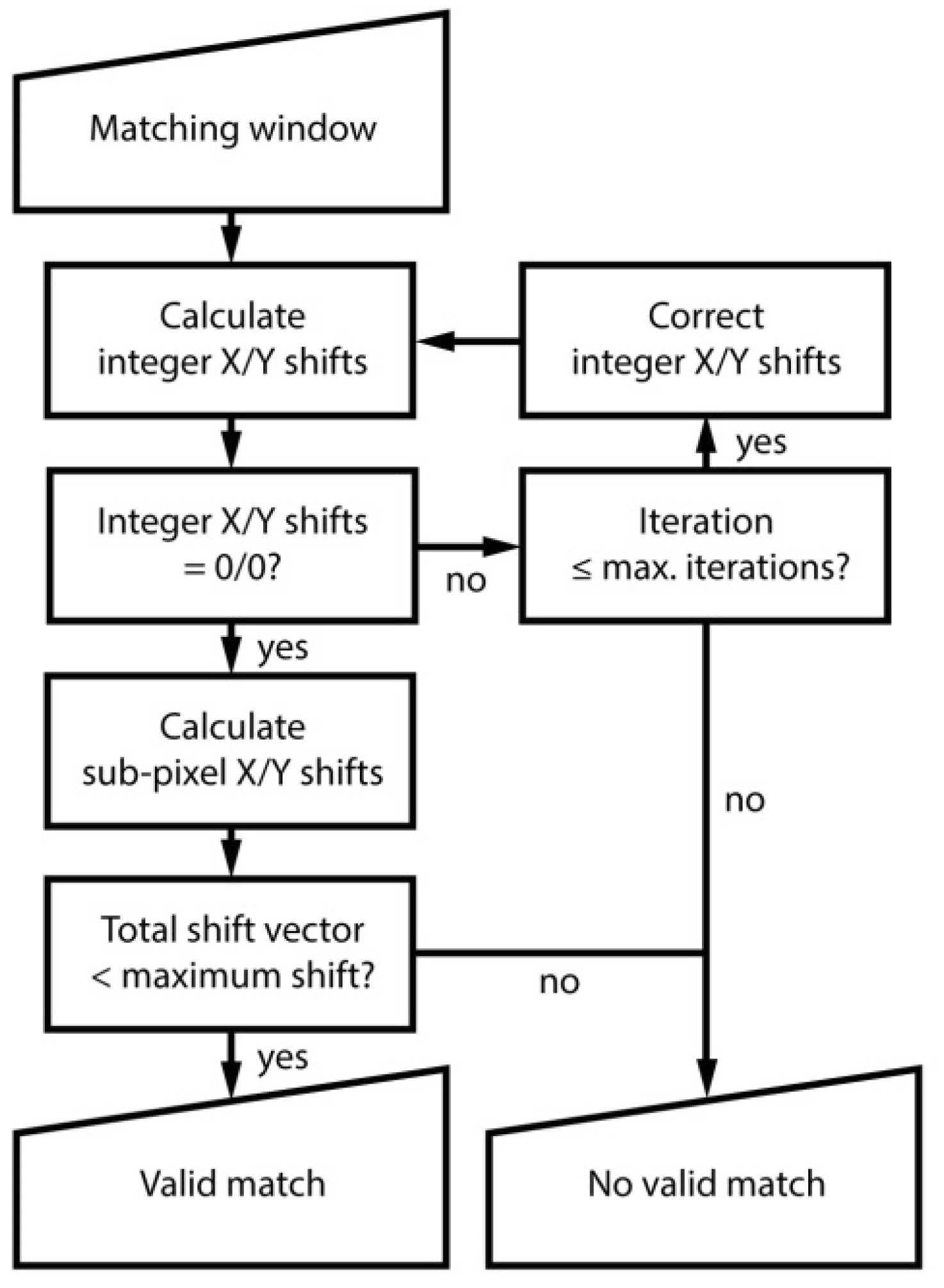
2.3.1. Calculation of Geometric Shifts within the Matching Window
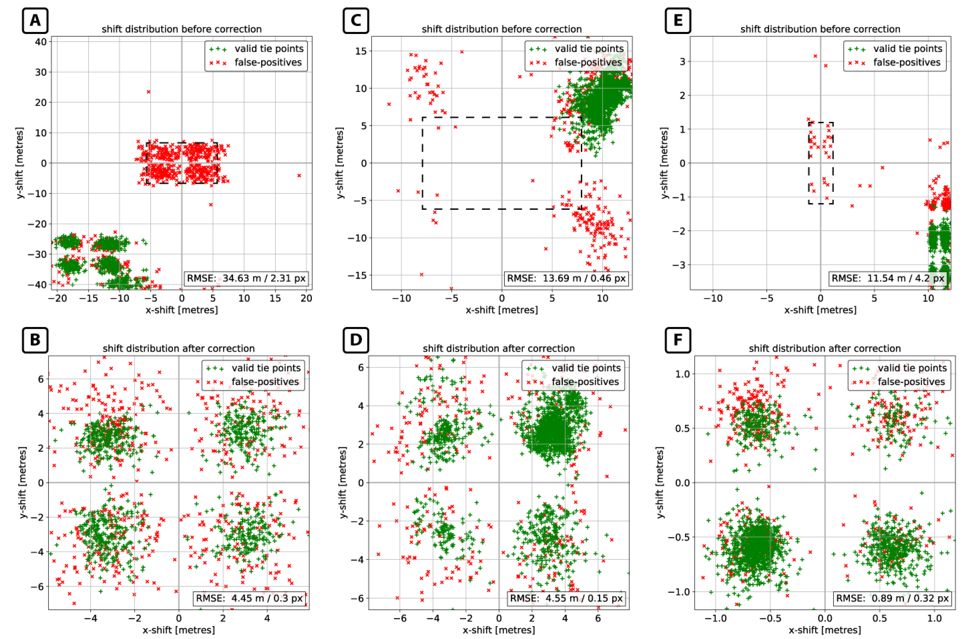
2.3.2. Validation of Calculated Spatial Shifts
2.4. Correction of Displacements
3. Sample Data
4. Results and Discussion
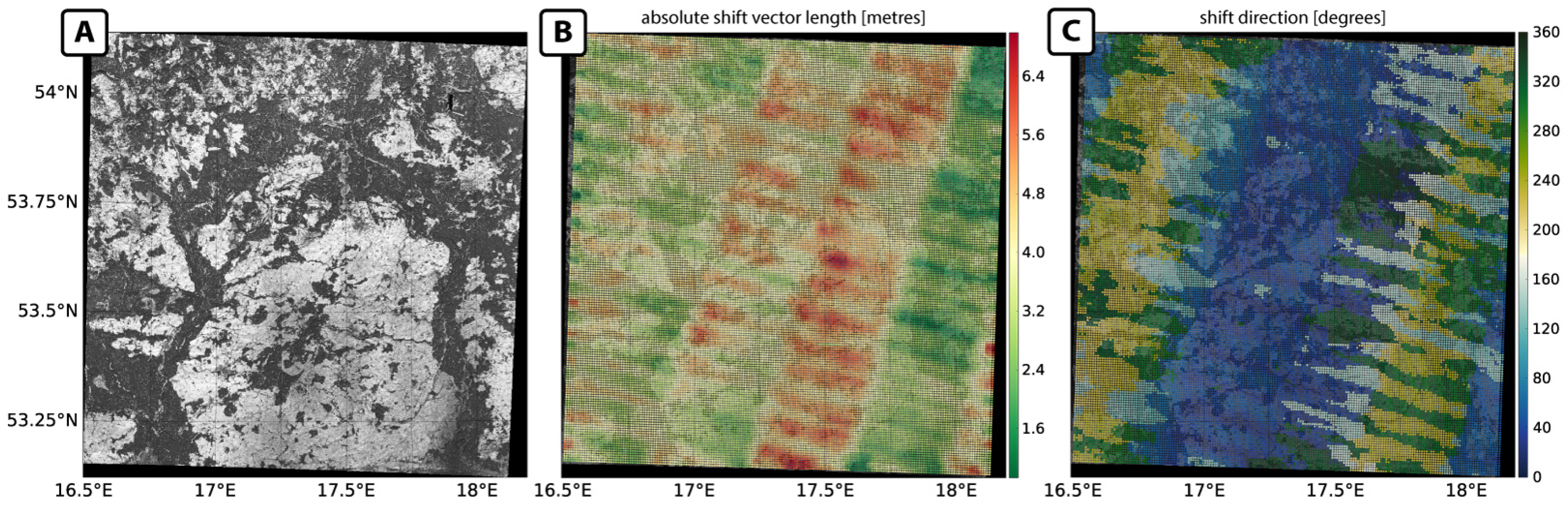
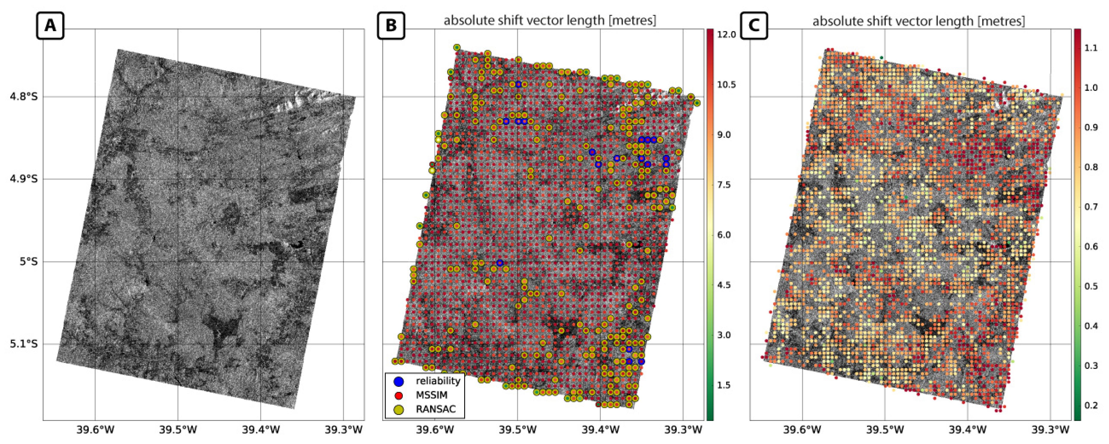
4.1. Inter-Sensoral Use Cases
4.2. Intra-Sensoral Use Cases
5. Algorithm Performance
5.1. Co-Registration Performance
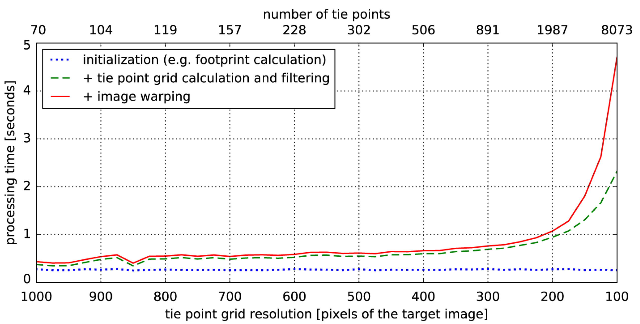
5.2. Computational Efficiency
5.3. Performance Comparison to State of the Art Co-Registration Workflows
6. Conclusions
Acknowledgments
Author Contributions
Conflicts of Interest
References
- Townshend, J.R.G.; Justice, C.O.; Gurney, C.; McManus, J. The Impact of Misregistration on Change Detection. IEEE Trans. Geosci. Remote Sens. 1992, 30, 1054–1060. [Google Scholar] [CrossRef]
- Dai, X.; Khorram, S. The effects of image misregistration on the accuracy of remotely sensed change detection. IEEE Trans. Geosci. Remote Sens. 1998, 36, 1566–1577. [Google Scholar]
- Liang, J.; Liu, X.; Huang, K.; Li, X.; Wang, D.; Wang, X. Automatic Registration of Multisensor Images Using an Integrated Spatial and Mutual Information ( SMI ) Metric. IEEE Trans. Geosci. Remote Sens. 2014, 52, 603–615. [Google Scholar] [CrossRef]
- Sundaresan, A.; Varshney, P.K.; Arora, M.K. Robustness of Change Detection Algorithms in the Presence of Registration Errors. Photogramm. Eng. Remote Sens. 2007, 73, 375–383. [Google Scholar] [CrossRef]
- Behling, R.; Roessner, S.; Segl, K.; Kleinschmit, B.; Kaufmann, H. Robust Automated Image Co-Registration of Optical Multi-Sensor Time Series Data: Database Generation for Multi-Temporal Landslide Detection. Remote Sens. 2014, 6, 2572–2600. [Google Scholar] [CrossRef]
- Swain, P.H.; Vanderbilt, V.C.; Jobusch, C.D. A quantitative applications-oriented evaluation of thematic mapper design specifications. IEEE Trans. Geosci. Remote Sens. 1982, 75, 370–377. [Google Scholar] [CrossRef]
- Le Moigne, J.; Netanyahu, N.S.; Eastman, R.D. Image Registration for Remote Sensing, 1st ed.; Cambridge University Press: Cambridge, UK, 2011. [Google Scholar]
- Dalmiya, C.P.; Dharun, V.S. A Survey of Registration Techniques in Remote Sensing Images. Indian J. Sci. Technol. 2015, 8, 1–7. [Google Scholar] [CrossRef]
- Zitová, B.; Flusser, J. Image registration methods: A survey. Image Vis. Comput. 2003, 21, 977–1000. [Google Scholar] [CrossRef]
- Chen, H.; Arora, M.K.; Varshney, P.K. Mutual information based image registration for remote sensing data. Electr. Eng. Comput. Sci. 2003, 24, 3701–3706. [Google Scholar] [CrossRef]
- Long, T.; Jiao, W.; He, G.; Zhang, Z. A fast and reliable matching method for automated georeferencing of remotely-sensed imagery. Remote Sens. 2016, 8, 56. [Google Scholar] [CrossRef]
- Dawn, S.; Vikas, S.; Sharma, B. Remote Sensing Image Registration Techniques: A Survey. In Image and Signal Processing. ICISP 2010. Lecture Notes in Computer Science; Elmoataz, A., Lezoray, O., Nouboud, F., Mammass, D., Meunier, J., Eds.; Springer: Berlin/Heidelberg, Germany, 2010; Volume 6134, pp. 103–112. [Google Scholar]
- Brown, L.G. A survey of image registration techniques. ACM Comput. Surv. 1992, 24, 325–376. [Google Scholar] [CrossRef]
- Gianinetto, M. Automatic Co-Registration of Satellite Time Series. Photogramm. Rec. 2012, 27, 462–470. [Google Scholar] [CrossRef]
- Wong, A.; Clausi, D.A. ARRSI: Automatic registration of remote-sensing images. IEEE Trans. Geosci. Remote Sens. 2007, 45, 1483–1492. [Google Scholar] [CrossRef]
- Leprince, S.; Barbot, S.; Ayoub, F.; Avouac, J.P. Automatic and Precise Orthorectification and Coregistration and Subpixel Correlation of Satellite Images, Application to Ground Deformation Measurements. IEEE J. Geosci. Rem. Sens. 2007, 45, 1529–1558. [Google Scholar] [CrossRef]
- Gao, F.; Masek, J.G.; Wolfe, R.E. Automated registration and orthorectification package for Landsat and Landsat-like data processing. J. Appl. Remote Sens. 2009, 3, 33515. [Google Scholar]
- Yan, L.; Roy, D.; Zhang, H.; Li, J.; Huang, H. An Automated Approach for Sub-Pixel Registration of Landsat-8 Operational Land Imager (OLI) and Sentinel-2 Multi Spectral Instrument (MSI) Imagery. Remote Sens. 2016, 8, 520. [Google Scholar] [CrossRef]
- Foroosh, H.; Zerubia, J.B.; Berthod, M. Extension of phase correlation to subpixel registration. IEEE Trans. Image Process. 2002, 11, 188–199. [Google Scholar] [CrossRef] [PubMed]
- Chen, Q.; Defrise, M.; Deconinck, F. Symmetric Phase-Only Matched Filtering of Fourier-Mellin Transforms for Image Registration and Recognition. IEEE Trans. Pattern Anal. Mach. Intell. 1994, 16, 1156–1168. [Google Scholar] [CrossRef]
- Heid, T.; Kääb, A. Evaluation of existing image matching methods for deriving glacier surface displacements globally from optical satellite imagery. Remote Sens. Environ. 2012, 118, 339–355. [Google Scholar] [CrossRef]
- Rogass, C.; Segl, K.; Kuester, T.; Kaufmann, H. Performance of correlation approaches for the evaluation of spatial distortion reductions. Remote Sens. Lett. 2013, 4, 1214–1223. [Google Scholar] [CrossRef]
- Joglekar, J.; Gedam, S.S. Area Based Image Matching Methods—A Survey. Int. J. Emerg. Technol. Adv. Eng. 2012, 2, 130–136. [Google Scholar]
- Tong, X.; Ye, Z.; Xu, Y.; Liu, S.; Li, L.; Xie, H.; Li, T. A Novel Subpixel Phase Correlation Method Using Singular Value Decomposition and Unified Random Sample Consensus. IEEE Trans. Geosci. Remote Sens. 2015, 53, 4143–4156. [Google Scholar] [CrossRef]
- Storey, J.; Roy, D.P.; Masek, J.; Gascon, F.; Dwyer, J.; Choate, M. A note on the temporary misregistration of Landsat-8 Operational Land Imager (OLI) and Sentinel-2 Multi Spectral Instrument (MSI) imagery. Remote Sens. Environ. 2016, 186, 121–122. [Google Scholar] [CrossRef]
- Yoon, Y.T.; Eineder, M.; Yague-Martinez, N.; Montenbruck, O. TerraSAR-X precise trajectory estimation and quality assessment. IEEE Trans. Geosci. Remote Sens. 2009, 47, 1859–1868. [Google Scholar] [CrossRef]
- Young, N.E.; Anderson, R.S.; Chignell, S.M.; Vorster, A.G.; Lawrence, R.; Evangelista, P.H. A survival guide to Landsat preprocessing. Ecology 2017, 98, 920–932. [Google Scholar] [CrossRef] [PubMed]
- Bracewell, R.N. The Fourier Transform and Its Applications; McGraw-Hill: New York, NY, USA, 1965. [Google Scholar]
- Open Source Geospatial Foundation. GDAL Raster Formats. Available online: http://www.gdal.org/formats_list.html (accessed on 19 April 2017).
- Luan, X.; Yu, F.; Zhou, H.; Li, X.; Song, D.; Wu, B. Illumination-robust area-based stereo matching with improved census transform. In Proceedings of the 2012 International Conference on Measurement, Information and Control (MIC), Harbin, China, 18–20 May 2012; Volume 1, pp. 194–197. [Google Scholar]
- Frigo, M.; Johnson, S.G. The design and implementation of FFTW3. Proc. IEEE 2005, 93, 216–231. [Google Scholar] [CrossRef]
- Frigo, M.; Johnson, S. The Fastest Fourier Transform in the West. Technical Report MIT-LCS-TR-728; MIT Lab for Computer Science: Cambridge, MA, USA, 1997. [Google Scholar]
- Kuglin, C.D.; Hines, D.C. The phase correlation image alignment method. In Proceedings of the IEEE Conference on Cybernetics and Society, Banff, AB, Canada, 1–4 October 1975; pp. 163–165. [Google Scholar]
- Keller, Y.; Averbuch, A.; Israeli, M. Pseudo-polar based estimation of large translations rotations and scalings in images. IEEE Trans. Image Process. 2005, 14, 12–22. [Google Scholar] [CrossRef] [PubMed]
- Wang, Z.; Bovik, A.C.; Sheikh, H.R.; Simoncelli, E.P. Image quality assessment: From error visibility to structural similarity. IEEE Trans. Image Process. 2004, 13, 600–612. [Google Scholar] [CrossRef] [PubMed]
- Avanaki, A.N. Exact global histogram specification optimized for structural similarity. Opt. Rev. 2009, 16, 613–621. [Google Scholar] [CrossRef]
- Fischler, M.A.; Bolles, R.C. Random Sample Consensus: A Paradigm for Model Fitting with Applicatlons to Image Analysis and Automated Cartography. Commun. ACM 1981, 24, 381–395. [Google Scholar] [CrossRef]
- Hast, A.; Nysjö, J.; Marchetti, A. Optimal RANSAC—Towards a repeatable algorithm for finding the optimal set. J. WSCG 2013, 21, 21–30. [Google Scholar]
- Toldo, R.; Fusiello, A. Automatic estimation of the inlier threshold in robust multiple structures fitting. In Image Analysis and Processing—ICIAP 2009. ICIAP 2009. Lecture Notes in Computer Science; Foggia, P., Sansone, C., Vento, M., Eds.; Springer: Berlin/Heidelberg, Germany, 2009; Volume 5716, pp. 123–131. [Google Scholar]
- Subbarao, R.; Meer, P. Beyond RANSAC: User independent robust regression. In Proceedings of the IEEE Computer Society Conference on Computer Vision and Pattern Recognition, New York, NY, UAS, USA 17–23 July 2006; Volume 2006. [Google Scholar]
- Earthstar Geographics LCC. TerraColor® Global Landsat Satellite Images of Earth. Available online: http://www.terracolor.net/index.html (accessed on 19 April 2017).
- Chander, G.; Haque, M.O.O.; Sampath, A.; Brunn, A.; Trosset, G.; Hoffmann, D.; Roloff, S.; Thiele, M.; Anderson, C. Radiometric and geometric assessment of data from the RapidEye constellation of satellites. Int. J. Remote Sens. 2013, 34, 37–41. [Google Scholar] [CrossRef]
- Clerc, S. Sentinel-2 Data Quality Report Issue 1 (November 2015). Ref. S2-PDGS-MPC-DQR, European Space Agency (ESA). Available online: https://earth.esa.int/documents/247904/685211/Sentinel-2+Data+Quality+Report+Issue+01+%28November+2015%29/74295984-60d0-479e-b6ea-f04e25a84f5a?version=1.2 (accessed on 22 April 2017).
- Gascon, F.; Thépaut, O.; Jung, M.; Francesconi, B.; Louis, J.; Lonjou, V.; Lafrance, B.; Massera, S.; Gaudel-Vacaresse, A.; Languille, F.; et al. Copernicus Sentinel-2 Calibration and Products Validation Status. Remote Sens. 2017, 9, 584. [Google Scholar] [CrossRef]
- Zhang, S.; Foerster, S.; Medeiros, P.; Waske, B. Monitoring water extent in macrophyte covered reservoirs in NE Brazil using TerraSAR-X time series data. (submitted).
- Nobach, H.; Honkanen, M. Two-dimensional Gaussian regression for sub-pixel displacement estimation in particle image velocimetry or particle position estimation in particle tracking velocimetry. Exp. Fluids 2005, 38, 511–515. [Google Scholar] [CrossRef]
- Averbuch, A.; Keller, Y. FFT based image registration. In Proceedings of the IEEE International Conference on Acoustics Speech and Signal Processing, Orlando, FL, USA, 13–17 May 2002; pp. IV-3608–IV-3611. [Google Scholar]
- Helmholtz-Centre Potsdam—GFZ German Research Centre for Geosciences. GFZ Time Series System for Sentinel-2. Available online: http://www.gfz-potsdam.de/gts2 (accessed on 19 April 2017).


| Name | Reference/Target Image (R/T) | Sensor | Acquisition Date | Spatial Resolution (m) | Image Dimensions (Rows, Columns) | Processing Level |
|---|---|---|---|---|---|---|
| INTER1 | R | Landsat-8, band 2 | <multiple> | 15 | 7320, 7320 | 1T |
| T | Sentinel-2A, band 3 | 29 May 2016 | 10 | 10,980, 10,980 | 1C | |
| INTER2 | R | Landsat-8, band 5 | 1 June 2013 | 30 | 7541, 7721 | 1T |
| T | RapidEye, band 5 | 23 April 2013 | 5 | 5000, 5000 | 3A | |
| INTRA1 | R | Sentinel-2A, band 7 | 11 January 2017 | 20 | 5490, 5490 | 1C |
| T | Sentinel-2A, band 8A | 11 January 2017 | 20 | 5490, 5490 | 1C | |
| INTRA2 | R | TerraSAR-X, X-band | 10 February 2014 | 2.75 | 19,090, 15,636 | EEC |
| T | TerraSAR-X, X-band | 1 January 2015 | 2.75 | 19,090, 15,636 | EEC |
© 2017 by the authors. Licensee MDPI, Basel, Switzerland. This article is an open access article distributed under the terms and conditions of the Creative Commons Attribution (CC BY) license (http://creativecommons.org/licenses/by/4.0/).
Share and Cite
Scheffler, D.; Hollstein, A.; Diedrich, H.; Segl, K.; Hostert, P. AROSICS: An Automated and Robust Open-Source Image Co-Registration Software for Multi-Sensor Satellite Data. Remote Sens. 2017, 9, 676. https://doi.org/10.3390/rs9070676
Scheffler D, Hollstein A, Diedrich H, Segl K, Hostert P. AROSICS: An Automated and Robust Open-Source Image Co-Registration Software for Multi-Sensor Satellite Data. Remote Sensing. 2017; 9(7):676. https://doi.org/10.3390/rs9070676
Chicago/Turabian StyleScheffler, Daniel, André Hollstein, Hannes Diedrich, Karl Segl, and Patrick Hostert. 2017. "AROSICS: An Automated and Robust Open-Source Image Co-Registration Software for Multi-Sensor Satellite Data" Remote Sensing 9, no. 7: 676. https://doi.org/10.3390/rs9070676
APA StyleScheffler, D., Hollstein, A., Diedrich, H., Segl, K., & Hostert, P. (2017). AROSICS: An Automated and Robust Open-Source Image Co-Registration Software for Multi-Sensor Satellite Data. Remote Sensing, 9(7), 676. https://doi.org/10.3390/rs9070676