Article

Spatiotemporal Variation in Particulate Organic Carbon Based on Long-Term MODIS Observations in Taihu Lake, China

1
School of geography science, Nanjing Normal University, Nanjing 210023, China
2
State Key Laboratory of Lake Science and Environment, Nanjing Institute of Geography and Limnology, Chinese Academy of Sciences, Nanjing 210023, China
3
State Key Laboratory of Resources and Environmental Information System, Institute of Geographic Sciences and Natural Resources Research, Chinese Academy of Sciences, Beijing 100101, China
4
Guangdong Institute of Geography, Guangdong academy of sciences, Guangzhou 510070, China
5
Key Laboratory of Virtual Geographic Environment (Nanjing Normal University), Ministry of Education, Nanjing 210023, China
6
Jiangsu Center for Collaborative Innovation in Geographical Information Resource Development and Application, Nanjing Normal University, Nanjing 210023, China
*
Author to whom correspondence should be addressed.
Remote Sens. 2017, 9(6), 624; https://doi.org/10.3390/rs9060624
Submission received: 8 May 2017 / Revised: 26 May 2017 / Accepted: 15 June 2017 / Published: 17 June 2017
(This article belongs to the Special Issue Remote Sensing of Water Quality)

Abstract

:
In situ measured values of particulate organic carbon (POC) in Taihu Lake and remote sensing reflectance observed by three satellite courses from 2014 to 2015 were used to develop an near infrared-red (NIR-Red) empirical algorithm of POC for the Moderate Resolution Imaging Spectroradiometer (MODIS-Aqua) satellite image. The performance of the POC algorithm is highly consistent with the in situ measured POC, with root mean square error percentage (RMSPs) of 38.9% and 31.5% for two independent validations, respectively. The MODIS-derived POC also shows an acceptable result, with RMSPs of 53.6% and 61.0% for two periods of match-up data. POC from 2005 to 2007 is much higher than it is from 2002 to 2004 and 2008 to 2013, due to a large area of algal bloom. Riverine flux is an important source of POC in Taihu Lake, especially in the lake’s bank and bays. The influence of a terrigenous source of POC can reach the center lake during periods of heavy precipitation. Sediment resuspension is also a source of POC in the lake due to the area’s high dynamic ratio (25.4) and wind speed. The source of POC in an inland shallow lake is particularly complex, and additional research on POC is needed to more clearly reveal its variation in inland water.

Graphical Abstract

1. Introduction

Inland freshwater has an important role in the regional and global carbon cycle despite its small fraction of the earth’s surface relative to the land and ocean [1,2,3,4,5,6,7]. In the global carbon cycle, inland freshwater is not only a pivotal point for carbon transport between terrestrial and marine (about 0.9 Pg C y−1) locations, but it also serves to bury terrestrially derived carbon (about 0.98 Pg C y−1). This buried carbon will be emitted to the atmosphere as CO2 (0.75 Pg C y−1) during the mineralization process of carbon and finally stored in the sediment (0.23 Pg C y−1) [4,8]. Particulate organic carbon (POC) in inland waters is an important carbon pool that has a clear effect on dissolved organic and inorganic carbon due to the degradation and mineralization [2,9,10]. Little change in the POC of inland water will indicate that there are substantial changes in related carbon fluxes, even though POC represents only a small portion of the total carbon reservoir on a global scale [11,12,13,14]. A detailed understanding of the distribution and long-term patterns of POC in inland water is therefore important to understanding the carbon cycle in inland water and its effect on the global carbon cycle [15,16,17,18].
Large POC-retrieval algorithms for application in remote sensing have been developed because they have the advantage of providing synchronous and timely observations over a large area [12,14,19,20,21,22,23,24,25,26]. Some of these POC algorithms, which are based on the relationships between POC and optical properties (backscattering coefficient, beam attenuation and diffuse attenuation coefficient), performed very well in open ocean waters [19,20,22,27,28,29,30]. An empirical algorithm based on the blue and green bands was also used to estimate POC and showed high accuracy in oceans [12,25,31]. However, these POC algorithms fail in inland waters due to the much more complex optical properties [32]. This significantly limits the gathering of large-scale and long-term properties of POC distribution over time in inland water bodies. Several new POC retrieval algorithms focusing on inland turbid and eutrophic water were developed and applied to remote sensing satellite data [32,33,34]. Most of these POC retrieval algorithms for inland water are based on the near infrared and red bands due to the low impact of tripton and colored dissolved organic matter [35]. Nevertheless, long-term observation of POC in inland water is still scarce due to the limitations of the validated atmospheric correction method and POC algorithms for specific satellite images (such as Moderate-resolution Imaging Spectroradiometer (MODIS)) [33]. It is thus difficult to evaluate the historical levels and changing trends of POC in inland water. The validated POC algorithm and atmospheric correction method for satellite images, which have a long-term observation dataset, are useful for assessing of the carbon status of inland waters from remote sensing [32,33,34]. The amount of POC data for inland water is still insufficient for the development of validated POC algorithms, although several studies have described the large-scale distributions and short-term variations of POC in the inland water [32,33,36]. Thus, much is still not well understood about POC in inland water, and field measurements and POC-retrieval algorithms are needed to capture its changing trends.
The storage of POC in Taihu Lake is highly variable because of the strong influence of terrestrial carbon input, sedimentary releases from sediment resuspension and local biological products. This study develops an NIR-Red band ratio empirical algorithm of POC, based on the in situ POC measurement data and remote sensing reflectance (Rrs) in Taihu Lake. This empirical algorithm was then applied to satellite data from MODIS to obtain the long-term distribution of POC. The primary objective is to reveal long-term spatial and temporal variation in the POC in Taihu Lake during the period 2002–2014, and to evaluate the factors influencing this variation.

2. Materials and Methods

2.1. Study Area and Sampling

Taihu Lake is a eutrophic lake with the third largest lake area (2338 km2) in China; the lake is located downstream of the Yangtze River. The lake faces crucial issues of eutrophication and the consequent algal bloom [37,38]. The concentration of Dissolved Organic Carbon (DOC) in the lake can reach 7.21 mg/L with mean value of 4.51 ± 0.89 mg/L (mean value ± standard deviation) and the concentration of POC can reach 18.07 mg/L with mean value of 5.45 ± 6.28 mg/L from in situ measurements [38]. The optical-property and water-constituent measurements were made during five cruises over a period from 2014 to 2015 (namely, 5 August 2014, 24 October 2014, 21 May 2015, 10 June 2015 and 15 July 2015). The coverage of sampling stations was evenly distributed across the entire lake (Figure 1). The total number of sampling stations with POC data was 197 (this study dataset), and 143 samples were randomly selected to calibrate the POC-retrieval algorithm; the remaining 54 samples (validation data) were used to validate the POC algorithm. The match-up points for the validation of atmospheric correction were 129 during 2006 to 2014 from Huang [39].

2.2. Optical Property Measurements

Remote sensing reflectance (Rrs) was obtained by measuring the radiance of water, sky and gray panels. The detailed steps and calculation method follows methods described by Huang [39] and Lee [40]. The absorption coefficient of pigment phytoplankton (aph), no-pigment matter (aNAP) and chromophoric dissolved organic matter (aCDOM) were measured using a quantitative membrane filter technique with spectrophotometer [41].

2.3. Water Constituent Measurement

Water samples were collected from surface water (30 cm) and stored in Niskin bottles in ice. The water was filtered through pre-combusted (450 °C for 4 h) Whatman glass fiber filters (GF/F) under a low vacuum. A filter with suspended particles was dried at 55 °C for 8 hours, and then treated with 0.01 mol/L HCl to remove inorganic carbon. After acidification treatment, the filter was dried again and weighed. POC concentration (mg/L) was determined by the combustion of the filter in a carbon elemental analyzer (TOC-L-SSM-5000A, Shimadzu Corporation) [42].
The concentration of chlorophyll-a (Chl-a) was measured by a spectrophotometric method with hot alcohol (90%) [41]. The concentration of phycocyanin (PC) was determined by spectrofluorimetry [43]. The concentrations of total suspended particulate matter (SPM), organic suspended matter (OSM), and inorganic suspended matter (ISM) were detected following the gravimetric method [41].

2.4. MODIS Data Processing

Medium-resolution satellite data (with 250 m spatial resolution) from MODIS Aqua Level 0 images from June 2002 to 2014, with no or minimal cloud cover, were chosen and downloaded from the US NASA Goddard Space Flight Center (GSFC, http://oceancolor.gsfc.nasa.gov). SeaDAS 6.4 was used to produce the radiometric and geometric correction of acquired MODIS Aqua Level 0 data. The corresponding MODIS cloud mask products (MOD35) were used to perform the cloud masking.
Satellite angle information (solar zenith angle, solar azimuth angle, satellite zenith angle, and satellite azimuth angle), ozone, and water vapor content from SeaDAS 6.4 were used as input parameters in the atmospheric correction. The atmospheric correction method was based on the hypothesis that water reflectance at near-infrared band is zero [44] and may generate large errors in inland turbid water due to the high reflectance at near-infrared wavelength [45,46]. An improved land target-based atmospheric correction method [47,48] was selected to derive the reflectance from the MODIS-Aqua data over Taihu Lake. This method involves three simple steps: first, the selection of dense dark vegetation (DDV) pixels from lakeshore and island areas; second, the retrieval of the aerosol optical thickness at 550 nm (AOT550) for the selected DDV pixels; and third, the retrieval of the remote sensing reflectance over water. The DDV pixels were selected from 5-km buffer along the lakeshore and island of Taihu Lake. The mixed pixels were eliminated via a checking process with 3 × 3 uniformity windows. The DDV pixel was reserved only when all nine pixels (3 × 3 windows) were preliminary DDV pixels. DDV pixels with NDVI were chosen to derive AOT550. AOT550 for each pixel in Taihu Lake was from spatial interpolation of retrieved AOT550 for DDV pixels. For detailed process steps can refer to Liu [48].

2.5. Statistical Analysis and Accuracy

Data were analyzed to calculate the spatial and temporal average value of POC for different lake segments and times (monthly), and the temporal average value of POC (seasonal and annual) for the whole lake. We compiled an Interactive Data Language (IDL) program to complete the statistical analysis and map the box figures. The accuracy of the retrieval algorithm was evaluated by root mean square error percentage (RMSP), which expresses the normalized difference between measured and retrieved value to measured value. It can be calculated using Equation (1).
R M S P = i = 1 n [ ( C POC - r C POC - m ) / C POC - m ] 2 n
where CPOC-r and CPOC-m are the retrieved and measured concentrations of POC, respectively.

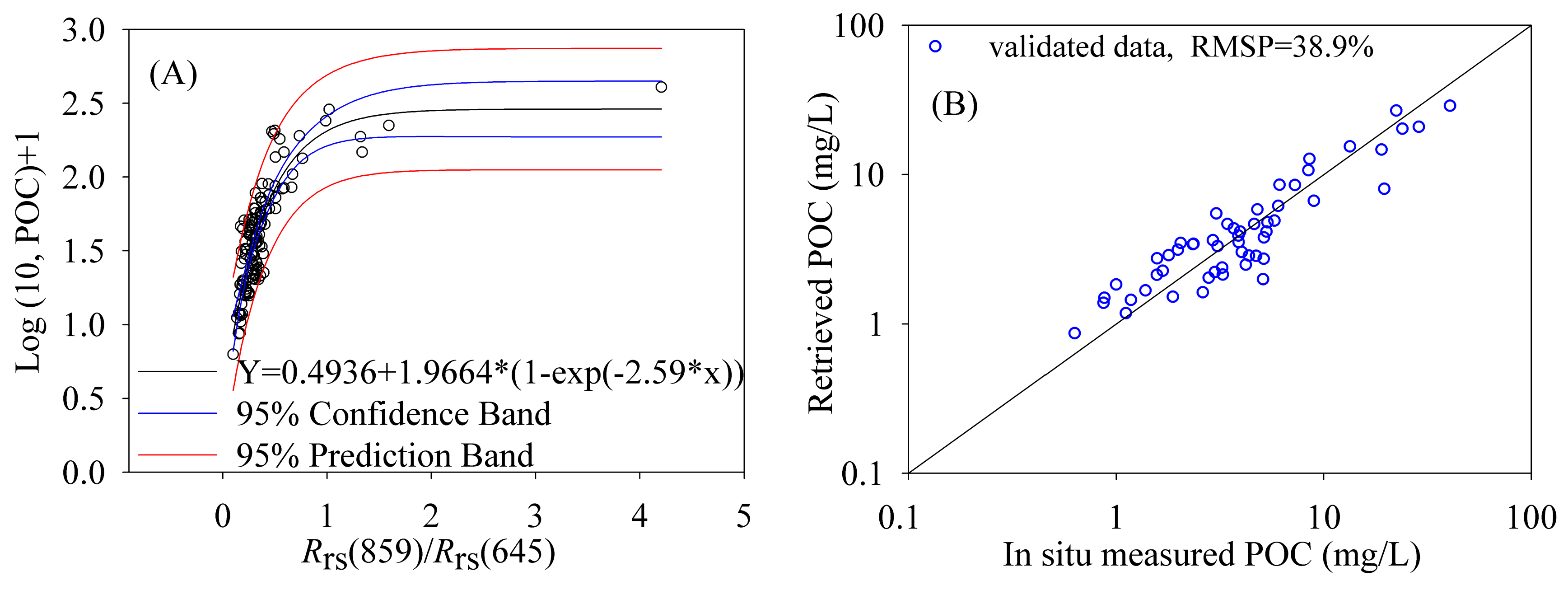
3. Calibration and Validation of NIR-Red Empirical Algorithm of POC

Our POC-retrieval algorithm relies on the empirical relationship between surface POC concentration and remote sensing reflectance. The reflectance at a specific wavelength was determined using an optimized iterative algorithm between POC and band ratio of remote sensing reflectance [39,49]. The optimal spectral bands (λ2 and λ1) were determined by the iteration of the MODIS band’s setting. Finally, the NIR-Red band ratio (Rrs (859)/Rrs (645)) empirical algorithm for POC was confirmed. The calibration result shows that the exponential growth function fits the co-variation between POC and Rrs (859)/Rrs (645) well (Figure 2A). The NIR-Red band ratio in the empirical POC algorithm is very similar to the current algorithm of chlorophyll-a concentration in inland water (or turbid case II water) [39,49,50,51,52]. This also occurs in the ocean, where the blue-green band ratio in the POC algorithm is very similar to the current algorithm of ocean chlorophyll-a concentration [53]. This could be caused by any number of POC-containing particles, which include both pigmented phytoplankton and organic detritus, and have higher absorption in the blue spectral region. However, in inland water, the POC-containing particles, not just particles of phytoplankton, but also total suspended particulate matter, have specific fluorescence and scattering properties in the red and near-infrared spectral region [52,54,55]. All calibration data in the POC retrieval algorithm were in the 95% confidence line of the linear regression, and the best regression equation in the 95% prediction line can be expressed as Equation (2):
y = 10 f POC ( MODIS ) 1
f POC ( MODIS ) = 0.4936 + 1.9664 * ( 1 exp ( 2.59 * R rs ( 859 ) R rs ( 645 ) ) )
N = 143, R2 = 0.73, p < 0.0001
The validation result for validation data indicates that the POC-retrieval algorithm can measure POC successfully with relatively high accuracy. The RMSP of validation data is 38.9% (Figure 2B). However, this model will underestimate extremely high POC (>30 mg/L), and the underestimated error will increase with high POC.
To further verify the performance of the POC algorithm to MODIS satellite data, the match-up points were used to validate the atmospheric correction (match-up points for the Rrs) and POC-retrieval results (match-up points for the Rrs and POC). The match-up MODIS satellite image was selected with the condition that the time interval for matching MODIS and in situ Rrs was less than three hours (similar to Cédric et al. [56]). The match-up pixel is consistent with the coordinates of the sampling site. The performance of this improved land target-based atmospheric correction method is acceptable for turbid water or eutrophic water, aside from some blue and green bands (Figure 3A). The atmospheric correction results indicate that the accuracy of Rrs (645) retrieved by MODIS is much better than that of Rrs (859). The RMSP of Rrs (645) and Rrs (859) are 22.6% and 40.2%, respectively. The RMSP of band ratio of Rrs (645) and Rrs (859) is 29.6%. The accuracy of MODIS-derived Rrs (859)/Rrs (645) is better than that of Rrs (859), but worse than that of Rrs (645) (Figure 3B). The validation of match-up points for the POC-retrieval algorithm shows that the MODIS-derived POC is highly consistent with the in situ measured data. The RMSP between MODIS-derived POC and POC measured on 5 August 2014 and 24 October 2014 is 53.6% and 61.0%, respectively (Figure 3C). The validation of the atmospheric correction and POC-retrieval algorithm shows the applicability of the algorithm to MODIS satellite data.

4. Results

4.1. Temporal and Spatial Variations of POC

4.1.1. Annual Scale

MODIS Rrs data were used to extract the long-term temporal and spatial distribution of POC in Taihu Lake via a POC-retrieval algorithm (Equation (2)). The annual mean value of POC for the entire lake shows that its spatial variation is highly significant. We should note that the POC retrieval result is invalidated in the East Lake and East Bay due to the NIR signal from submerged vegetation [57] and in surrounding land border pixels due to the heavy land border effect. The distribution of POC along the lake’s bank is high, and the lake’s bays, such as Meilaing, Gonghu and Zhushan Bay, show high levels of POC (East Bay should be excluded due to the invalidated POC retrieval result). The POC distribution in the center of the lake is relatively low (Figure 4). This may be explained by the fact that there is a clear influence of POC from terrain on the lake and the phytoplankton is flourishing in the bay and at the shore. The annual variation in the POC distribution shows that the distribution of POC from 2005 to 2007 was relatively more homogeneous than it was from 2002 to 2004 and from 2008 to 2013 (reflected in the difference between the central lake and coastal water). This may be caused by the long period and large area of algal bloom in the lake from 2005 to 2007 [38]. The diffusion and migration of algae from bay and coastal waters obviously increases the POC in the center of the lake.

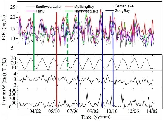
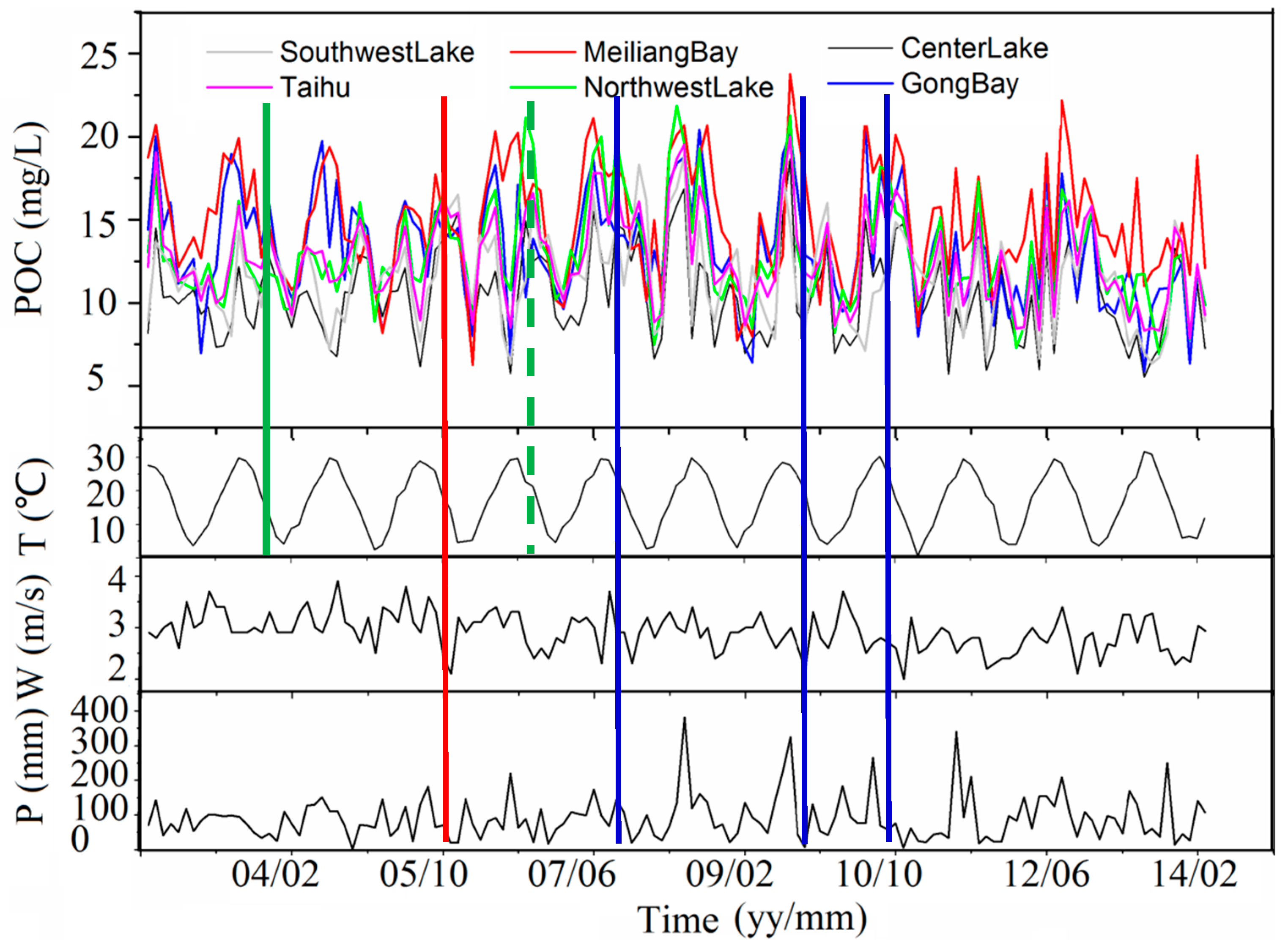
4.1.2. Monthly Scale

The monthly mean POC value for thirteen years was calculated from MODIS-derived daily POC data using the proposed algorithm. The monthly variation in POC shows that the highest POC value appeared in the summer, and the relatively low value occurred in the winter (Figure 5). The high POC level in January is mainly distributed in the southwestern portion of the lake; the level decreased in February, but the relatively low POC in the north of the lake (Meilaing Bay, Gonghu Lake and the northwestern portion of the lake) in January increased significantly. The POC in the north rose dramatically from Match to April, due to the high level of algal growth. This trend of increasing POC in the northern portion of the lake was sustained until August. The POC in the coastal waters increased as well. After August, however, the POC was diffused from north to south in the lake. The POC in the center and the south part of the lake increased significantly. In general, the POC in the lake’s north increased from January to August and then decreased from August to December. The variation trend in the lake’s south almost maintains smoothly high concentration of POC.

4.2. Monthly POC Variation for Each Segment of Taihu Lake

Monthly variation in POC generally increases from January to August, and then decreases from September to December (Figure 6). This trend is probably caused for the most part by two conditions. First, the growth of algae is enhanced with rising temperatures (endogenetic input). Second, the terrestrial input is significantly increased with increasing precipitation (terrestrial input). Both temperature and precipitation have a strong seasonality in Taihu Lake, in which the variation trend is to first increase then decline. However, the asynchronism between temperature and precipitation produced a POC variation trend that is not perfectly consistent with the monthly variation in temperature or precipitation. It is obvious that there is a temporal variation cycle of the high POC concentration (75% red line in Figure 6). Sediment resuspension may be another important factor affecting the inconsistency of POC variation, temperature and precipitation [58].
The different influences of endogenetic and terrestrial input to the POC distribution significantly affected the temporal POC variation in each lake segment. The eastern bay and eastern portion of the lake are extremely limpid with large areas of submerged aquatic plants, and no algal blooms occurred in these areas [57]. The discharge of pollutants in these lake segments is very limited. The POC-retrieval results in the East Bay might be affected by the submerged plants. However, the significant seasonal variation in POC in the east bay allows for a clear view of the growth of aquatic plants (Figure 7 East Bay). This means that the atmospheric-corrected MODIS satellite data have high sensitivity to plant variation (or chlorophyll-a). The POC variation in the eastern portion of the lake is primarily caused by the aquatic plants, and terrestrial input of POC may be important as well.
The monthly POC variation in the lake’s center is not clear (Figure 7 central lake), although several high POC values appeared in summer (August). This indicates that the POC from algae is not the dominant component of POC in the central lake area. This POC might result primarily from sediment resuspension [58]. The other monthly POC variations (Meilaing Bay, Gonghu Bay and the lake’s northwest) are highly significant (Figure 7). It is clear that the dominant component of POC in these areas derives primarily from algae, with the exception of 2013. This is primarily because of the large patches of algal bloom that occur frequently there [38,59], although riverine flux in this area is also significant. The monthly POC variation in the southwestern portion of the lake is not significant. However, different factors influence POC variation in here than in the central lake area. Large areas of algal blooms in the southwest are rare because of the hydrodynamic conditions common in open areas, although it is true that small areas of algal bloom happen frequently there [38]. In addition, this area is in the Tiaoxi Basin, and large quantities of terrestrial POC input were discharged into this lake segment [60].

5. Discussion

5.1. Comparisons with Previous Model

The remote estimating algorithms of POC in previous studies are based on the co-variation of POC and optical properties (particulate backscattering and attenuation coefficients) and Rrs [30,32,61]. The working POC algorithms in ocean water, e.g., Rrs(443)/Rrs(555) and (Rrs(555) − Rrs(443))/(Rrs(555) + Rrs(443)), have been successfully applied to estimate POC due to the dominant part of phytoplankton [12,25,31,46]. These algorithms showed poor performance, with high estimation error (Mod1 and Mod2 in Table 1), but the mean value of relative error (RE) absolute value (M|RE|) performed well (Mod1) (Figure 8). This indicates that the blue-green band ratio [Rrs(443)/Rrs(555)] can work well in some cases with high Chl-a and low ISM and aCDOM. The POC will be significantly overestimated when the water has relative high ISM and low aCDOM, but POC will be underestimated when the water is dominated by OSM. The Mod2 and Mod3 provided poor performance in Taihu Lake (Table 1).

5.2. Suitability and Uncertainty of the POC Model

The water constitutions of each sampling point were classified into four grades according to the RE of our empirical model: >50%, 25%–50%, −25%–25% and <−25% (Table 2). The influence of CDOM on the overestimation of POC is significant; the biggest RE in this dataset is 174% with 6.45 m−1 of aCDOM(440) and 1.36 mg/L of POC (SPM, 68.13; ISM, 55.87 mg/L). However, this is not the only influencing factor on POC retrieval accuracy. POC is underestimated with increases in Chl-a, OSM and POC (mean values of Chl-a, OSM and POC are listed in Table 2). The water constituents for the accurately estimated POC, with RE ranging from −25% to 25%, cover a wide range of Chl-a (7.5–343.7 μg/L), SPM (10.9–121.1 mg/L), ISM (3.9–111.1 mg/L) and aCDOM(440) (0.4–8.2 m−1). However, this does not mean the POC retrieval model can be used when the water is covered by algae matting (such as when Chl-a > 431.5 μg/L with 40.55 mg/L of POC in our dataset). The SPM and ISM ranges for different grades of RE with insignificant distinction suggest that this empirical model can be used in highly turbid water (ISM can reach 89.27 mg/L with median Chl-a of 66.96 μg/L and median POC of 5.35 mg/L).
The optical activity matter, Chl-a and SPM, which can be estimated analytically by remote sensing reflectance, are the main sources of POC in inland water. Field-measured data presented a high correlation between POC and Chl-a (POC = 59.59 × Chl-a + 1.0147, R2 = 0.66) (Figure 9A), but a low correlation between POC and SPM (POC = 0.0855 × SPM + 1.38, R2 = 0.18) (Figure 9B). However, the relationship between POC and SPM can be separated into two parts, i.e., low POC/SPM (0.0471 ± 0.0236, Figure 9B, in black ellipse) and high POC/SPM (0.2433 ± 0.1817, Figure 9B, in gray ellipse). The relationships between POC and SPM are POC = 0.0235 × SPM + 0.8214 (R2 = 0.42, low POC/SPM) and POC = 0.1354 × SPM + 3.2159 (R2 = 0.44, high POC/SPM). Obviously, the POC could be over- or underestimated when the dominant matter of SPM shifts between ISM and OSM even POC is high correlated to SPM. The validated relationship between POC and Chl-a or SPM may be a basic condition to accurately estimate POC [32,33,61]. The dominant effect of Chl-a or SPM on POC varied with algal growth, sediment resuspension, river transport, etc. The relationship between POC and Chl-a (or SPM) presented in this dataset is relatively complex [32,33].
The independent datasets from Duan et al. [33] and Jiang et al. [32], for which POC is either correlated to SPM [33] or Chl-a [32], were used to evaluate the applicability of using this empirical model to estimate POC with different dominant water constituents (Figure 10). The validation result from the Chl-a dominated POC [32] suggests that this empirical model estimate POC well, except for at two points, i.e., one was overestimated 169.6% and another was underestimated −52.9% (measured 0.738 mg/L, estimated 1.99; measured 1.530 mg/L, estimated 0.721). The validation result from the SPM dominated POC [33] shows that most of the samples were underestimated (mean value: −26.96%), the biggest RE was −63.36%. This is inconsistent with the result in Figure 8, where POC is overestimated when POC is low. This is primary because OSM is the main component of SPM for in Duan and coworkers’ [33] data, but the main component is ISM for our data. Thus, this empirical model will overestimate POC in the ISM-dominated water and underestimate POC in OSM-dominated water. This may conform to the result in Figure 9B.
The effect of atmospheric correction on the POC algorithm also should be considered in addition to the dominant water constituents of POC. Chl-a will be overestimated when water reflectance is very low in the NIR wavelength [47]. Similarly, low POC will be overestimated due to overestimated reflectance, which should be relatively low at NIR wavelengths. The traditional dark pixel atmospheric correction model makes it hard to get accurate reflectance at NIR wavelengths in Taihu Lake due to the highly turbid and eutrophic water. Getting accurate reflectance from satellites is still difficult although we used an improved land target-based atmospheric correction method (Figure 3A). However, some noise caused by the atmosphere can be weakened by the band ratio [35]. This is consistent with the result in Figure 3B and indicates that the NIR-red band-ratio model in this paper can reduce some errors systematically caused by atmosphere [35]. Consequently, a perfect atmospheric correction method is not crucial to our POC model.

5.3. Probable Source of POC

Taihu Lake is a shallow inland eutrophic lake with high productivity. The POC in the lake has three likely sources: phytoplankton, sediment resuspension and terrestrial discharge. The Chl-a, which is representative of the living phytoplankton biomass, is mostly present in phytoplankton (such microcystis aeruginosa, scenedesmus obliquus and diatom) in the lake [62]. The ratio of POC and Chl-a (POC/Chl-a) is a good index for evaluating the influence of terrestrial POC input to total POC in the lake [63,64,65]. The POC/Chl-a in Taihu Lake ranges from 8.63 to 718.65, with a mean value of 96.47 ± 92.58 (Figure 11A). The POC/Chl-a is in the range of fresh phytoplankton ranges, between 33 and 100 [66]; this is much higher than that of sub-Antarctic water (50–60) [67], Great Wall Cove and Ardley Cove (74.62 ± 27.97) [65] and the East China Sea (64) [68]. However, it is much lower than that of dystrophic water (250–2500) [69], the Pacific Ocean (178 ± 30) [70], the Atlantic Ocean (253) and other ocean subsystems (Table 2 in Fabiano et al. [71]; Arrigo et al. [72]; Table 1 in Hadjimitsis et al. [73]).
POC/SPM is an indicator of the particle organic carbon fraction of the SPM [64,74]. The POC/SPM in Taihu Lake ranges from 0.02 to 0.72, with a mean value of 0.11 ± 0.13. This is similar to the inland water of the Chena River in Alaska, where the mean POC/SPM value is 0.158 ± 0.074 [74]. The value for Taihu Lake is much higher than it is for the Tana River, a highly turbid river in Kenya (0.042 above reservoir and 0.046 below dam, due to the negligible contribution of phytoplankton), [75,76] and for sediment in Taihu Lake itself [58]. Unsurprisingly, it is much less than that of clear ocean water (Pacific entrance, 0.19; Cabo Pilar area, 0.28) [71] and extremely eutrophic reservoirs (Masinga Reservoir, 0.326 ± 0.036) [75].
Low POC/Chl-a and high POC/SPM indicate a strong influence from phytoplankton on POC and little effect from suspended particles. The ratio of POC/Chl-a and POC/SPM in Taihu Lake indicates that both phytoplankton and suspended particles are the factors that most influence POC distribution. The correlation analysis of POC and water quality (Pearson’s correlation coefficient, r) also demonstrates that phytoplankton (high r of POC, PC and Chl-a) is an important source of POC. Suspended particle (SPM and OSM) is also a primary source, deriving mostly from terrestrial discharge and sediment resuspension [77,78,79]. This is because the SPM level is one thousand times higher than Chl-a (1886 ± 1443 times), although the r of POC and phytoplankton is slightly greater than the r of POC and suspended particle (Figure 11B).

5.4. Factors Influencing the Source of POC

The source of POC in Taihu Lake is complex because of its high productivity, riverine flux and sediment resuspension. The spatio-temporal distributions of these influencing factors for each lake segment aggravate the inconsistent findings of the POC source. Temperature, wind speed and precipitation greatly affect algal growth, sediment resuspension and riverine flux. These three parameters were therefore used to represent the influence of algae, sediment resuspension and riverine flux on POC. The high intensity of precipitation indicating high riverine flux is consistent with the high POC for all lake segments (blue line in Figure 12) [34]. The only low-intensity precipitation that influenced POC was in Meiliang Bay (red line in Figure 12). High temperature is not perfectly consistent with high POC for all lake segments. It most often influences just Meilaing Bay and Gonghu Bay (green line in Figure 12), although it sometimes influences all lake segments, because of the large algal bloom area that occurred in 2007 (green-dash line in Figure 12) [38]. The pattern of influence for wind speed indicates that the contribution of sediment resuspension to POC is extremely complex.
The correlation analysis of POC for each lake segment and temperature, precipitation and wind speed shows that the change in POC in Taihu Lake is quite similar to the change in the center and northwest of the lake (Pearson’s correlation coefficients are 0.90 and 0.91, respectively). POC in the northwest and southwest of the lake is similar to POC in the center. In Gonghu Lake, POC is similar to Meiliang Bay (Table 3). The high correlation coefficients for temperature in Meiliang Bay and Gonghu Bay indicate that the POC in these two bays is highly affected by algal growth. The correlation coefficients of wind speed and POC for each lake segment demonstrate that the sediment resuspension has a significant effect on POC in the center and southwest of the lake. The correlation coefficients for precipitation and POC in each lake segment show that riverine flux has a strong influence on POC in Meiliang Bay and Gonghu Bay, as well as in the northwest and southwest of the lake. The riverine flux was found to slightly affect POC in the center of the lake.

6. Conclusions

Based on the in situ measurements of particulate organic carbon (POC) and remote-sensing reflectance, an NIR-Red empirical POC algorithm was developed to observe the long-term variation of POC from MODIS-Aqua. The algorithm was found to provide acceptable validation results, with 38.9% RMSP for the validation data and 31.5% RMSP for the independent validation data. The application of the empirical algorithm to the atmospheric corrected MODIS images showed that the algorithm is highly consistent with the in situ measured POC of match-up points.
The temporal and spatial variation of POC and the analysis of factors that influence POC distribution led to some interesting findings. High POC levels were primarily distributed in the lake near the shore and bays of Meiliang, Zhushan and Gonghu, because of the influence of both riverine flux and algal growth. Sediment resuspension is another important source of POC that significantly affected its distribution during the research period when there was high wind speed. Heavy precipitation will increase the influence of terrigenous POC on the POC distribution in the bays, and this influence can even reach the center of the lake. Algal bloom (overgrowth) will dramatically increase POC.

Acknowledgments

This study was supported by the National Natural Science Foundation of China (Grant Nos. 41571324, 41503075, and 41673108), and a project funded by the Priority Academic Program Development of Jiangsu Higher Education Institutions, the State Key Laboratory of Lake Science and Environment (2016SKL005) and the Jiangsu Planned Projects for Postdoctoral Research Funds, and GDAS’ Special Project of Science and Technology Development (2017GDASCX-0801). Support from A-Xing Zhu through the Vilas Associate Award, the Hammel Faculty Fellow Award, the Manasse Chair Professorship from the University of Wisconsin-Madison, and the “One-Thousand Talents” Program of China is greatly appreciated. We are grateful to Rebecca for the language editing and Hongtao Duan and Guangjia Jiang for the data support.

Author Contributions

Changchun Huang and Ling Yao conceived and designed the experiments; Changchun Huang and Quanliang Jiang performed the experiments; Yunmei Li and Tao Huang analyzed the data; Mingli Zhang contributed analysis tools; and Changchun Huang wrote the paper.

Conflicts of Interest

The authors declare no conflict of interest.

References

  1. Battin, T.J.; Luyssaert, S.; Kaplan, L.A.; Aufdenkampe, A.K.; Richter, A.; Tranvik, L.J. The boundless carbon cycle. Nat. Geosci. 2009, 2, 598–600. [Google Scholar] [CrossRef]
  2. Tranvik, L.J.; Downing, J.A.; Striegl, R.G.; Cotner, J.B.; Loiselle, S.A.; Renwick, W.H. Lakes and impoundments as regulators of carbon cycling and climate. Limnol. Oceanogr. 2009, 54, 2298–2314. [Google Scholar] [CrossRef]
  3. Lewis, W.M. Global primary production of lakes: 19th Baldi Memorial Lecture. Inland Waters 2011, 1, 1–28. [Google Scholar] [CrossRef]
  4. Buffam, I.; Turner, M.G.; Desai, A.R.; Hanson, P.C.; Rusak, J.A.; Lottig, N.R.; Stanley, E.H.; Carpenter, S.R. Integrating aquatic and terrestrial components to construct a complete carbon budget for a north temperate lake district. Glob. Chang. Biol. 2011, 17, 1193–1211. [Google Scholar] [CrossRef]
  5. Heathcote, A.J.; Downing, J.A. Impacts of eutrophication on carbon burial in freshwater lakes in an intensively agricultural landscape. Ecosystems 2012, 15, 60–70. [Google Scholar] [CrossRef]
  6. Ferland, M.E.; del Giorgio, P.A.; Teodoru, C.R.; Prairie, Y.T. Long-term C accumulation and total C stocks in boreal lakes in northern Quebec. Glob. Biogeochem. Cycles 2012, 26, 1–10. [Google Scholar] [CrossRef]
  7. Anderson, N.J.; Dietz, R.D.; Engstrom, D.R. Land-use change, not climate, controls organic carbon burial in lakes. Proc. R. Soc. Lond. 2013, 280, 20131278. [Google Scholar] [CrossRef]
  8. Cole, J.J.; Prairie, Y.T.; Caraco, N.F.; McDowell, W.H.; Tranvik, L.J.; Striegl, R.G.; Duarte, C.M.; Kortelainen, P.; Downing, J.A. Plumbing the global carbon cycle: Integrating inland waters into the terrestrial carbon budget. Ecosystems 2007, 10, 171–184. [Google Scholar] [CrossRef]
  9. Behrenfeld, M.J.; Doney, S.C.; Lima, I.; Boss, E.S.; Siegel, D.A. Annual Cycles of Ecological Disturbance and Recovery Underlying the Subarctic Atlantic Spring Plankton Bloom. Glob. Biogeochem. Cycles 2013, 27. [Google Scholar] [CrossRef]
  10. Siegel, D.A.; Buesseler, K.O.; Doney, S.C.; Sailley, S.F.; Behrenfeld, M.J.; Boyd, P.W. Global Assessment of Ocean Carbon Export by Combining Satellite Observations and Food-Web Models. Glob. Biogeochem. Cycles 2014, 28, 181–196. [Google Scholar] [CrossRef]
  11. Behrenfeld, M.J.; Boss, E.; Siegel, D.A.; Shea, D.M. Carbon-based Ocean Productivity and Phytoplankton Physiology from Space. Glob. Biogeochem. Cycles 2005, 19, GB1006. [Google Scholar] [CrossRef]
  12. Allison, D.B.; Stramski, D.; Mitchell, B.G. Seasonal and interannual variability of particulate organic carbon with in the Southern Ocean from satellite ocean color observations. J. Geophys. Res. 2010, 115, C06002. [Google Scholar] [CrossRef]
  13. Kaiser, D.; Unger, D.; Qiu, G. Particulate organic matter dynamics in coastal systems of the northern Beibu Gulf. Cont. Shelf Res. 2014, 82, 99–118. [Google Scholar] [CrossRef]
  14. Stramska, M.; Cieszyńska, A. Ocean colour estimates of particulate organic carbon reservoirs in the global ocean—Revisited. Int. J. Remote Sens. 2015, 36, 3675–3700. [Google Scholar] [CrossRef]
  15. Jones, R.I.; Grey, J.; Quarmby, C.; Sleep, D. Sources and fluxes of inorgan ic carbon in a deep, oligotrophic lake (Loch Ness, Scotland). Glob. Biogeochem. Cycles 2001, 15, 863–870. [Google Scholar] [CrossRef]
  16. Evans, C.D.; Monteith, D.T.; Cooper, D.M. Long-term increases in surface water dissolved organic carbon: Observations, possible causes and environmental impacts. Environ. Pollut. 2005, 137, 55–71. [Google Scholar] [CrossRef]
  17. Battin, T.J.; Kaplan, L.A.; Findlay, S.; Hopkinson, C.S.; Marti, E.; Packman, A.I. Biophysical controls on organic carbon fluxes in fluvial networks. Nat. Geosci. 2008, 1, 95–100. [Google Scholar] [CrossRef]
  18. Bastviken, D.; Tranvik, L.J.; Downing, J.A.; Crill, P.M.; Enrich-Prast, A. Freshwater methane emissions offset the continental carbon sink. Science 2011, 331, 50. [Google Scholar] [CrossRef]
  19. Stramski, D.; Reynolds, R.A.; Kahru, M.; Mitchell, B.G. Estimation of particulate organic carbon in the ocean from satellite remote sensing. Science 1999, 285, 239–242. [Google Scholar] [CrossRef]
  20. Loisel, H.; Nicolas, J.M.; Deschamps, P.Y.; Frouin, R. Seasonal and inter-annual variability of the particulate matter in the global ocean. Geophys. Res. Lett. 2002, 29, 2996. [Google Scholar] [CrossRef]
  21. Pabi, S.; Arrigo, K.R. Satellite estimation of marine particulate organic carbon in wa-ters dominated by different phytoplankton taxa. J. Geophys. Res. 2006, 111, C09003. [Google Scholar] [CrossRef]
  22. Son, Y.B.; Gardner, W.D.; Mishonov, A.V.; Richardson, M.J. Multispectral remote-sensing algorithms for particulate organic carbon (POC): The Gulf of Mexico. Remote Sens. Environ. 2009, 113, 50–61. [Google Scholar] [CrossRef]
  23. Stramska, M.; Stramski, D. Variability of particulate organic carbon concentration in the north polar Atlantic based on ocean color observations with Sea-viewing Wide Field-of-view Sensor (SeaWiFS). J. Geophys. Res. 2005, 110, C10018. [Google Scholar] [CrossRef]
  24. Stramska, M. Particulate organic carbon in the global ocean derived from SeaWiFS ocean color. Deep Sea Res. 2009, 56, 1459–1470. [Google Scholar] [CrossRef]
  25. Hu, S.B.; Cao, W.X.; Wang, G.F.; Xu, Z.T.; Zhao, W.J.; Lin, J.F.; Zhou, W.; Yao, L.J. Empirical ocean color algorithm for estimating particulate organic carbon in the South China Sea. Chin. J. Oceanol. Limnol. 2015, 33, 764–778. [Google Scholar] [CrossRef]
  26. Liu, D.; Pan, D.L.; Bai, Y.; He, X.Q.; Wang, D.F.; Wei, J.A.; Zhang, L. Remote Sensing Observation of Particulate Organic Carbon in the Pearl River Estuary. Remote Sens. 2015, 7, 8683–8704. [Google Scholar] [CrossRef]
  27. Mishonov, A.V.; Gardner, W.D.; Richardson, M.J. Remote sensing and surface POC concentration in the South Atlantic. Deep Sea Res. 2003, 50, 2997–3015. [Google Scholar] [CrossRef]
  28. Gardner, W.D.; Mishonov, A.V.; Richardson, M.J. Global POC concentrations from in situ and satellite data. Deep Sea Res. 2006, 53, 718–740. [Google Scholar] [CrossRef]
  29. Duforêt-Gaurier, L.; Loisel, H.; Dessailly, D.; Nordkvist, K.; Alvain, S. Estimates of particulate organic carbon over the euphotic depth from in situ measurements. Application to satellite data over the global ocean. Deep Sea Res. 2010, 57, 351–367. [Google Scholar] [CrossRef]
  30. Cetinić, I.; Perry, M.J.; Briggs, N.T.; Kallin, E.; D’Asaro, E.A.; Lee, C.M. Particulate organic carbon and inherent optical properties during 2008 North Atlantic Bloom Experiment. J. Geophys. Res. 2012, 117, C06028. [Google Scholar] [CrossRef]
  31. Allison, D.B.; Stramski, D.; Mitchell, B.G. Empirical ocean color algorithms for estimating particulate organic carbon in the Southern Ocean. J. Geophys. Res. 2010, 115, C10044. [Google Scholar] [CrossRef]
  32. Jiang, G.J.; Ma, R.H.; Loiselle, S.A.; Duan, H.T.; Su, W.; Cai, W.; Huang, C.; Yang, J.; Yu, W. Remote sensing of particulate organic carbon dynamics in a eutrophic lake (Taihu Lake, China). Sci. Total Environ. 2015, 532, 245–254. [Google Scholar] [CrossRef]
  33. Duan, H.; Feng, L.; Ma, R.; Zhang, Y.; Loiselle, S.A. Variability of particulate organic carbon in inland waters observed from MODIS Aqua imagery. Environ. Res. Lett. 2014, 9, 084011. [Google Scholar] [CrossRef]
  34. Zhang, J.; Lv, H.; Pan, H.Z.; Feng, C.; Li, Y.M. Quantitative Estimation of Particulate Organic Carbon and Diurnal Variation in Inland Eutrophic Lake. Geomat. Inf. Sci. Wuhan Univ. 2015, 40, 1618–1624. [Google Scholar]
  35. Dall’Olmo, G.; Gitelson, A.A. Effect of bio-optical parameter variability on the remote estimation of chlorophyll-a concentration in turbid productive waters: Experimental results. Appl. Opt. 2005, 44, 412–422. [Google Scholar] [CrossRef]
  36. Yang, Q.C.; Zhang, X.S.; Xu, X.Y.; Asrar, G.R.; Smith, R.A.; Shih, Y.Y.; Duan, S.W. Spatial patterns and environmental controls of particulate organic carbon in surface waters in the conterminous United States. Sci. Total Environ. 2016, 554–555, 266–275. [Google Scholar] [CrossRef]
  37. Guo, L. Doing battle with the green monster of Lake Taihu. Science 2007, 317, 1166. [Google Scholar] [CrossRef]
  38. Huang, C.C.; Li, Y.M.; Yang, H.; Sun, D.Y.; Yu, Z.Y.; Zhang, Z.; Chen, X.; Xu, L.J. Detection of algal bloom and factors influencing its formation in Taihu Lake from 2000 to 2011 by MODIS. Environ. Earth Sci. 2014, 71, 3705–3714. [Google Scholar] [CrossRef]
  39. Huang, C.C.; Zou, J.; Li, Y.M.; Yang, H.; Shi, K.; Li, J.S.; Wang, Y.H.; Chen, X.; Zheng, F. Assessment of NIR-red algorithms for observation of chlorophyll-a in highly turbid inland waters in China. ISPRS J. Photogramm. Remote Sens. 2014, 93, 29–39. [Google Scholar] [CrossRef]
  40. Lee, Z.P.; Ahn, Y.H.; Mobley, C.; Arnone, R. Removal of surface-reflected light for the measurement of remote-sensing reflectance from an above-surface platform. Opt. Express 2010, 18, 26313–26342. [Google Scholar] [CrossRef]
  41. Huang, C.C.; Chen, X.; Li, Y.M.; Yang, H.; Sun, D.Y.; Li, J.S.; Le, C.F.; Zhou, L.C.; Zhang, M.L.; Xu, L.J. Specific inherent optical properties of highly turbid productive water for retrieval of water quality after optical classification. Environ. Earth Sci. 2015, 73, 1961–1973. [Google Scholar] [CrossRef]
  42. Parsons, T.R.; Maita, Y.; Lalli, C.M. A Manual of Chemical and Biological Methods for Seawater Analysis; Elsevier: New York, NY, USA, 1984; p. 173. [Google Scholar]
  43. Sun, D.Y.; Hu, C.M.; Qiu, Z.F.; Shi, K. Estimating phycocyanin pigment concentration in productive inland waters using Landsat measurements: A case study in Lake Dianchi. Opt. Express 2015, 23, 3055–3074. [Google Scholar] [CrossRef]
  44. Shi, W.; Wang, M.H. An assessment of the black ocean pixel assumption for MODIS SWIR bands. Remote Sens. Environ. 2009, 113, 1587–1597. [Google Scholar] [CrossRef]
  45. Wang, M.H.; Son, S.H.; Zhang, Y.L.; Shi, W. Remote sensing of water optical property for China’s inland Lake Taihu using the SWIR atmospheric correction with 1640 and 2130 nm bands. IEEE J. Sel. Top. Appl. Earth Obs. Remote Sens. 2013, 6, 2505–2516. [Google Scholar] [CrossRef]
  46. Wang, M.H.; Shi, W.; Tang, J. Water property monitoring and assessment for China’s inland Lake Taihu from MODIS-Aqua measurements. Remote Sens. Environ. 2011, 115, 841–854. [Google Scholar] [CrossRef]
  47. Guanter, L.; Ruiz-Verdú, A.; Odermatt, D.; Giardino, C.; Simis, S.; Estellés, V.; Heege, T.; Domínguez-Gómez, J.A.; Moreno, J. Atmospheric correction of ENVISAT/MERIS data over inland waters: Validation f or European lakes. Remote Sens. Environ. 2010, 114, 467–480. [Google Scholar] [CrossRef]
  48. Liu, G.; Li, Y.M.; Lv, H.; Wang, S.; Du, C.G.; Huang, C.C. An improved land target-based atmospheric correction method for Lake Taihu. IEEE Sel. Top. Appl. Earth Obs. Remote Sens. 2016, 9, 793–803. [Google Scholar] [CrossRef]
  49. Gitelson, A.A.; Schalles, J.F.; Hladik, C.M. Remote chlorophyll-a retrieval in turbid, productive estuaries: Chesapeake Bay case study. Remote Sens. Environ. 2007, 109, 464–472. [Google Scholar] [CrossRef]
  50. Gitelson, A.A.; Gurlin, D.; Moses, W.; Barrow, T. A bio-optical algorithm for the remote estimation of the chlorophyll-a concentration in case 2 waters. Environ. Res. Lett. 2009, 4, 045003. [Google Scholar] [CrossRef]
  51. Le, C.F.; Li, Y.M.; Zha, Y.; Sun, D.Y.; Huang, C.C.; Lu, H. A four-band semi-analytical model for estimating chlorophyll a in highly turbid lakes: The case of Taihu Lake, China. Remote Sens. Environ. 2009, 113, 1175–1182. [Google Scholar] [CrossRef]
  52. Sun, D.Y.; Li, Y.M.; Wang, Q. A unified model for remotely estimating Chlorophyll a in Lake Taihu, China, based on SVM and in situ hyperspectral data. IEEE Trans. Geosci. Remote Sens. 2009, 47, 2957–2965. [Google Scholar]
  53. Iluz, D.; Yacobi, Y.Z.; Gitelson, A.A. Adaptation of an algorithm for chlorophyll-a estimation by optical data in the oligotrophic Gulf of Eilat. Int. J. Remote Sens. 2003, 24, 1157–1163. [Google Scholar] [CrossRef]
  54. Astoreca, R.; Doxaran, D.; Ruddick, K.; Rousseau, V.; Lancelot, C. Influence of suspended particle concentration, composition and size on the variability of inherent optical properties of the Southern North Sea. Cont. Shelf Res. 2012, 35, 117–128. [Google Scholar] [CrossRef]
  55. Sun, D.Y.; Li, Y.M.; Le, C.F.; Shi, K.; Huang, C.C.; Gong, S.Q.; Yin, B. A semi-analytical approach for detecting suspended particulate composition in complex turbid inland waters (China). Remote Sens. Environ. 2013, 134, 92–99. [Google Scholar] [CrossRef]
  56. Cédric, J.; Loisel, H.; Kuchinke, C.P.; Ruddick, K.; Zibordi, G.; Feng, H. Comparison of three SeaWiFS atmospheric correction algorithms for turbid waters using AERONET-OC measurements. Remote Sens. Environ. 2011, 115, 1955–1965. [Google Scholar] [CrossRef]
  57. Hu, C.M.; Lee, Z.P.; Ma, R.H.; Yu, K.; Li, D.Q.; Shang, S.L. Moderate Resolution Imaging Spectrora diometer (MODIS) observations of cyanobacteria blooms in Taihu Lake, China. J. Geophys. Res. 2010, 115, C04002. [Google Scholar] [CrossRef]
  58. Huang, C.C.; Guo, Y.L.; Yang, H.; Li, Y.M.; Zou, J.; Zhang, M.L.; Lyu, H.; Zhu, A.X.; Huang, T. Using Remote Sensing to Track Variation in Phosphorus and Its Interaction With Chlorophyll-a and Suspended Sediment. Sel. Topics Appl. Earth Obs. Remote Sens. 2015, 8, 4171–4180. [Google Scholar] [CrossRef]
  59. Huang, C.C.; Shi, K.; Yang, H.; Li, Y.M.; Zhu, A.X.; Sun, D.Y.; Xu, L.J.; Zou, J.; Chen, X. Satellite observation of hourly dynamic characteristics of algae with Geostationary Ocean Color Imager (GOCI) data in Lake Taihu. Remote Sens. Environ. 2015, 159, 278–287. [Google Scholar] [CrossRef]
  60. Zhang, Y.L.; Shi, K.; Zhou, Y.Q.; Liu, X.H.; Qin, B.Q. Monitoring the river plume induced by heavy rainfall events in large, shallow, Lake Taihu using MODIS 250 m imagery. Remote Sens. Environ. 2016, 173, 109–121. [Google Scholar] [CrossRef]
  61. Stramski, D.; Reynolds, R.A.; Babin, M.; Kaczmarek, S.; Lewis, M.R.; Röttgers, R. Relationship between the surface concentration of particulate organic carbon and optical properties in the eastern South Pacific and eastern Atlantic Oceans. Biogeosciences 2008, 5, 171–201. [Google Scholar] [CrossRef]
  62. Huang, C.C.; Li, Y.M.; Sun, D.Y.; Le, C.F. Retrieval of Microcystis aentginosa Percentage from High Turbid and Eutrophia Inland Water: A Case Study in Taihu Lake. IEEE Trans. Geosci. Remote Sens. 2011, 49, 4090–4099. [Google Scholar] [CrossRef]
  63. Wang, G.F.; Zhou, W.; Cao, W.X.; Yin, J.P.; Yang, Y.Z.; Sun, Z.H.; Zhang, Y.Z.; Zhao, J. Variation of particulate organic carbon and its relationship with bio-optical properties during a phytoplankton bloom in the Pearl River estuary. Mar. Pollut. Bull. 2011, 62, 1939–1947. [Google Scholar] [CrossRef]
  64. Loisel, H.; Meriaux, X.; Berthon, J.F.; Poteau, A. Investigation of the optical backscattering to scattering ratio of marine particles in relation to their biogeochemical composition in the eastern English Channel and southern North Sea. Limnol. Oceanogr. 2007, 52, 739–752. [Google Scholar] [CrossRef]
  65. Tian, S.C.; Jin, H.Y.; Gao, S.Q. Sources and distribution of particulate organic carbon in Great Wall Cove and Ardley Cove, King George Island, West Antarctica. Adv. Polar Sci. 2015, 26, 55–62. [Google Scholar]
  66. Welschmeyer, N.A.; Lorenzen, C.J. Chlorophyll budgets: Zooplankton grazing and phytoplankton growth in a temperate ford and the Central Pacific Gyres. Limnology 1985, 30, 1–21. [Google Scholar]
  67. Copin-Montegut, C.; Copin-Montegut, G. Stoichiometry of carbon, nitrogen, and phosphorus in marine particulate matter. Deep Sea Res 1983, 30, 31–46. [Google Scholar] [CrossRef]
  68. Hung, C.C.; Tseng, C.W.; Gong, G.C.; Chen, K.S.; Chen, M.H.; Hsu, S.C. Fluxes of particulate organic carbon in the East China Sea in summer. Biogeosciences 2013, 10, 6469–6484. [Google Scholar] [CrossRef]
  69. Cifuentes, L.; Coffin, R.; Solorzano, L. Isotopic and elemental variations of carbon and nitrogen in a mangrove estuary. Estuar. Coast. Mar. Sci. 1996, 43, 781–800. [Google Scholar] [CrossRef]
  70. Pena, M.A.; Lewis, M.R.; Harrison, W.G. Particulate organic matter and chlorophyll in the surface layer of the equatorial Pacific Ocean along 135°W. Mar. Ecol. Prog. Ser. 1991, 72, 179–188. [Google Scholar]
  71. Fabiano, M.; Povero, P.; Danovaro, R.; Misic, C. Particulate organic matter composition in a semi-enclosed Periantarctic system: The Straits of Magellan. Sci. Mar. 1999, 63, 89–98. [Google Scholar] [CrossRef]
  72. Arrigo, K.R.; Robinson, D.H.; Dunbar, R.B.; Leventer, A.R.; Lizotte, M.P. Physical control of chlorophyll a, POC, and TPN distributions in the pack ice of the Ross Sea, Antarctica. J. Geophys. Res. 2003, 108, 3316. [Google Scholar] [CrossRef]
  73. Hadjimitsis, D.G.; Clayton, C. Field Spectroscopy for Assisting Water Quality Monitoring and Assessment in Water Treatment Reservoirs Using Atmospheric Corrected Satellite Remotely Sensed Imagery. Remote Sens. 2011, 3, 362–377. [Google Scholar] [CrossRef]
  74. Cai, Y.H.; Guo, L.D.; Douglas, T.A. Temporal variations in organic carbon species and fluxes from the Chena River, Alaska. Limnol. Oceanogr. 2008, 53, 1408–1419. [Google Scholar] [CrossRef]
  75. Bouillon, S.; Abril, G.; Borges, A.V.; Dehairs, F.; Govers, G.; Hughes, H.; Merckx, R.; Meysman, F.J.R.; Nyunja, J.; Osburn, C.; et al. Distribution, origin and cycling of carbon in the Tana River (Kenya): A dry season basin-scale survey from headwaters to the delta. Biogeosci. Discuss. 2009, 6, 5959–6023. [Google Scholar] [CrossRef]
  76. Tamooh, F.; Van den Meersche, K.; Meysman, F.; Marwick, T.R.; Borges, A.V.; Merckx, R.; Dehairs, F.; Schmidt, S.; Nyunja, J.; Bouillon, S. Distribution and origin of suspended matter and organic carbon pools in the Tana River Basin, Kenya. Biogeosciences 2012, 9, 2905–2920. [Google Scholar] [CrossRef]
  77. Small, L.F.; Prahl, F.G. A Particle Conveyor Belt Process in the Columbia River Estuary: Evidence from Chlorophyll a and Particulate Organic Carbon. Estuaries 2004, 27, 999–1013. [Google Scholar] [CrossRef]
  78. Shih, Y.Y.; Hsieh, J.S.; Gong, G.C.; Hung, C.C.; Chou, W.C.; Lee, M.A.; Chen, K.S.; Chen, M.H.; Wu, C.R. Field Observations of Changes in SST, Chlorophyll and POC Flux in the Southern East China Sea Before and After the Passage of Typhoon Jangmi. Terr. Atmos. Ocean. Sci. 2013, 24, 899–910. [Google Scholar] [CrossRef]
  79. Shi, K.; Zhang, Y.L.; Zhu, G.W.; Liu, X.H.; Zhou, Y.Q.; Xu, H.; Qin, B.Q.; Liu, G.; Li, Y.M. Long-term remote monitoring of total suspended matter concentration in Lake Taihu using 250 m MODIS-Aqua data. Remote Sens. Environ. 2015, 164, 43–56. [Google Scholar] [CrossRef]
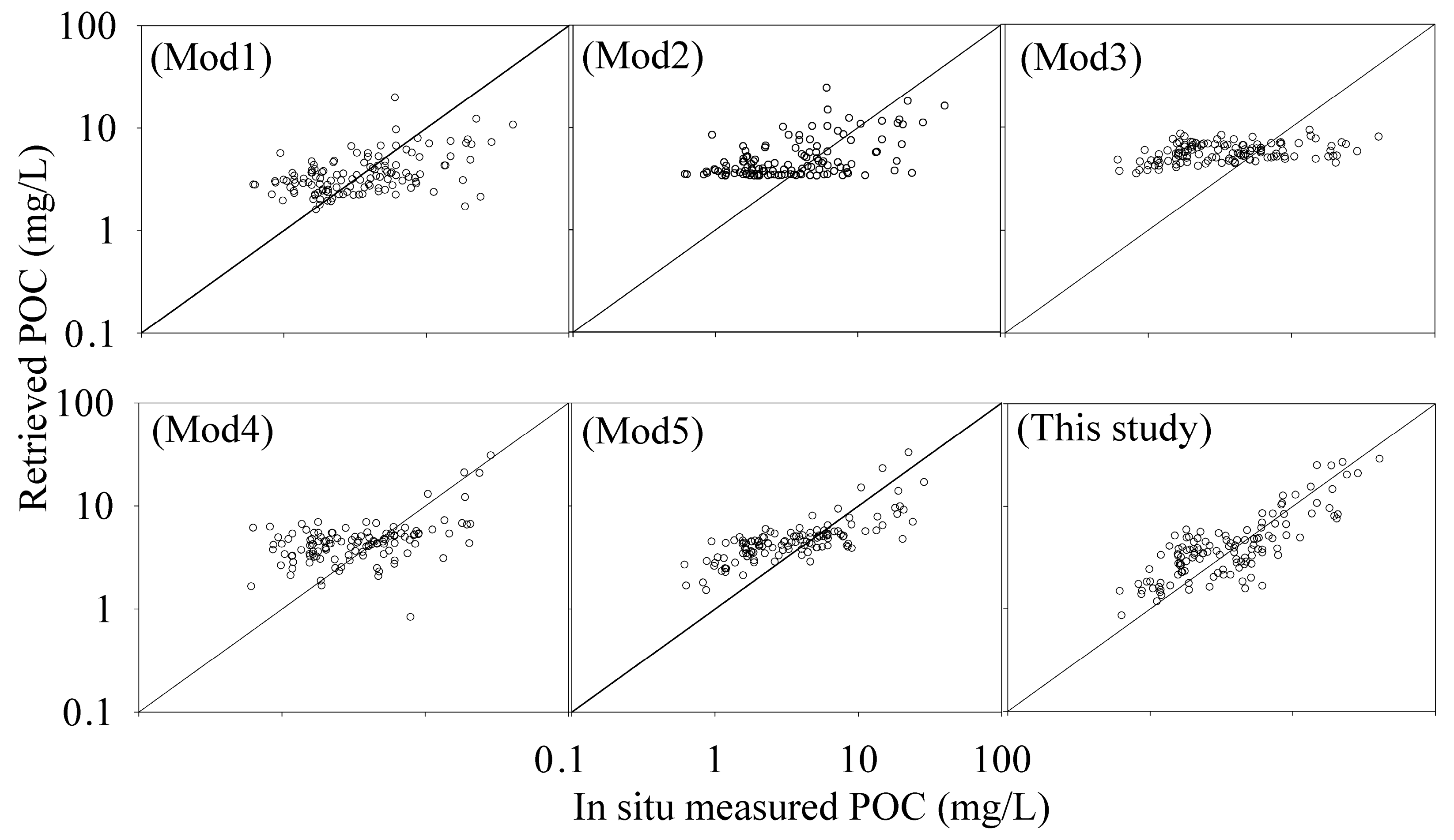
Figure 1. Study area: (A) map of the land-use cover in the Taihu basin in 2000; and (B) a picture showing the sampling points at Taihu Lake for the cruises of 5 August 2014, 24 October 2014, and 21 May 2015’ the sample sites of 10 June 2015 and 15 July 2015 are same as 21 May 2015. The segments of the lake include Meiliang Bay (MLB); Gonghu Bay (GHB); East Bay (EB); and the central (CL), northwestern (NWL), southwestern (SWL) and eastern (EL) parts of the lake.
Remotesensing 09 00624 g001
Figure 2. Calibration and validation of near infrared-red (NIR-Red) band ratio algorithm to the particulate organic carbon (POC) in Taihu Lake: (A) calibration results; and (B) validation results from data entirely independent of the calibration data.
Remotesensing 09 00624 g002
Figure 3. (A) Atmospheric correction result for the comparison of in situ measured remote sensing reflectance (Rrs) (dot dashed line) and Moderate Resolution Imaging Spectroradiometer (MODIS) -derived Rrs (dot solid line), the dotted line with the same color is the pair of measured and corrected Rrs, and the high reflectance at 859 nm is induced by extremely high amounts of phytoplankton; (B) the atmospheric correction result for the comparison of in situ measured Rrs and MODIS-derived Rrs at specific bands (645 nm and 859 nm); and (C) validation results for the MODIS-derived particulate organic carbon (POC) of match-up points.
Remotesensing 09 00624 g003
Figure 4. Annual variations in particulate organic carbon (POC) in Taihu Lake. Annual mean value of POC is the mean value for all images each year, from 2002 to 2014. The POC retrieval result in East Lake and East Bay is invalidated and should not be treated as a real distribution of POC (masked by stripe in first map).
Remotesensing 09 00624 g004
Figure 5. Annual variations in particulate organic carbon (POC) in Taihu Lake. Annual mean value of POC is the mean value for all images each year, from 2002 to 2014. The POC retrieval result in East Lake and East Bay is invalidated and should not be treated as a real distribution of POC (masked by stripe in the first map).
Remotesensing 09 00624 g005
Figure 6. Monthly particulate organic carbon (POC) variations from June 2002 to April 2014 for the mean value of Taihu Lake. The POC retrieval result in East Lake and East Bay is invalidated and did not participate in the analysis of monthly POC variations. The boundary of the box is the 25% and 75% position of POC, the line in the box is the median of POC, and the boundary of the line beside the box is the minimum and maximum value of POC.
Remotesensing 09 00624 g006
Figure 7. Monthly particulate organic carbon (POC) variations from June 2002 to April 2014 for the mean value of Taihu Lake. The POC retrieval result in East Lake and East Bay is invalidated and did not participate in the analysis of monthly POC variations. The boundary of the box is the 25% and 75% position of POC, the line in the box is the median of POC, and the boundary of the line beside the box is the minimum and maximum value of POC.
Remotesensing 09 00624 g007
Figure 8. Comparison of measured and retrieved particulate organic carbon (POC) for previous POC estimation algorithms. The information of Mod1, Mod2, Mod3, Mod4 and Mod5 are listed in Table 1.
Remotesensing 09 00624 g008
Figure 9. Relationship between particulate organic carbon (POC) and optical activity matter: (A) Chlorophyll-a (Chl-a); and (B) Suspended particulate matter (SPM) for different RE ranges.
Remotesensing 09 00624 g009
Figure 10. Evaluation of the empirical model applicability for different dominant water constituents. The data include 21 samples (red circle) from Duan et al. [33] and 14 samples (blue box) from Jiang Duan et al. [32].
Remotesensing 09 00624 g010
Figure 11. (A) Distribution of particulate organic carbon/chlorophyll-a (Chl-a) (POC/Chl-a) and particulate organic carbon/suspended particulate matter (POC/SPM) for all sampling points; and (B) correlation coefficients for POC and water constituents: phycocyanin (PC), Chl-a, SPM, organic suspended matter (OSM), and inorganic suspended matter (ISM) dissolved organic carbon (DOC), absorption coefficient of CDOM at 440 nm (aCDOM(440)), total phosphorus (TP), and total nitrogen (TN). The number of samples in the statistic analysis is 197. ** means 0.001 significance level (p < 0.001), * means 0.01 significance level (p < 0.01).
Remotesensing 09 00624 g011
Figure 12. Time-series of T, W, and P to particulate organic carbon (POC) from June 2002 to April 2014 for each lake segment (T is temperature (°C), P is precipitation (mm), and W is wind speed (m/s)).
Remotesensing 09 00624 g012
Table 1. Summary of error statistics for particulate organic carbon (POC) algorithms. All the parameters in the algorithms were re-calibrated by POC and remote sensing reflectance (Rrs) data collected from Taihu Lake.
ReferencesVariablesR2RMSPRE-RangeM|RE| ± STDEV
Mod1 Rrs(443)/Rrs(555)0.2196%−0.91~5.060.64 ± 0.71
(Stramski et al., 2008)
Mod2 (Rrs(443) − Rrs(555))/(Rrs(555) + Rrs(443))0.27141%−0.85~7.910.93 ± 1.06
(Son et al., 2009)
Mod3 Rrs(678)/Rrs(488)Rrs(748)/Rrs(412)0.05169%−1.45~5.341.21 ± 1.17
(Liu et al., 2015)
Mod4 * (Rrs(859) − Rrs(900))/(Rrs(645) − Rrs(900))0.49148%−0.79~8.800.83 ± 1.22
(Duan et al., 2014)
Mod5 Rrs(779) Rrs(709)/Rrs(620)0.5085%−0.76~3.810.63 ± 0.56
(Jiang et al., 2015)
This studyRrs(859)/Rrs(645)0.7451%−0.72~1.740.41 ± 0.29
R2 is the linear determined coefficient between measured and estimated POC, RE is the relative error, calculated by RE = (POCr − POCm)/POCm, M|RE| is the mean value of the absolute value of RE, RMSP is root mean square error percentage and STDEV is standard deviation. For Mod4*, Rrs(1240) in Duan and coworkers’ [33] algorithm is out of our FieldSpec spectroradiometer (ASD, 350–1050 nm range) measurement range, thus Rrs(900) was used instead of Rrs(1240) in this study.
Table 2. Water constituents for different accuracy ranges retrieved by particulate organic carbon (POC) estimation algorithm. The value in the bracket is the mean value of each water constituent in the range above it.
Model ErrorChl-aSPMISMOSMPOCaCDOM(440)
(RE)(μg/L)(mg/L)(mg/L)(mg/L)(mg/L)(m−1)
>50%7.4–181.210.7–101.36.1–87.94.6–21.40.6–2.30.6–6.9
(37.16)(39.46)(30.31)(9.15)(1.55)(3.73)
25%–50%5.6–301.06.9–105.72–92.14.9–19.70.9–14.750.3–7.9
(44.10)(54.23)(43.89)(10.34)(2.35)(2.56)
−25%–25%7.5–343.710.9–107.53.9–89.35.1–45.80.6–23.950.4–8.2
(72.10)(43.57)(30.80)(13.41)(5.67)(2.60)
<−25%28.3–431.514.2–249.82.2–90.55–224.82.6–40.550.3–8.0
(119.77)(52.80)(29.01)(24.63)(9.27)(2.49)
Table 3. Correlation coefficients of particulate organic carbon (POC) to T, W, P and autocorrelation coefficients of POC for each lake segment (T is temperature (°C), P is precipitation (mm), and W is wind speed (m/s)); the number of samples in the statistical analysis is 197.
Lake SegmentsCLGBMLBNWLSWLTB
CL1
GB0.551
MLB0.440.76 1
NWL0.78 0.640.621
SWL0.82 0.400.210.651
TB0.90 0.750.640.91 0.781
T−0.030.490.600.41−0.220.32
W0.210.06−0.160.110.230.12
P0.130.290.300.220.240.17

