Remote Sensing Image Registration Using Multiple Image Features

Abstract

Remote sensing image registration plays an important role in military and civilian fields, such as natural disaster damage assessment, military damage assessment and ground targets identification, etc. However, due to the ground relief variations and imaging viewpoint changes, non-rigid geometric distortion occurs between remote sensing images with different viewpoint, which further increases the difficulty of remote sensing image registration. To address the problem, we propose a multi-viewpoint remote sensing image registration method which contains the following contributions. (i) A multiple features based finite mixture model is constructed for dealing with different types of image features. (ii) Three features are combined and substituted into the mixture model to form a feature complementation, i.e., the Euclidean distance and shape context are used to measure the similarity of geometric structure, and the SIFT (scale-invariant feature transform) distance which is endowed with the intensity information is used to measure the scale space extrema. (iii) To prevent the ill-posed problem, a geometric constraint term is introduced into the L2E-based energy function for better behaving the non-rigid transformation. We evaluated the performances of the proposed method by three series of remote sensing images obtained from the unmanned aerial vehicle (UAV) and Google Earth, and compared with five state-of-the-art methods where our method shows the best alignments in most cases.

1. Introduction

Remote sensing image registration refers to the fundamental task in image processing to align two or more images of the same scene (i.e., the sensed images and the reference images), which can be multiview (obtained from different viewpoint), multitemporal (taken at different times) and multisource (derived from different sensors). In this paper, we mainly focus on registering the remote sensing images taken from different viewpoint. As a basic technology in the field of remote sensing image processing, it has been widely used in the field of military and civilian such as natural disaster damage assessment, resource census, assignment of climate changes, military damage assessment, environment monitoring and ground targets identification, etc.

Existing remote sensing image registration methods can be approximately classified into two categories: area-based methods and feature-based methods. Various reviews on image registration methods can be found in [1,2,3,4,5]. Area-based methods use the pixel intensities of identical image windows to estimate similarity while feature-based methods extract image features (e.g., points, lines, and regions) and match them using similarity criteria [6]. When there are noises, complex distortion and significant radiometric differences between the images to be aligned, the computation complexity or the search space of the area-based methods will increase nonlinearly with the transformation complexity and feature-based methods are more robust and preferable. In this paper, the captured remote sensing images exist the local non-rigid geometric distortions caused by ground relief variations and imaging viewpoint changes, thus we mainly focus on feature-based methods for registration. Such methods generally consists of three steps [7]: (i) feature descriptors extraction; (ii) feature point sets registration; (iii) image transformation and resampling.

Generally, a good feature descriptor should be distinctive and at the same time robust to changes in viewing conditions as well as to errors of the point detector [8]. For desirable local image descriptors, to improve distinctiveness while maintaining robustness is the main concern [9]. Among the popular local invariant features which have been proposed in remote sensing image registration (e.g., Harris [10], scale-invariant feature transform (SIFT) [11,12] and speeded-up robust features (SURF) [13]), Mikolajczyk et al. [8] demonstrated that the performance of SIFT [11] under affine transformation, scale change, rotation, image blur, jpeg compression, and illumination change outperforms other local invariant descriptors in most of the tests. There are various researches for remote sensing image registration based on the variants of SIFT algorithm or the combination of SIFT and some other algorithms. Li et al. [14] proposed a new criterion named scale-orientation joint restriction criteria in order to overcome the intensity difference between remote sensing image pairs. Sedaghat et al. [6] introduced an automatic registration algorithm by extracting high-quality SIFT features in the uniform distribution of both the scale and image spaces. In addition, other variants of SIFT such as PCA-SIFT [15], SAR-SIFT [16], AB-SIFT [17] and SIFT-DRS [18] are also proposed in literatures. Furthermore, Goncalves et al. [19] developed a new AIR (Automatic image registration) method based on the combination of image segmentation and SIFT, and the method is complemented by a robust procedure of outlier removal. In [20], a novel coarse-to-fine scheme for automatic image registration based on SIFT and MI is proposed, and their method achieved the outlier removal and also can generally reject most incorrect matches.

Feature-based methods are typically formulated as a point set registration problem, since point representations are general and easy to extract. In order to achieve a robust point registration, it is crucial to construct putative correspondences based on local invariant feature similarity at first and then estimate the spatial transformation based on geometric structure feature constraint [21,22,23]. Here, we briefly review some point set registration methods since our method is based on feature point. Fischler et al. proposed the classical random sample consensus (RANSAC) [24] algorithm. Myronenko and Song [25] introduced a probabilistic method, called the coherent point drift (CPD) algorithm, for both rigid and non-rigid point set registration. Moreover, Liu and Yan [26] investigated how to discover common visual pattern discovery via spatially coherent correspondences and recover the correct correspondences. Zhang et al. [27] defined the spatially consistent topic model by making full use of the correlation between image classification and annotation. Recently, Ma et al. proposed a robust $L_2$-minimizing estimate ($L_{2}E$) [28] for non-rigid point set registration, they later proposed a flexible and general algorithm called locally linear transforming (LLT) [29] for both rigid and non-rigid registration on remote sensing images. More recently, Yang et al. [30] proposed a new method named GLMDTPS, which considers global and local structural differences as a linear assignment problem.

Although the aforementioned methods have been proposed for different applications, there still exists the following problems for remote sensing image registration. (i) These methods use either the local invariant features or geometric features, thus the distinctiveness capability of the feature points is lost in the complex remote sensing registration patterns. For example, methods for image registration which use only SIFT [11,12] or its variants [6,14,15,16,17,18,19,20] suffer from inaccurate registration of SIFT. In addition, the performances of the methods [23,24,25,26,27,28,29,30] which consider only the geometric structure features is limited by the assumption that the corresponding points have similar structures. (ii) Using a rigid or affine transformation model is infeasible for registering remote sensing images with different viewpoints since the images usually contain local non-rigid distortion. (iii) It is ill-posed for mapping one feature point set to another by a non-rigid transformation model since the solution is not unique.

In this paper, we present a new method for remote sensing image registration with different viewpoints. Compared with the current methods, the major differences and advantages of this paper are as follows. (i) Probabilistic model construction: the mixture-feature Gaussian mixture model (MGMM) is constructed for simultaneously dealing with different types of image features. (ii) Feature complementation: Making the respective advantages of Geometric structure and intensity information to complement each other, i.e., the Euclidean distance and shape context to measure the similarity of global and local geometric structure discrepancies, and the SIFT distance to measure the scale space extrema, both of which are combined and substituted into the mixture model by which the reliable correspondence is obtained. (iii) Geometric constraint: a regularization term to prevent the ill-posed problem based on coherent velocity field is introduced into the L2E-based energy function for better behaving the non-rigid transformation.

The rest of this paper is organized as follows. Section 2 introduces our method in detail. Section 3 demonstrates the registration performance of our method on various types of remote sensing images with different viewpoints against other methods, followed by some concluding remarks in Section 4.

2. Methodology

We first introduce the three major contributions of the proposed method: (i) modeling of the MGMM; (ii) feature specification and combination; and (iii) geometric constrained energy function. Whereafter the main process is demonstrated, followed by the method analysis.

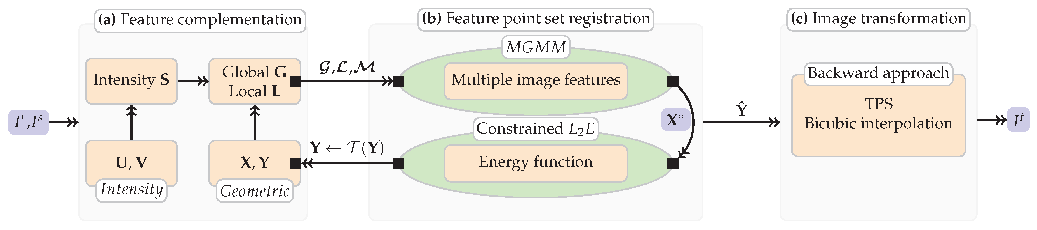
2.1. Mixture-Feature Gaussian Mixture Model (MGMM)

The motivation behind the development of MGMM is the need for estimating reliable correspondence using multiple image features whereas the Gaussian mixture model (GMM) can only work on single feature. In this subsection we detail the derivation of the MGMM.

Based on the reasonable assumption that points from one set are normally distributed around points belonging to the other set, we therefore consider the registration of two point sets as a GMM probability density estimation problem. Let ${\mathbf{y}}_j$ be the centroid of the $j^{th}$ Gaussian component, ${\mathbf{x}}_i$ the $i^{th}$ data. The probability density function (PDF) is obtained as:

$$p\left({\mathbf{x}}_i\right)=(1-\zeta )\sum _{j=1}^m{\mathcal{C}}_{ij}p\left({\mathbf{x}}_i\right|{\mathbf{y}}_j)+\zeta \frac{1}{n},$$

(1)

where $p\left({\mathbf{x}}_i\right|{\mathbf{y}}_j)=\frac{1}{{\left(2\pi {\sigma }^2\right)}^{\frac{d_e}{2}}}exp\left(-\frac{\parallel {\mathbf{x}}_i-{\mathbf{y}}_j{\parallel }^2}{2{\sigma }^2}\right)$ with the equal isotropic covariances ${\sigma }^2$ shared, ${\mathcal{C}}_{ij}=\frac{1}{m}$ are nonnegative equal quantity with ${\sum }_{j=1}^m{\mathcal{C}}_{ij}=1$, which are called the priors of the GMMs. $\frac{1}{n}$ is an additional uniform distribution with a weighting parameter $\zeta$, $0\le \zeta \le 1$ for outlier dealing. However, $p\left({\mathbf{x}}_i\right|{\mathbf{y}}_j)$ considers only the Euclidean distance and might lead to insufficient robustness in some registration scenarios, e.g., although the local structure around ${\mathbf{x}}_a$ and ${\mathbf{x}}_b$ are different, $p\left({\mathbf{x}}_a\right|{\mathbf{y}}_j)=p\left({\mathbf{x}}_b\right|{\mathbf{y}}_j)$ if $\parallel {\mathbf{x}}_a-{\mathbf{y}}_j{\parallel }^2={\parallel {\mathbf{x}}_b-{\mathbf{y}}_j\parallel }^2$.

Consequently, the MGMM which is capable of dealing with multiple image features is developed. The PDF of the MGMM is formulated as:

$$f\left({\mathbf{x}}_i\right)=(1-\zeta )\sum _{j=1}^m{\mathcal{M}}_{ij}f\left({\mathbf{x}}_i\right|{\mathbf{y}}_j)+\zeta \frac{1}{n},$$

(2)

where $f\left({\mathbf{x}}_i\right|{\mathbf{y}}_j)=\frac{1}{{\left(2\pi {\sigma }^2\right)}^{\frac{d_e}{2}}}exp\left[-\left({\mathcal{G}}_{ij}+\alpha {\mathcal{L}}_{\mathit{ij}}\right)\right]$ and $\alpha$ is a constant. ${\mathcal{G}}_{m\times n}$ and ${\mathcal{L}}_{m\times n}$ exploit the global and local geometric structure discrepancies, priors ${\mathcal{M}}_{m\times n}$ are specified by measuring the discrepancy of intensity information, which is analogous to confidence.

Once we have the PDF of the MGMM, the correspondence between the two point sets can be easily inferred through the posterior probability of the MGMM which is written as:

$$p_{ij}=\frac{{\mathcal{M}}_{ij}f\left({\mathbf{x}}_i\right|{\mathbf{y}}_j)}{{\sum }_{k=1}^m{\mathcal{M}}_{ik}f\left({\mathbf{x}}_i\right|{\mathbf{y}}_k)+\zeta \frac{1}{n}},$$

(3)

where ${\mathbf{P}}_{m\times n}$ is the posterior probability matrix by which the newly estimated coordinates of ${\mathbf{x}}_i$ can be obtained. It is worth nothing that two strategies for constraining $\mathbf{P}$ are herein under consideration: (i) a single normalization enforcing ${\sum }_{j=1}^m{p}_{ij}=1$ and (ii) a double normalization which additionally requires ${\sum }_{i=1}^n{p}_{ij}=1$. Intuitively, the former acts like an one-to-many correspondence estimation, whereas the latter provides an one-to-one counterpart. In our method, the number of the feature points are strictly equal because the applied SIFT feature extractor. In addition the outlier to data ratios, however, are unknown and varied due to the different overlap ratios of each image pair. In this case it is inappropriate for requiring an one-to-one correspondence since the presence of outliers might trap the estimation, whereby the first strategy is chosen in this paper.

2.2. Combination and Complementation of Multiple Image Features

The distinctiveness of feature points, which affects the accuracy of the feature matching, are mainly determined by the robustness of the involved measures. However, different types of measures have their own advantages and limitations, where our idea is to make their respective advantages complementary to each other. In order to make the paper more self-contained, we succinctly discuss the concept of the three features we used, i.e., the Euclidean distance, the SC and the SIFT distance. The combination of features and the complete form of posterior probability function Equation (3) are then discussed.

2.2.1. Euclidean Distance

The squared Euclidean distance of ${\mathbf{x}}_i$ and ${\mathbf{y}}_j$ is simply written as:

$$g_{ij}={\parallel {\mathbf{x}}_i-{\mathbf{y}}_j\parallel }^2.$$

(4)

It acts a straightforward global estimation with insufficient robustness in many scenarios. To alleviate this problem, $g_{ij}$ is commonly treated as an argument of a Gaussian function, which therefore plays a flexible global estimation by the help of the changeable covariances.

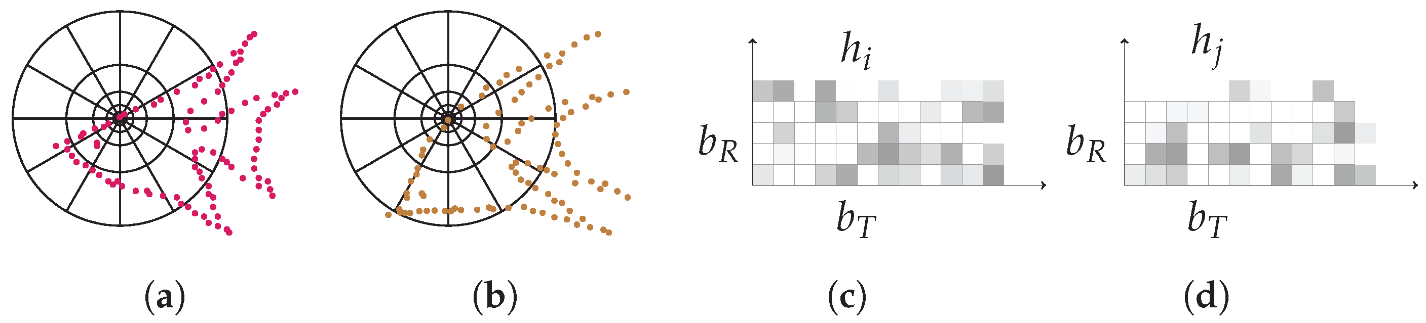
2.2.2. Shape Context (SC)

The work in [31,32] proposed the SC. A detailed illustration of the SC is shown in Figure 1. The SC constructs a polar coordinate with $B_R$ bins in the radial direction and $B_T$ bins in the tangential direction, by centering the polar coordinate at ${\mathbf{x}}_i$ and ${\mathbf{y}}_j$, it counts the number of points within each bin and obtains two $1\times B$ sets ${\left\{h_i\left(b\right)\right\}}_{b=1}^B$ and ${\left\{h_j\left(b\right)\right\}}_{b=1}^B$, respectively, where $B=B_R\times B_T$. The SC discrepancy of ${\mathbf{x}}_i$ and ${\mathbf{y}}_j$ is measured using Chi-square distribution as:

$$l_{ij}=\frac{1}{2}\sum _{b=1}^B\frac{{[h_i\left(b\right)-h_j\left(b\right)]}^2}{h_i\left(b\right)+h_j\left(b\right)}.$$

(5)

The SC is robust especially in scenarios like contour point set registration and hand-written characters matching, etc., because the geometric structure of these shapes are quite distinctive. However, it can also be deteriorated if ${\mathbf{x}}_i$ and ${\mathbf{y}}_j$ have similar neighborhood structure.

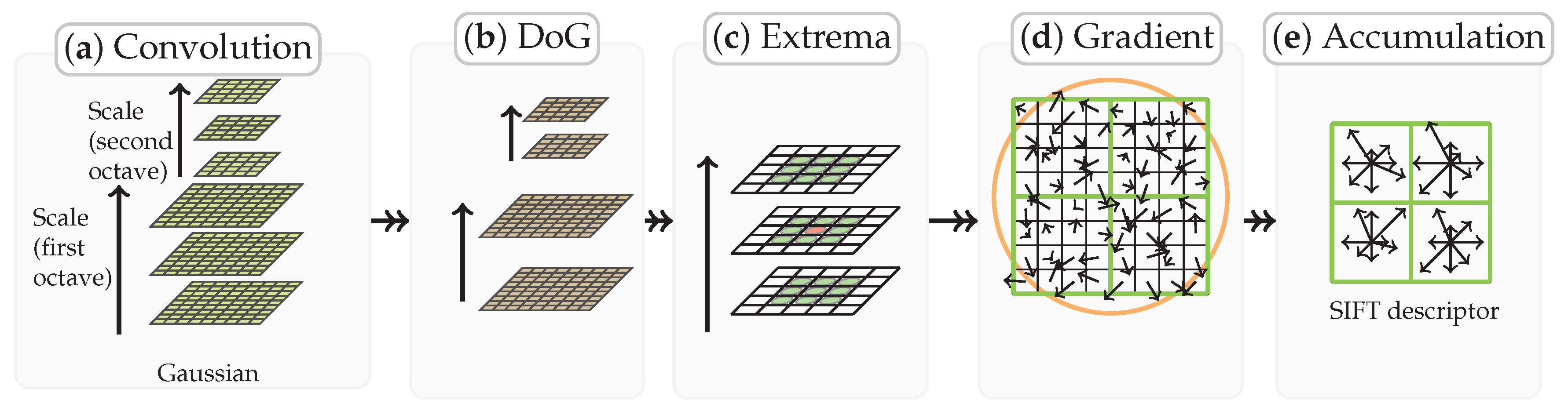
2.2.3. SIFT Distance

The SIFT algorithm introduced by Lowe is a classic algorithm, it first repeatedly convolves the images with Gaussians to produce the set of scale space images and obtains the difference-of-Gaussian images. The feature points are detected by comparing a pixel with its neighbors at the current and adjacent scales. Histograms of local oriented gradients around each feature points are then computed, obtaining an 128-dimensional vector as the SIFT descriptor, as shown in Figure 2. Finally, a process for matching the feature points are carried out. A matching pair is detected, if its distance is closer than $\tau$ times the distance of the second nearest neighbor. Thus, the feature points extracted from the sensed and reference images are of the same number, i.e., $\left|\mathbf{X}\right|=\left|\mathbf{Y}\right|$, where $|·|$ denotes the cardinality of a set, and each pair with the same suffix are matched already from the view of intensity information.

The SIFT distance is defined as:

$$s_{ij}={\parallel {\mathbf{u}}_i-{\mathbf{v}}_j\parallel }^2,$$

(6)

where $\mathbf{S}$ is of $m\times n$ dimension. ${\mathbf{u}}_i$ and ${\mathbf{v}}_j$ are the SIFT descriptors of ${\mathbf{x}}_i$ and ${\mathbf{y}}_j$, respectively. We have introduced three relevant features of our method, i.e., $\mathbf{G}$, $\mathbf{L}$ and $\mathbf{S}$. The next concern is to substitute them into our MGMM.

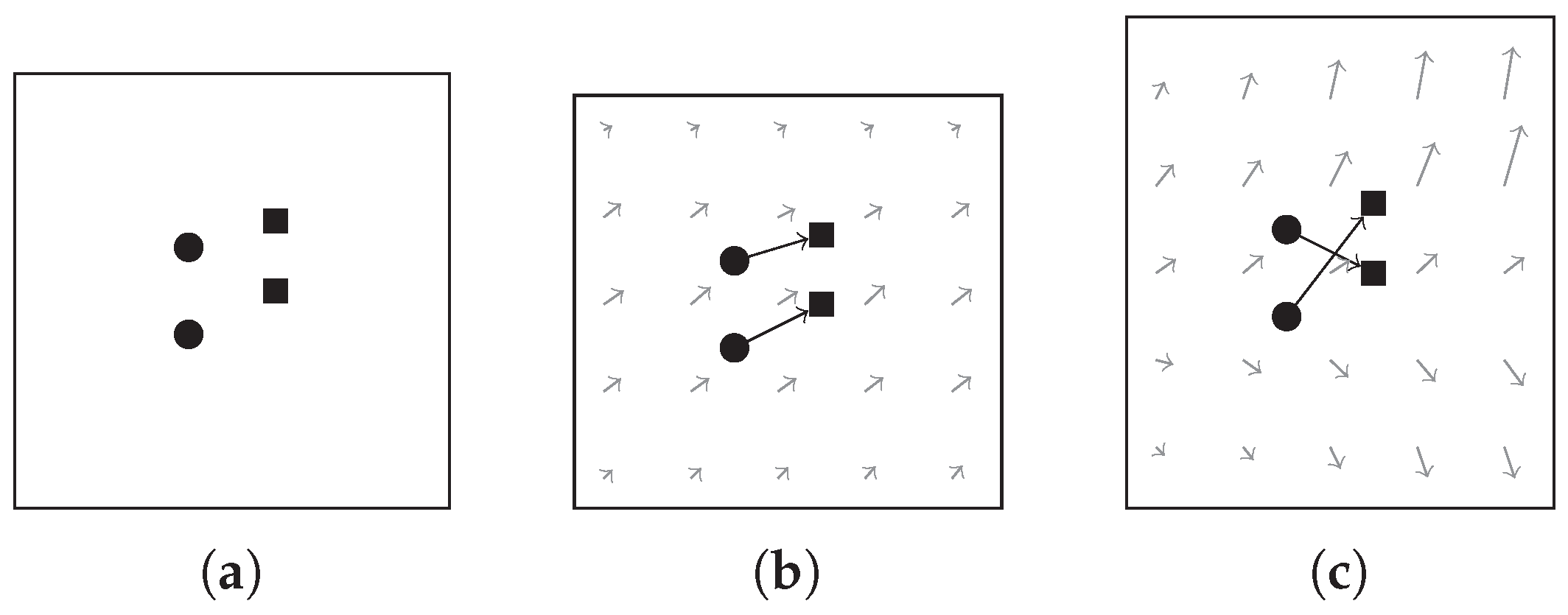
2.2.4. Multiple Image Feature Based Correspondence Estimation

The global geometric feature discrepancy are defined by ${\mathcal{G}}_{ij}=\frac{g_{ij}}{2{\sigma }^2}$, where ${\sigma }^2$ are the covariances of the MGMM. It actually forms the Gaussian function of the pairwise Euclidean distance in the context of $f\left({\mathbf{x}}_i\right|{\mathbf{y}}_j)$. The local geometric feature discrepancy ${\mathcal{L}}_{ij}$ are defined as the Chi-square distribution of the SC histograms, i.e., ${\mathcal{L}}_{ij}=l_{ij}$. The Priors of the MGMMs are formulated as ${\mathcal{M}}_{ij}=1-{\tilde{s}}_{ij}$, where matrix $\tilde{\mathbf{S}}$ is obtained by row-by-row rescaling which makes each entry ${\tilde{s}}_{ij}\in [0,1]$, and are therefore taken as the confidence. Substituting ${\mathcal{G}}_{ij}$, ${\mathcal{L}}_{ij}$ and ${\mathcal{M}}_{ij}$ into Equation (3), we can therefore rewrite it as:

$$p_{ij}^{*}=\frac{(1-{\tilde{s}}_{ij})exp\left[-\left(\frac{g_{ij}}{2{\sigma }^2}+\alpha l_{ij}\right)\right]}{{\sum }_{k=1}^m(1-{\tilde{s}}_{ik})exp\left[-\left(\frac{g_{ik}}{2{\sigma }^2}+\alpha l_{ik}\right)\right]+{\left(2\pi {\sigma }^2\right)}^{\frac{d_e}{2}}\frac{\zeta }{n}}.$$

(7)

The underlying assumption of density function Equation (7) is the decomposition of the process for human to recognize and categorize objects. Supposing such process is based on the linear combination among features such as Euclidean distance and density, etc. The priority of certain features may change during the process. For instance, one can easily categorize different letters according to the feature of shape at the very beginning, whereafter the accuracy can be further optimized by involving other features in. Following this idea, an deterministic annealing scheme is applied to control the fuzziness, which progressively decreases the covariances by ${\sigma }^2\leftarrow ϵ{\sigma }^2$ from a large value, where $ϵ$ is a constant. In the early stage of iterations, the two point sets have the biggest difference, estimation based on Euclidean distance is less accurate, yet the local geometric feature discrepancy and the intensity information are relative strong and stable. The unreliable global correspondence is filtered due to the property of negative nature exponential function. At the final stage of iterations, ${\mathbf{x}}_i$ and ${\mathbf{y}}_j$ are very similar, a direct estimation using the global geometric feature is desirable. In addition, the statuses of these features interchange as ${\sigma }^2$ is small, leading to binary-like correspondences.

Furthermore, the correspondences estimation of the MGMM is a fuzzy-to-binary process, by which the correspondences are able to be improved gradually and continuously during the optimization without jumping around in the space of binary permutation matrices.

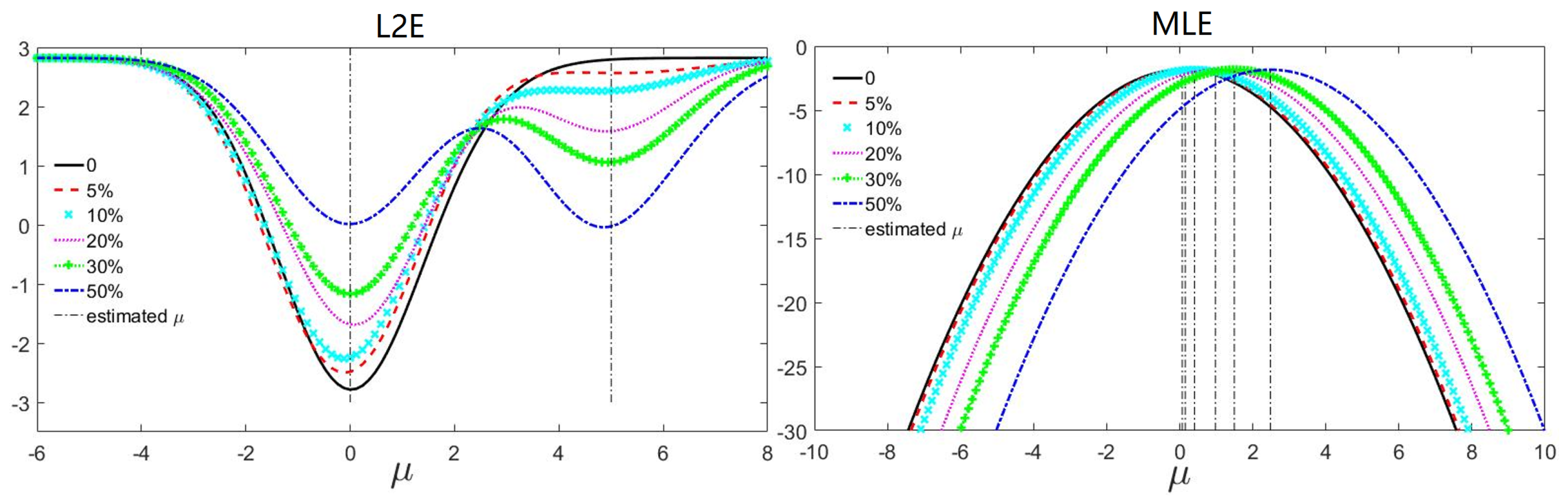
2.3. Geometric Constraint for L2E Based Energy Optimization

Based on the reliable correspondence estimated by the MGMM, the target coordinate is determined by ${\mathbf{x}}_i^{*}={\sum }_{j=1}^n{p}_{ij}{\mathbf{x}}_j$. Our next concern is to formulate a criterion, by which a reasonable position $\mathcal{T}\left({\mathbf{y}}_i\right)$ of ${\mathbf{y}}_i$ is determined. This position in turn improves the accuracy of the correspondence estimation in the next iteration interlockingly. In this subsection, we formulate the L2E based energy function with geometrical constraint. Followed by sketching out the related concepts and techniques, i.e., the $L_2$-minimizing estimate ($L_{2}E$) and the motion coherent based geometric constraint.

The unknown coordinates of the source point set to be transformed is estimated by using the L2E based energy function with geometric constraint which is written as:

$$\mathcal{Q}(\mathcal{T},{\rho }^2)=L_{2}E(\mathcal{T},{\rho }^2)+\frac{\lambda }{2}\mathcal{R}\left(\mathcal{T}\right),$$

(8)

where $\mathcal{T}$ is the non-rigid transformation, ${\rho }^2$ is the parameter of the density models we used to represent the deviation between the source and target point sets, $L_{2}E(·)$ is the L2E estimator and $\mathcal{R}(·)$ is the geometric constraint on $\mathcal{T}$ based on the Tikhonov regularization theory [33], the constant $\lambda$ controls the strength of the constraint.

2.3.1. $L_{2}E$

$L_{2}E$ [34] is a robust estimator which minimizes the $L_2$ distance between densities, and is particularly appropriate for analyzing massive datasets where outlier rejecting is impractical.

Suppose we have a density model $p\left(z\right|\theta )$, our goal is to minimize the estimate of $L_2$ distance with respect to $\theta$ as ${\theta }^{*}={arg\; min}_{\theta }\int {\left[p\left(z\right|\theta )-p\left(z\right|{\theta }_0)\right]}^{2}dz$, where the true parameter ${\theta }_0$ is unknown. After omitting the constant $\int p{\left(z\right|{\theta }_0)}^2$dz, parameter $\theta$ is estimated by minimizing the $L_{2}E$ criterion as:

$${\theta }_{L_{2}E}^{*}=\underset{\theta }{arg\; min}\left[\int p{\left(z\right|\theta )}^{2}dz-\frac{2}{m}\sum _{i=1}^{m}p\left(z\right|\theta )\right].$$

(9)

The robustness of the L2E estimator can be shown by comparing against the maximum log-likelihood estimator (MLE). Consider a sample of size 500 from a normal distribution $\mathcal{N}(0,1)$ which stands for the inliers, five normal distributed samples $\mathcal{N}(5,1)$ in a tendency of increasing size (e.g., 25, 50, 100, 150, 250) act as outliers. The estimated means are shown in Figure 3. $L_{2}E$ has a stable global minimum at approximately 0, as well as a local minimum at approximately 5 which becomes deeper as the number of outliers increases. This is reasonable since the outliers are from $\mathcal{N}(5,1)$. By contrast, MLE is not resistant to outliers, since the global minimum deviates more under heavier contamination.

2.3.2. Motion Coherent Based Geometric Constraint

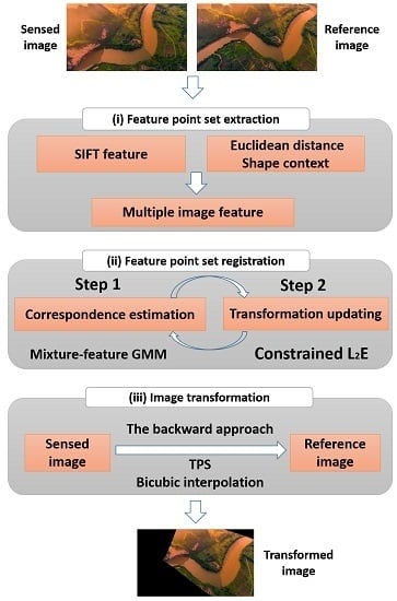
The key constraint of a rigid transformation is that all distances are preserved. However, once non-rigidity is allowed, there are an infinite number of ways to map one point set onto another. An appropriate constraint is necessary to solve this ill-posed problem. To this end, the motion coherent based geometric constraint is introduced into our method.

In motion perception, there are a number of important phenomena involving coherence. Velocity coherence is a particular way of imposing smoothness on the underlying transformation. The concept of motion coherence is proposed in the motion coherence theory [35] which is intuitively interpreted as that points close to one another tend to move coherently. Examples of velocity fields with two different levels of motion coherence for two different point correspondences are illustrated in Figure 4. Since our focus is on its application in remote sensing image registration, we will not drill-down further into the theoretical model but directly write the geometric constraint $\mathcal{R}\left(\mathcal{T}\right)$ in the form as:

$$\mathcal{R}\left(\mathcal{T}\right)={\parallel \mathcal{T}\parallel }^2$$

(10)

It implies that we are imposing motion coherence among the SIFT feature points, and discouraging the undesired transformation, e.g., as shown in Figure 4c, over the whole warping plane. With a large $\lambda$, the constraint produces globally smooth transformation, while it produces more arbitrary transformation with small values.

2.4. Main Process

Given a sensed image $I^s$ of size $N_w\times N_h$ and a reference image $I^r$ of size $N_w^{\prime }\times N_h^{\prime }$, our goal is to obtain a transformed image $I^t$ of size $N_w^{\prime }\times N_h^{\prime }$ by recovering the underlying geometric transformation from $I^s$ to $I^r$. The main process of our method consists of three steps as shown in Figure 5: (i) extraction of the feature point sets, (ii) registration of the extracted feature point sets, and (iii) image Transformation and resampling, where the second step comprises an alternating two-step process: correspondence estimation and transformation updating of the feature point sets.

2.4.1. Extraction of the Feature Point Sets

SIFT algorithm is employed for feature point sets extraction. By $\{{\mathbf{Y}}_{m\times d_e},{\mathbf{V}}_{m\times d_s}\}$ and $\{{\mathbf{X}}_{n\times d_e},{\mathbf{U}}_{n\times d_s}\}$ we denote the feature point sets and SIFT descriptor sets extracted from the sensed and reference images, respectively, where $\mathbf{Y}={\{{\mathbf{y}}_1,{\mathbf{y}}_2,...,{\mathbf{y}}_m\}}^T$ and $\mathbf{X}={\{{\mathbf{x}}_1,{\mathbf{x}}_2,...,{\mathbf{x}}_n\}}^T$ are the $d_e$ dimensional geometrical coordinates of the source and target point sets , and $\mathbf{V}={\{{\mathbf{v}}_1,{\mathbf{v}}_2,...,{\mathbf{v}}_m\}}^T$ and $\mathbf{U}={\{{\mathbf{u}}_1,{\mathbf{u}}_2,...,{\mathbf{u}}_n\}}^T$ are the intensity information, namely the $d_s$ dimensional SIFT descriptors for $\mathbf{X}$ and $\mathbf{Y}$, respectively. Note that $\mathcal{T}\left(\mathbf{Y}\right)$ (initial $\mathcal{T}\left(\mathbf{Y}\right)=\mathbf{Y}$) denotes the transformed set $\mathbf{Y}$ in each iteration, and a general derivation is realized by using different suffixes n and m where $m=n$ actually.

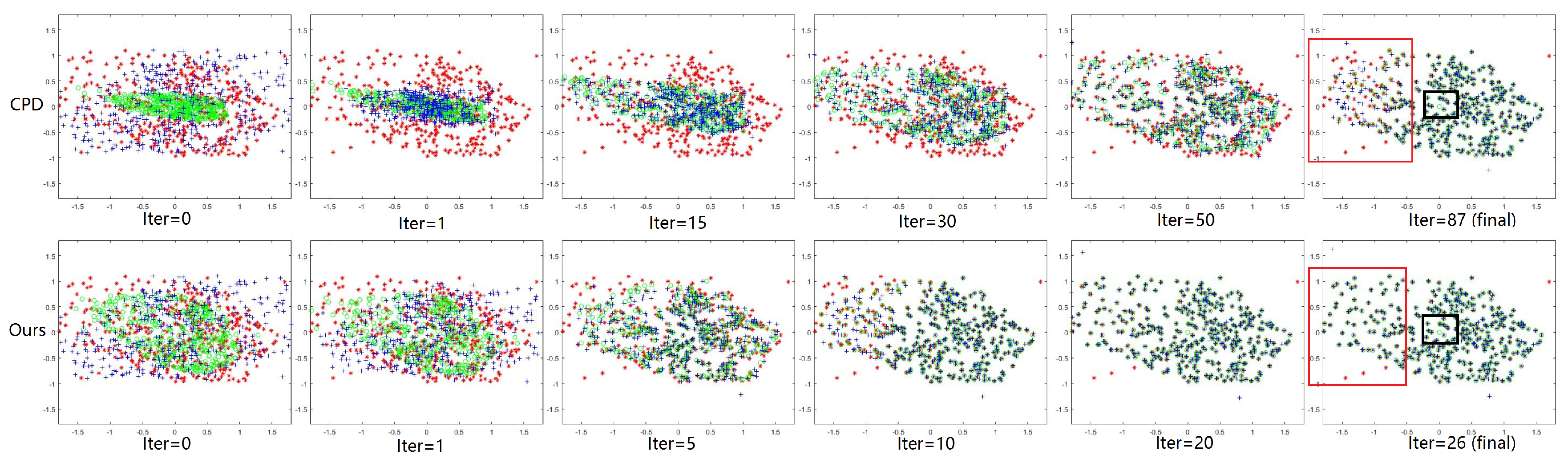
2.4.2. Feature Point Set Registration

Correspondence estimation: The pairwise global and local geometric structure discrepancies $\mathbf{G}$ and $\mathbf{L}$, and the SIFT distance $\mathbf{S}$ are obtained by Equations (4)–(6), respectively. The posterior probability matrix, which is also known as the correspondence matrix is then written as:

$$p_{ij}^{*}=\frac{(1-{\tilde{s}}_{ij})exp\left[-\left(\frac{\parallel {\mathbf{x}}_i-{\mathbf{y}}_j{\parallel }^2}{2{\sigma }^2}+\frac{\alpha }{2}{\sum }_{b=1}^B\frac{{[h_i\left(b\right)-h_j\left(b\right)]}^2}{h_i\left(b\right)+h_j\left(b\right)}\right)\right]}{{\sum }_{k=1}^m(1-{\tilde{s}}_{ik})exp\left[-\left(\frac{\parallel {\mathbf{x}}_i-{\mathbf{y}}_k{\parallel }^2}{2{\sigma }^2}+\frac{\alpha }{2}{\sum }_{b=1}^B\frac{{[h_i\left(b\right)-h_k\left(b\right)]}^2}{h_i\left(b\right)+h_k\left(b\right)}\right)\right]+{\left(2\pi {\sigma }^2\right)}^{\frac{d_e}{2}}\frac{\zeta }{n}},$$

(11)

where ${\mathbf{P}}^{*}$ is of size $m\times n$. ${\tilde{s}}_{ij}$, ${\tilde{s}}_{ij}\in [0,1]$ is the rescaled SIFT distance, ${\sigma }^2$ are the equal covariances of the MGMM, constant $\zeta$ is the outlier weighting, and B bins are used to construct the SC log-polar coordinate. Hence, the estimated corresponding set is obtained by

$${\mathbf{X}}^{*}={\mathbf{P}}^{*}\mathbf{X}.$$

(12)

After computing ${\mathbf{X}}^{*}$, the non-rigid transformation is modeled by the current correspondence ${\mathbf{X}}^{*}$ and the source point set $\mathbf{Y}$.

Transformation updating: The Resiz representation theorem states that if $\psi$ is a bounded linear function on a Hilbert space $\mathcal{H}$, then there is a unique vector $\nu$ in $\mathcal{H}$, making $\psi t=\langle t,\nu \rangle$ for all $\psi \in \mathcal{H}$. Thus the cumbersome mapping problem reduces to find the unique vector $\nu$. This motivates us to model the non-rigid transformation $\mathcal{T}$ by requiring it to lie within the reproducing kernel Hilbert space (RKHS).

We first define a RKHS $\mathcal{H}$ by choosing a positive definite kernel, here we adopt the Gaussian kernel, which is in the form $\mathbf{\Theta }({\mathbf{y}}_i,{\mathbf{y}}_j)=exp(-\frac{1}{2{\beta }^2}\parallel {\mathbf{y}}_i-{\mathbf{y}}_j{\parallel }^2)$, where $\beta$ is a constant to control the spatial smoothness and $\mathbf{\Theta }$ is of size $m\times m$. According to the representation theorem, the optimal transformation function $\mathcal{T}$ takes the form

$$\mathcal{T}\left(\mathbf{Y}\right)=\mathbf{Y}+\mathbf{\Theta }\mathbf{W},$$

(13)

where ${\mathbf{W}}_{m\times d_e}={\{{\mathbf{w}}_1,{\mathbf{w}}_2,...,{\mathbf{w}}_m\}}^T$ is the coefficient matrix. Hence, the minimization over energy function Equation (8) boils down to finding a finite coefficients matrix $\mathbf{W}$.

The non-rigid transformation $\mathcal{T}\left(\mathbf{Y}\right)$ is equivalent to the initial position plus a displacement function i.e., $\mathcal{T}\left(\mathbf{Y}\right)=\mathbf{Y}+\mathcal{V}\left(\mathbf{Y}\right)$. It is worth nothing that $\mathcal{R}\left(\mathcal{T}\right)$ and $\mathcal{R}\left(\mathcal{V}\right)$ are exactly the same, i.e., $\mathcal{R}\left(\mathcal{T}\right)=\mathcal{R}(\mathbf{Y}+\mathcal{V}(\mathbf{Y}\left)\right)=\mathcal{R}\left(\mathcal{V}\right)$, since $\mathcal{R}\left(\mathcal{T}\right)$ is invariant under affine transformations. In this paper, we solve for $\mathcal{V}$ instead of $\mathcal{T}$. The complete energy function Equation (8) takes the form as:

$$Q(\mathbf{W},{\rho }^2)=\frac{1}{2^{d_e}{(\pi \rho )}^{\frac{d_e}{2}}}-\frac{2}{m}\sum _{i=1}^n\frac{1}{{(2\pi {\rho }^2)}^{\frac{d_e}{2}}}exp\left(\frac{{∥{\mathbf{x}}_i^{*}-{\sum }_{j=1}^m\mathbf{\Theta }({\mathbf{y}}_i,{\mathbf{y}}_j)w_j∥}^2}{2{\rho }^2}\right)+\lambda tr(\mathbf{W}\mathbf{\Theta }\mathbf{W}),$$

(14)

where constant $\lambda$ controls the strength of the constraint, $tr(·)$ denotes the trace of a matrix. Taking derivative of Equation (14) with respect to coefficient matrix $\mathbf{W}$, we obtain:

$$\frac{\partial Q}{\partial \mathbf{W}}=\frac{2\mathbf{\Theta }[\mathbf{U}\odot (\mathbf{E}\otimes \mathbf{1}\left)\right]}{m{\rho }^2{\left(2\pi {\rho }^2\right)}^{\frac{d_e}{2}}}+2\lambda \mathbf{W},$$

(15)

where ${\mathbf{U}}_{m\times d_e}=\mathbf{\Theta }\mathbf{W}-{\mathbf{X}}^{*}$, ${\mathbf{E}}_{m\times 1}=exp\{diag\left(\mathbf{U}{\mathbf{U}}^T\right)/2{\rho }^2\}$, ${\mathbf{1}}_{1\times d_e}$ is a row vector with all ones, $diag(·)$ is the diagonal of a matrix, symbols ⊙ and ⊗ denote the Hadamard product and the Kronecker product.

A gradient-based numerical optimization technique is employed to solve this optimization problem based on Equation (15). Moreover, non-rigid point set registration has high degrees of flexibility, trapping the optimization process by local extrema. Therefore, we improve the convergence by adopting another deterministic annealing on the covariances ${\rho }^2$. It initializes with a large value for ${\rho }^2$ which progressively decreases by ${\rho }^2=\kappa {\rho }^2$, where $\kappa$ is a constant. And the energy function Equation (14) will converge to an optimal solution eventually.

After updating the coordinates of the source point set by $\mathbf{Y}\leftarrow \mathcal{T}\left(\mathbf{Y}\right)$, we anneal the covariances of the MGMM by ${\sigma }^2\leftarrow ϵ{\sigma }^2$, then return to correspondence estimation and continue the registration process until the maximum iteration number is reached. The pseudo-code of the feature point sets registration of our method is outlined in Algorithm 1. In addition,

Algorithm 1: Feature matching using multiple features for remote sensing registration

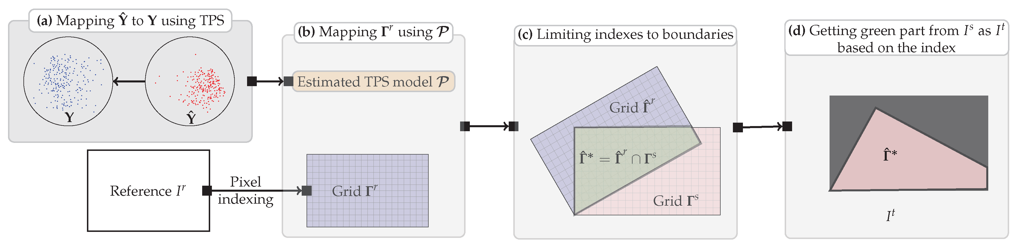
2.5. Image Transformation and Resampling

Once we have the transformed sensed feature point set $\widehat{\mathbf{Y}}$, a mapping function can be constructed based on the corresponding set, i.e., $\mathcal{I}={\{{\mathbf{y}}_i,{\widehat{\mathbf{y}}}_i\}}_{i=1}^m$ and thus to register the images. There are two choices. (i) Forward approach: directly transforming the sensed image $I^s$ using the mapping function. (ii) Backward approach: determining the transformed image $I^t$ from $I^s$ using the grid of the reference image $I^r$ and the inverse of the mapping. Since (i) is complicated to implement, as it can produce holes and/or overlaps in the output image due to the discretization and rounding, we use the backward approach for image transformation, and the flowchart is shown in Figure 6.

Let $\widehat{\mathbf{Y}}$ be the source, $\mathbf{Y}$ the target, the TPS kernel is defined as $\mathcal{K}({\widehat{\mathbf{y}}}_i,{\widehat{\mathbf{y}}}_j)=\parallel {\widehat{\mathbf{y}}}_i-{\widehat{\mathbf{y}}}_j{\parallel }^{2}log\parallel {\widehat{\mathbf{y}}}_i-{\widehat{\mathbf{y}}}_j\parallel$, thus, the TPS transformation model is obtained by

$$\mathcal{P}={\left(\begin{array}{cc}\mathcal{K}& \mathbf{Q}\\ {\mathbf{Q}}^T& \mathbf{O}\end{array}\right)}^{-1}\left(\begin{array}{c}\mathbf{Y}\\ \mathbf{0}\\ \mathbf{0}\\ \mathbf{0}\end{array}\right)$$

(16)

where the TPS model $\mathcal{P}$ is of size $(m+3)\times 3$, $\mathbf{O}$ is a $3\times 3$ matrix of zeros and $\mathbf{Q}$ is the $m\times 3$ matrix with the $i^{th}$ row denotes $(1,{\widehat{\mathbf{y}}}_{ia},{\widehat{\mathbf{y}}}_{ib})$, where ${\widehat{\mathbf{y}}}_{ia}$ and ${\widehat{\mathbf{y}}}_{ib}$ indicate the coordinates of ${\widehat{\mathbf{y}}}_i$.

A regular grid ${\mathbf{\Gamma }}_{Z\times 2}^r={\{{\gamma }_1^r,{\gamma }_2^r,...{\gamma }_Z^r\}}^T$ is obtained by a pixel-by-pixel indexing process on the reference image $I^r$, where $Z=N_w^{\prime }\times N_h^{\prime }$. Let grid ${\mathbf{\Gamma }}^r$ be the source point set, $\mathcal{P}$ the TPS transformation model, the transformed grid is obtained by first computing

$${\widehat{\mathbf{\Gamma }}}_{Z\times 3}^{\mathbf{r}}=\left(\begin{array}{cc}{\mathcal{K}}^{\prime }& {\mathbf{Q}}^{\prime }\end{array}\right)\mathcal{P},$$

(17)

then restoring the dimension of the grid to 2 by ${\widehat{\mathbf{\Gamma }}}^{\mathbf{r}}\leftarrow \left(\begin{array}{cc}{\widehat{\mathbf{\Gamma }}}_{(·,1)}^{\mathbf{r}}& {\widehat{\mathbf{\Gamma }}}_{(·,2)}^{\mathbf{r}}\end{array}\right)$, where the $Z\times m$ kernel ${\mathcal{K}}^{\prime }=\parallel {\gamma }_i^r-{\widehat{\mathbf{y}}}_j{\parallel }^{2}log\parallel {\gamma }_i^r-{\widehat{\mathbf{y}}}_j\parallel$, ${\mathbf{Q}}^{\prime }$ is the $Z\times 3$ matrix with the $i^{th}$ row denotes $(1,{({\gamma }_i^r)}_a,{({\gamma }_i^r)}_b)$ and ${\widehat{\mathbf{\Gamma }}}_{(·,i)}^{\mathbf{r}}$ denotes the $i^{th}$ column of ${\widehat{\mathbf{\Gamma }}}^{\mathbf{r}}$. Let ${\mathbf{\Gamma }}^{\mathbf{s}}$ be the grid obtained on $I^s$, we have

$${\widehat{\mathbf{\Gamma }}}^{*}={\widehat{\mathbf{\Gamma }}}^{\mathbf{r}}\cap {\mathbf{\Gamma }}^{\mathbf{s}}.$$

(18)

Finally, the transformed image $I^t$ is obtained by getting intensities from the sensed image $I^s$ based on ${\widehat{\mathbf{\Gamma }}}^{*}$, and setting the rest of pixels to black. Note that the bicubic interpolation is used to improve the smoothness of $I^t$, to be more precisely, the intensities of each pixel in $I^t$ is determined by summing the weighted neighbor pixel intensities within a $4\times 4$ window.

2.6. Method Analysis

Figure 7 demonstrates the advantage of the MGMM by comparing against the single feature based method, e.g., CPD. At the first iteration, we can see that the initial estimated coordinates by CPD are the regional center of masses, while they are close to the real target coordinates using our method. This helps us recover a good initial pose for aligning the two point sets. Iterating CPD even more, the estimated coordinates are still regional center of masses, and a much better source coordinates obtained by our method. Finally, our method outperforms with less iterations. The obvious difference within red rectangles results from that the estimating ranges i.e., covariances ${\sigma }^2$ of the GMMs in CPD wane to too small a magnitude whereas the distance between points are relatively large. The meaningless probabilities ${\mathbf{P}}^{*}$ provide a bad ${\mathbf{X}}^{*}$, which can not lead $\mathcal{T}\left(\mathbf{Y}\right)$ anymore. Moreover, we see that many green circles are missing from the red rectangle in CPD, and collapsed to $(0,0)$, in the contrary, all the green circles correctly distribute to where they should be, yet only the outliers have no circles in our method.

To examine by which the reliability of our method is mainly contributed, we also additionally compare the accuracy of the feature point sets registration using our method against GMMREG [36], which considers the registration problem as one of the aligning two Gaussian mixture models, and estimates the transformation by minimizing the $L_2$ distance between the two models. As shown in Figure 8, though the $L_{2}E$ estimator is employed, there exists obvious deviations in the result of GMMREG, while our method shows feasible performance. This implies that the accuracy of correspondence and transformation is mainly improved by the strategy based on the complementation and combination of multiple image features using the MGMM.

2.6.1. Computational Complexity

The local geometric feature discrepancy is measured by using the SC, it takes $\mathcal{O}\left(m\right)$ time to build the SC for one point, which therefore takes $\mathcal{O}\left(m^2\right)$ time to build for m points. Note that the Hungarian algorithm which is used to solve the problem of bipartite graph matching with worst-cost time $\mathcal{O}\left(m^3\right)$ is not included in our method. The Matlab Optimization toolbox, e.g., the Matlab function fminunc, which implicitly uses the BFGS Quasi-Newton method with a mixed quadratic and cubic line search procedure,. is used for solving the numerical optimization method, and the total complexity is approximately $\mathcal{O}(m^3+2m^2)$. Overall, the time complexity of our method is $\mathcal{O}\left(m^3\right)$. For storing kernel $\mathbf{\Theta }$, the space complexity of our method is $\mathcal{O}\left(m^2\right)$.

2.6.2. Parametric Setting

The default threshold $1.5$ is used to extract the putative corresponding set ${\{{\mathbf{x}}_i,{\mathbf{y}}_i\}}_{i=1}^n$ as well as the SIFT descriptors ${\{{\mathbf{u}}_i,{\mathbf{v}}_i\}}_{i=1}^n$. The bins of the SC is set to default, i.e., $B=12\times 5$. The constant $\alpha$ controls the trade-off between the global and local geometric feature discrepancy. The constant $\zeta$ weights the uniform distribution $\frac{1}{n}$ for outlier dealing. The two annealing schemes, i.e., gradually update ${\sigma }^2\leftarrow ϵ{\sigma }^2$ and ${\rho }^2\leftarrow \kappa {\rho }^2$, which deal with the non-convexity play important role in our method. A slow annealing, e.g., close to 1, is always preferred without the consideration of the efficiency issue. The constant $t^{\sigma }$ and $t^{\rho }$ determine the maximum iteration numbers of our method and the function fminunc in Matlab. $\beta$ determines the neighborhood size of the source point set. $\lambda$ controls the influence of the geometric constraint on the transformation $\mathcal{T}$. We set $\alpha =10$, $\zeta =0.3$, $ϵ=0.9$, $\kappa =0.75$, $\beta =2$ and $\lambda =3$, and initializing ${\sigma }^2$ and ${\rho }^2$ to 1 and $0.05$, respectively. Due to the iterations need termination conditions, we use the function fminunc in Matlab with the options: $\{MaxIter=50\}$, namely $t^{\rho }=50$, and set $t^{\sigma }=100$.

3. Experiments and Results

SIFT [11], SURF [13], CPD [25], GLMDTPS [30], RSOC [21], totally five state-of-the-art methods are compared against our method in the experiments. These methods can mainly categorize into three types based on the methods of feature extraction. Type 1: using open source $VLFeat$ toolbox with default threshold $1.5$, i.e., SIFT, CPD, GLMDTPS and ours. Type 2: using open source VLFeat toolbox with specific built-in setting, i.e., RSOC. Type 3: using Matlab open source $OpenSURF$ function with default setting, i.e., SURF. Since both the feature matching and image registration are considered in our method, we fairly design three series of experiments. (I) Due to the employment of the same feature point sets, quantitative comparison on feature matching is carried out on methods of Type 1 using the precision ratio (PR). However, since no inlier set is outputted from GLMDTPS, the compared methods are SIFT, CPD and ours. (II) Quantitative comparison and Qualitative demonstration on image registration are carried out on all the methods using the root of mean square error (RMSE), mean absolute error (MAE) and standard deviation (SD). (III) By using the different datasets, quantitative and qualitative demonstration on feature matching and image registration are carried out to examine the availability and robustness of our method using the PR, RMSE, MAE and SD. Three datasets are used which are: (i) 100 pairs of UAV images with horizontal viewpoint changes; (ii) 150 pairs of UAV images pairs with vertical viewpoint changes; and (iii) 50 pairs of satellite images registration with horizontal and vertical viewpoint changes. The experimental design is shown in

Table 1. The experimental design.

Series	Criteria	Compared Methods	Datasets Used
I	PR	SIFT, CPD, Ours	(i), (ii)
II	All	All	(i), (ii)
III	All	Ours	(iii)

. All experiments are tested on a PC with 2.20 GHz Intel CPU and 8 GB memory.

Generally, the downsampled image size is selected based on the performance and accuracy requirements of the underlying system. High sampling rates might lead to more locally accurate at the cost of the far more time-consuming, whereas the globality is our main concern. Therefore, a procedure of downsample, which is based on the bicubic interpolation using Matlab $imresize$ function, is carried out on all image pairs. The downsampled images have a resolution in the range from $640\times 450$ to $1100\times 850$ pixels, thus the more compact feature points can therefore be extracted. The number of the extracted feature points for Type I to III methods are shown in

Table 2. Numbers of the extracted feature points.

Type 1	Type 2	Type 3
87 to 505	30	35 to 165

.

3.1. Evaluation Criterion

$$Precision=\frac{TP}{TP+FP},$$

(19)

where $TP$ denotes true positive, $FP$ denotes false positive, $0\le Precision\le 1$. To obtain the estimated inlier set $\mathcal{I}$, different approaches are used based on the characteristic of each method. For SIFT, it is just an array from 1 to n; for CPD and our method, it is obtained by:

$$\mathcal{I}=\{i:{\left({\mathbf{P}}^T\mathbf{1}\right)}_i>\varrho \},$$

(20)

where the threshold is set to $\varrho =0.75$ empirically.

The RMSE, MAE and SD are used to quantify the registration accuracy. We manually determine at least 10 pairs of landmarks between the sensed image and the reference image as ground-truth, and all the landmarks are well-distributed and selected on the easily identified places around the interest areas. The related formulations and the definitions in statistics are as follows:

$$RMSE=\sqrt{\frac{1}{m^{\prime }}{\displaystyle \sum _{i=1}^{m^{\prime }}}({\mathbf{y}}_i^t-{\mathbf{x}}_i^t)},$$

(21)

The root mean square error is a frequently used measure of the distance between selected landmark and its corresponding point actually located, where $m^{\prime }$ is the total number of the selected landmark, and ${\mathbf{y}}_i^t$ is the landmark that corresponds to ${\mathbf{x}}_i^t$;

$$MAE=\frac{{\displaystyle \sum _{i=1}^{m^{\prime }}}|{\mathbf{y}}_i^t-{\mathbf{x}}_i^t|}{m^{\prime }};$$

(22)

the mean absolute error is a quantity used to measure how close the landmark are to its corresponding point;

$$SD=\sqrt{\frac{1}{m^{\prime }}\sum _{i=1}^{m^{\prime }}{\left[d({\mathbf{x}}_i^t,{\mathbf{y}}_i^t)-RMSE\right]}^2},$$

(23)

the standard deviation informally measures how far the distance of a landmark pair are spread out from its RMSE, where $d(·,·)$ denotes the distance.

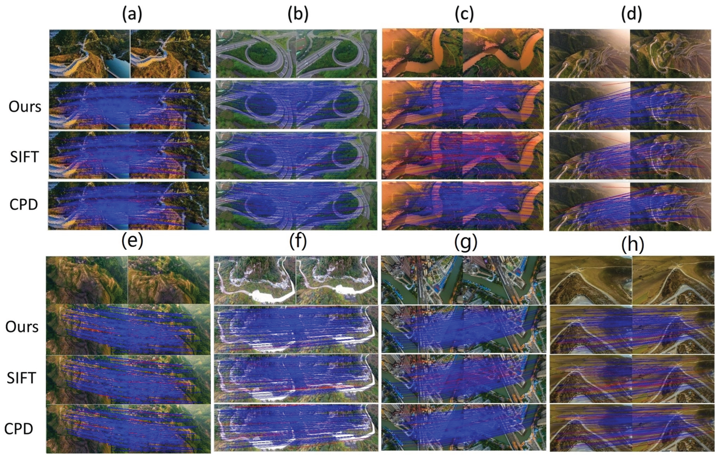
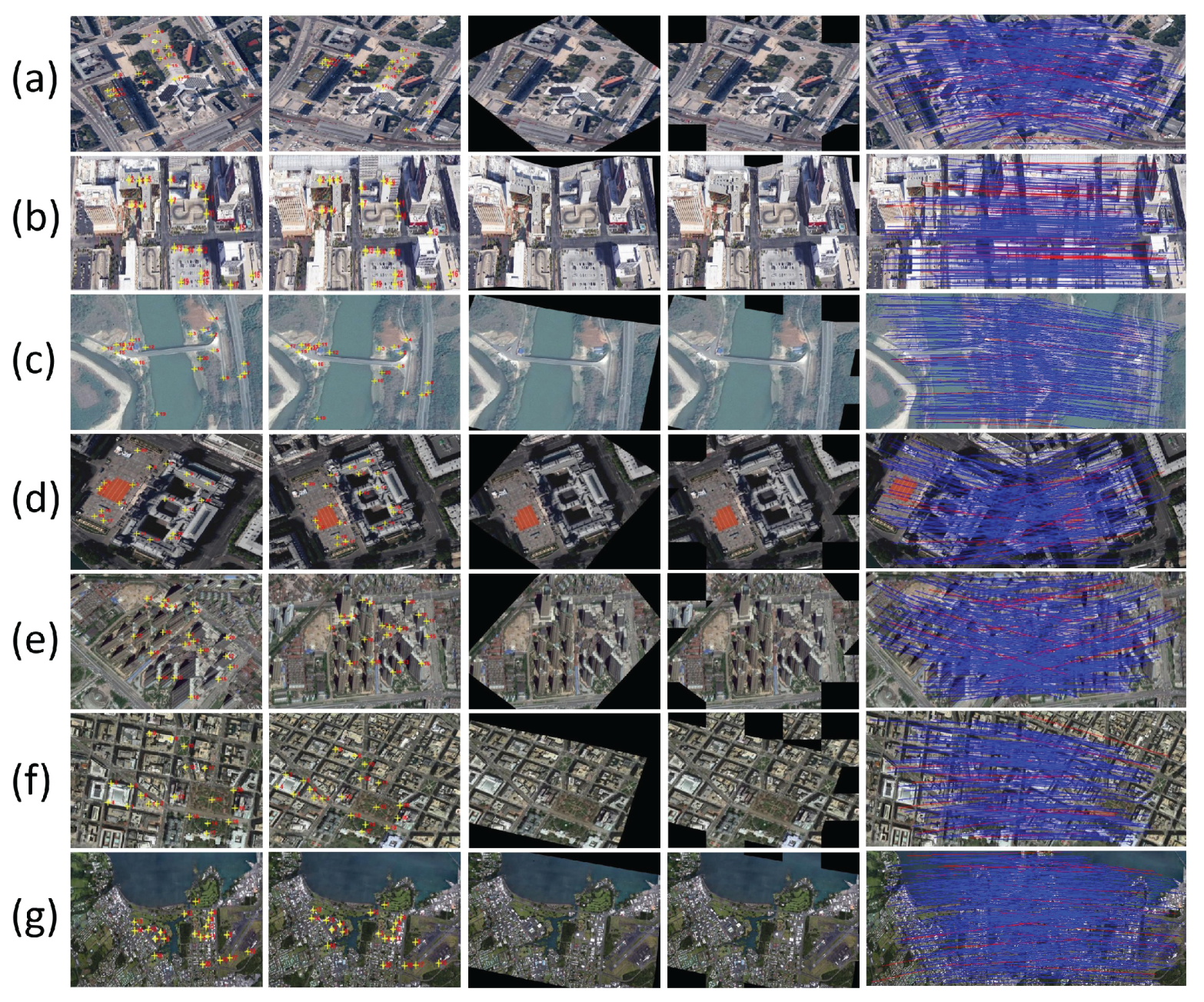
3.2. Results on Feature Matching

The quantitative results are shown in

Table 3. Experimental results of series (I). Quantitative comparisons on the mean PR of Type I method are carried out. Bold fonts indicate the best results. All Units are in percentage.

Dataset	SIFT	CPD	Ours
(i)	78.30	90.81	98.25
(ii)	72.78	90.17	97.15

. Feature matching results on eight typical image pairs are demonstrated in Figure 9, as well as the quantitative results of the eight selected image pairs.

The extraction of the SIFT feature point sets is based on the intensity information, or, to be more precisely, the scale-space extrema. However, for all the data which contain viewpoint changes, the objects captured in one image may be missing or distorted non-rigidly from another image, which further lead to false matching. Based upon the SIFT putative corresponding set, CPD estimates the correspondence using Euclidean distance, a single global geometric structure discrepancy for correspondence estimation. The motion coherent based geometric constraint is employed to regularize the displacement field between the point sets. However, as we mentioned before, the regular Gaussian mixture model is incapable of dealing with mixture features, and for Euclidean distance, $p\left({\mathbf{x}}_a\right|{\mathbf{y}}_j)=p\left({\mathbf{x}}_b\right|{\mathbf{y}}_j)$ if $\parallel {\mathbf{x}}_a-{\mathbf{y}}_j{\parallel }^2={\parallel {\mathbf{x}}_b-{\mathbf{y}}_j\parallel }^2$ even when the neighborhood structure of ${\mathbf{x}}_a$ and ${\mathbf{x}}_b$ are totally different. In our method, both the intensity information and the global and local geometric structure discrepancies are considered, the complementation and combination of these features provide a reliable correspondence estimation. We summarize the key components employed in these three method as: (I) intensity information discrepancy; (II/III) global/local geometric structure discrepancy; (IV) geometric constraint. Thus, SIFT use only (I), CPD employs (II) and (IV), and our method adopts both. Therefore, the result shows a increasing tendency on PR from left to right.

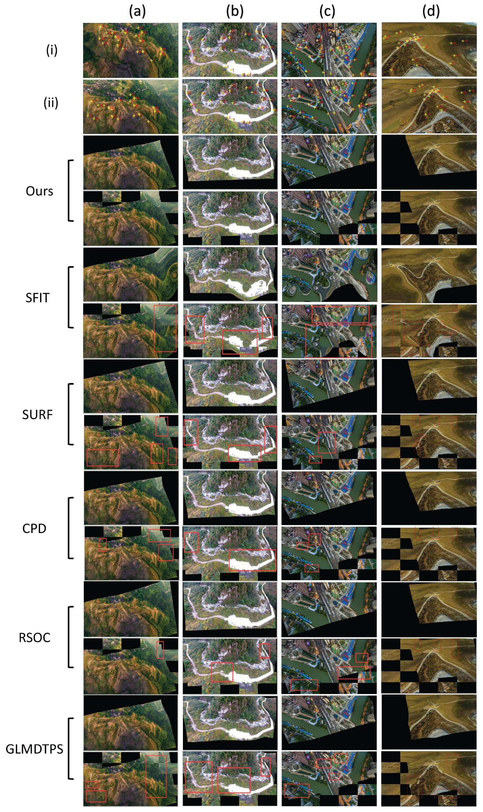
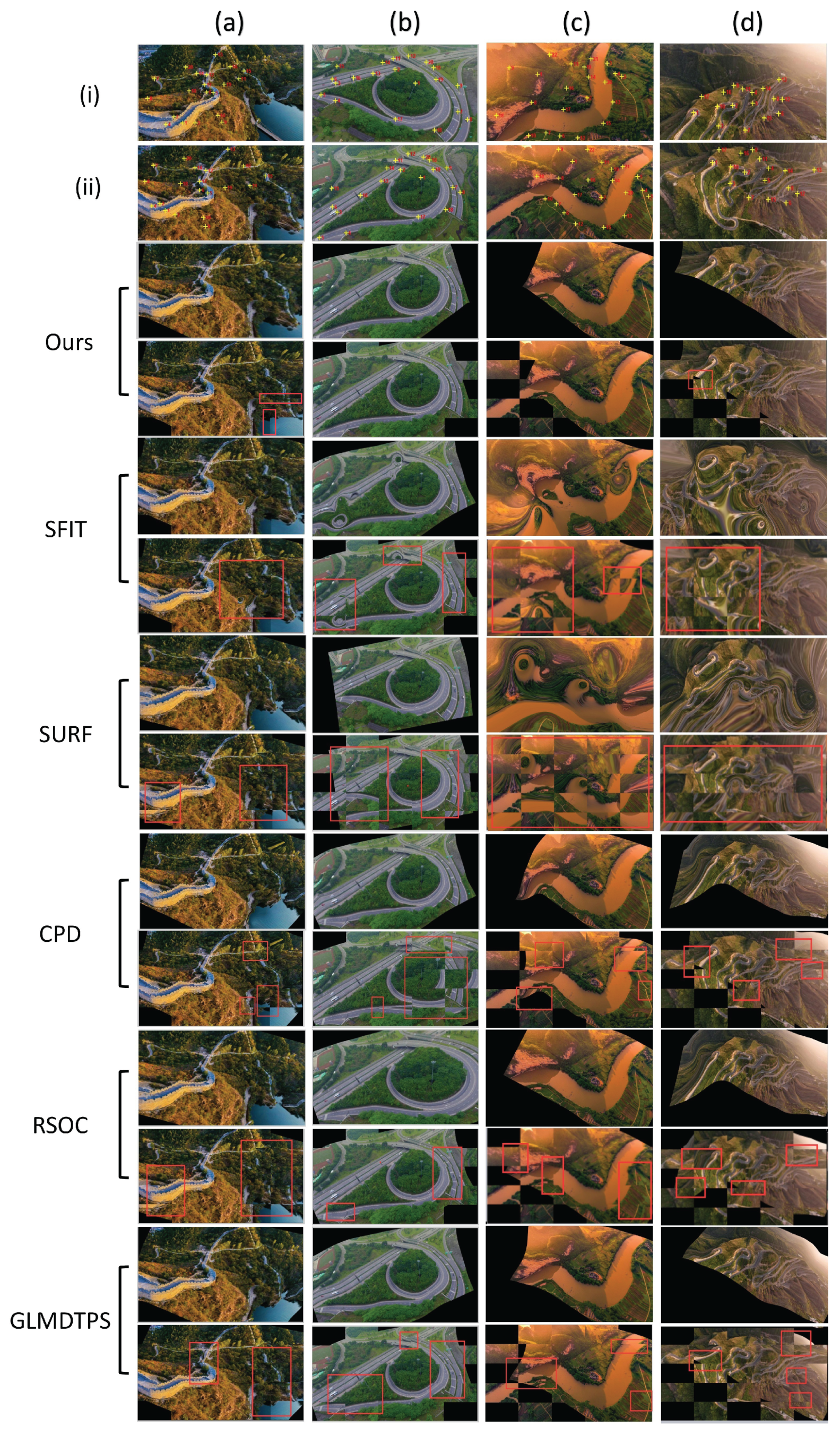
3.3. Results on Image Registration

Quantitative comparison using the mean RMSE, MAE and SD are shown in

Table 4. Experimental results on series (II). Quantitative comparisons on image registration measured using the mean RMSE, MAE and SD are carried out. Bold fonts indicate the best results. All units are in pixel.

	Dataset	SIFT	SURF	CPD	GLMDTPS	RSOC	OURS
RMSE	(i)	13.5287	7.9837	3.2386	3.0152	2.2737	1.0171
	(ii)	11.4466	7.0627	7.2645	5.5991	4.1743	1.4331
MAE	(i)	16.0080	12.2803	7.5404	7.1459	6.4448	4.0271
	(ii)	14.2989	9.8411	10.3778	9.1102	7.3585	3.9188
SD	(i)	14.1826	10.2241	5.8594	5.4353	4.8013	3.1957
	(ii)	11.9613	8.2523	4.3619	7.6531	5.7844	3.0021

. The transformed images and $5\times 5$ checkboards on eight typical image registration examples from dataset (i) and (ii) are shown (four examples per dataset) in Figure 10 and Figure 11, respectively.

A low computation complexity is one of the advantages for registering image based on the extracted feature points. However, its registration accuracy might be poor which in general cannot obtain accurate dense correspondences. Therefore, the number of the extracted feature points plays a crucial role to alleviate this problem. In this experiment, SURF and RSOC, which extract relative small number of feature points, are sensitive to false matches. Since RSOC employs robust graph matching technique to remove dubious matches, its performance remains relative high. By contrast, the result shows that directly yielding the transformed images by the putative corresponding set of SIFT with a default threshold is not a good idea when viewpoint changes exist. Fewer and more reliable feature points can generate by setting a high threshold, which in turn limits the registration accuracy based on more sparse correspondences. GLMDTPS employs mixture features as well. The global feature is the pairwise Euclidean distance, and the local feature first respectively generates two index matrices of K nearest neighbors for two point sets. After translating the two currently computing points together, the local distance is obtained by summing the squared Euclidean distance between the $i^{th}$ neighbors. The defect of the employed features is that it is sensitive to outliers and similar neighborhood structure. Unlike the contour point set, the feature point set extracted in remote sensing images distributes irregularly, the local distance employed by GLMDTPS is therefore ambiguous, resulting in more dubious estimation in local area.

3.4. Reliability and Availability Examination of Our Method

In this series of experiment, we examine the reliability and availability of our method using Satellite Image with Horizontal and Vertical Viewpoint Changes. The PR, RMSE, MAE and SD are shown in

Table 5. Experimental results on series (III). Quantitative tests on feature matching and image registration are carried out to examine the availability and robustness of our method using the PR, RMSE, MAE and SD. (a) to (g): results on the corresponding pairs of Figure 12. Mean: the mean of results on all image pairs of dataset (iii). For the PR, the units are in percentage, for the RMSE, MAE and SD, the units are in pixel.

	(a)	(b)	(c)	(d)	(e)	(f)	(g)	Mean
$PR$	96.88	96.77	95.97	95.77	95.09	98.19	95.57	96.54
$RMSE$	0.8358	1.3963	1.9556	1.4272	0.7743	1.4342	0.3171	1.1628
$MAE$	2.1458	4.0208	2.9097	1.9317	2.5778	2.3542	2.2958	2.6051
$SD$	1.8562	2.5498	2.5171	1.8061	2.1429	2.0098	2.0717	2.1362

, seven typical images are selected to show the image registration results in Figure 12. We see that our method maintains accurate alignments in all experiments. Which means that our proposed method can successfully handle the satellite image registration problem in most time.

4. Conclusions

In this paper, we proposed an accurate method for remote sensing image registration with different viewpoint. The main contributions of this paper are considered as follows. (i) The MGMM is constructed for simultaneously dealing with different types of image features. (ii) Two types of features are using to form a feature complementation, i.e., the Euclidean distance and shape context to measure the global and local geometric structure discrepancies, and the SIFT distance which is endowed with the intensity information are combined and substituted into the MGMM by which the reliable correspondence is obtained. (iii) To prevent the ill-posed problem, a geometric constraint term based on coherent velocity field is introduced into the L2E-based energy function and achieves accurate transformation updating. Experiments on three series of remote sensing images obtained from the unmanned aerial vehicle (UAV) and Google Earth with different viewpoint demonstrate that our method shows best registration performances against five state-of-the-art methods.

References

1. Zitov, B.; Flusser, J. Image registration methods: A survey. Image Vis. Comput. 2003, 21, 977–1000. [Google Scholar] [CrossRef]
2. Brown, L. A survey of image registration techniques. ACM Comput. Surv. 1992, 41, 325–376. [Google Scholar] [CrossRef]
3. Maintz, J.; Viergever, M. A survey of medical image registration. Med. Image Anal. 1998, 2, 1–36. [Google Scholar] [CrossRef]
4. Wang, X.; Li, Y.; Wei, H.; Liu, F. An asift-based local registration method for satellite imagery. Remote Sens. 2015, 7, 7044–7061. [Google Scholar] [CrossRef]
5. Liu, S.; Tong, X.; Chen, J.; Liu, X.; Sun, W.; Xie, H.; Chen, P.; Jin, Y.; Ye, Z. A Linear Feature-Based Approach for the Registration of Unmanned Aerial Vehicle Remotely-Sensed Images and Airborne LiDAR Data. Remote Sens. 2016, 8, 82. [Google Scholar] [CrossRef]
6. Sedaghat, A.; Mokhtarzade, M.; Ebadi, H. Uniform Robust Scale-Invariant Feature Matching for Optical Remote Sensing Images. IEEE Trans. Geosci. Remote Sens. 2011, 49, 4516–4527. [Google Scholar] [CrossRef]
7. Jensen, J. Introductory Digital Image Processing; Prentice Hall: Upper Saddle River, NJ, USA, 2004. [Google Scholar]
8. Mikolajczyk, K.; Chmid, C. A performance evaluation of local descriptors. In Proceedings of the 2003 IEEE Computer Society Conference on Computer Vision and Pattern Recognition, Madison, WI, USA, 18–20 June 2003; Volume 2. [Google Scholar]
9. Fan, B.; Wu, F.; Hu, Z. Rotationally Invariant Descriptors Using Intensity Order Pooling. IEEE Trans. Pattern Anal. Mach. Intell. 2011, 34, 2031–2045. [Google Scholar] [CrossRef] [PubMed]
10. Harris, C. A combined corner and edge detector. In Proceedings of the 4th Alvey Vision Conference, Manchester, UK, 31 August–2 September 1988; Volume 1988, pp. 147–151. [Google Scholar]
11. Lowe, D. Object recognition from local scale-invariant features. In Proceedings of the IEEE Seventh IEEE International Conference on Computer Vision, Kerkyra, Greece, 20–27 September 1999; Volume 2, p. 1150. [Google Scholar]
12. Lowe, D. Distinctive Image Features from Scale-Invariant Keypoints. Int. J. Comput. Vis. 2004, 21, 91–110. [Google Scholar] [CrossRef]
13. Bay, H.; Ess, A.; Tuytelaars, T.; Van Gool, L. Speeded-Up Robust Features (SURF). Comput. Vis. Image Underst. 2008, 110, 346–359. [Google Scholar] [CrossRef]
14. Li, Q.; Wang, G.; Liu, J.; Chen, S. Robust Scale-Invariant Feature Matching for Remote Sensing Image Registration. IEEE Geosci. Remote Sens. Lett. 2009, 6, 287–291. [Google Scholar]
15. Ke, Y.; Sukthankar, R. PCA-SIFT: A more distinctive representation for local image descriptors. In Proceedings of the 2004 IEEE Computer Society Conference on Computer Vision and Pattern Recognition, 2004. CVPR 2004, Washington, DC, USA, 27 June–2 July 2004; Volume 2, pp. 506–513. [Google Scholar]
16. Dellinger, F.; Delon, J.; Gousseau, Y.; Michel, J. SAR-SIFT: A SIFT-Like Algorithm for SAR Images. IEEE Trans. Geosci. Remote Sens. 2015, 53, 453–466. [Google Scholar] [CrossRef]
17. Sedaghat, A.; Ebadi, H. Remote Sensing Image Matching Based on Adaptive Binning SIFT Descriptor. IEEE Trans. Geosci. Remote Sens. 2015, 53, 5283–5293. [Google Scholar] [CrossRef]
18. Liu, F.; Bi, F.; Chen, L.; Shi, H. Feature-Area Optimization: A Novel SAR Image Registration Method. IEEE Geosci. Remote Sens. Lett. 2016, 13, 242–246. [Google Scholar] [CrossRef]
19. Goncalves, H.; Corte-Real, L.; Goncalves, J. Automatic Image Registration Through Image Segmentation and SIFT. IEEE Trans. Geosci. Remote Sens. 2011, 49, 2589–2600. [Google Scholar] [CrossRef]
20. Gong, M.; Zhao, S.; Jiao, L.; Tian, D. A Novel Coarse-to-Fine Scheme for Automatic Image Registration Based on SIFT and Mutual Information. IEEE Trans. Geosci. Remote Sens. 2014, 52, 4328–4338. [Google Scholar] [CrossRef]
21. Liu, Z.; An, J.; Jing, Y. A simple and robust feature point matching algorithm based on restricted spatial or derconstraints for aerial image registration. IEEE Trans. Geosci. Remote Sens. 2012, 50, 514–527. [Google Scholar] [CrossRef]
22. Ma, J.; Zhao, J.; Tian, J.; Bai, X.; Tu, Z. Regularized vector field learning with sparse approximation for mismatch removal. Pattern Recognit. 2013, 46, 3519–3532. [Google Scholar] [CrossRef]
23. Ma, J.; Zhao, J.; Tian, J.; Yuille, A.; Tu, Z. Robust point matching via vector field consensus. IEEE Trans. Image Proc. 2014, 23, 1706–1721. [Google Scholar]
24. Fischler, M.; Bolles, R. Random Sample Consensus: A Paradigm for Model Fitting with Applications to Image Analysis and Automated Cartography. Commun. ACM 1980, 24, 381–395. [Google Scholar] [CrossRef]
25. Myronenko, A.; Song, X. Point set registration: coherent point drift. IEEE Trans. Pattern Anal. Mach. Intell. 2009, 32, 2262–2275. [Google Scholar] [CrossRef] [PubMed]
26. Liu, H.; Yan, S. Common visual pattern discovery via spatially coherent correspondences. In Proceedings of the IEEE Conference on Computer Vision and Pattern Recognit, San Francisco, CA, USA, 13–18 June 2010; pp. 1609–1616. [Google Scholar]
27. Zhang, Z.; Yang, M.; Zhou, M.; Zeng, X. Simultaneous remote sensing image classification and annotation based on the spatial coherent topic model. In Proceedings of the IGARSS 2014—2014 IEEE International Geoscience and Remote Sensing Symposium, Quebec, QC, Canada, 13–18 July 2014; pp. 1698–1701. [Google Scholar]
28. Ma, J.; Qiu, W.; Zhao, J.; Ma, Y. Robust L2E Estimation of Transformation for Non-Rigid Registration. IEEE Trans. Signal Process. 2015, 63, 1115–1129. [Google Scholar] [CrossRef]
29. Ma, J.; Zhou, H.; Zhao, J.; Gao, Y.; Jiang, J.; Tian, J. Robust Feature Matching for Remote Sensing Image Registration via Locally Linear Transforming. IEEE Trans. Geosci. Remote Sens. 2015, 53, 6469–6481. [Google Scholar] [CrossRef]
30. Yang, Y.; Ong, S.; Foong, K. A robust global and local mixture distance based non-rigid point set registration. Pattern Recognit. 2015, 48, 156–173. [Google Scholar] [CrossRef]
31. Belongie, S.; Malik, J.; Puzicha, J. Shape Matching and Object Recognition Using Shape Contexts. IEEE Trans. Pattern Anal. 2002, 24, 509–522. [Google Scholar] [CrossRef]
32. Kortgen, M.; Park, G.; Novotni, M.; Klein, R. 3D shape matching with shape context. In Proceedings of the 7th Central European Seminar on Computer Graphics, Budmerice, Slovakia, 22–24 April 2003; pp. 22–24. [Google Scholar]
33. Tikhonov, A.N.; Arsenin, V.Y. Solutions of Ill-Posed Problems; Winston & Sons Inc.: Washington, DC, USA, 1977. [Google Scholar]
34. Scott, D. Parametric statistical modeling by minimum integrated sqaure error. Technometrics 2001, 43, 274–285. [Google Scholar] [CrossRef]
35. Yuille, A.; Grzywacz, N. A Mathematical Analysis of the Motion Coherence Theory. Int. J. Comput. Vis. 1989, 3, 155–175. [Google Scholar] [CrossRef]
36. Jian, B.; Vemuri, B. Robust Point Set Registration Using Gaussian Mixture Models. IEEE Trans. Pattern Anal. Mach. Intell. 2011, 33, 1633–1645. [Google Scholar] [CrossRef] [PubMed]
Figure 1. Illustration of the SC. (a) and (b): diagrams of log-polar histogram bins centered at x i and y j used in computing the shape contexts. (c) and (d): each shape context e.g., h i or h j is a log-polar histogram of the coordinates of the rest of the point set measured using the centered point as the origin, where darker denotes larger value.
Remotesensing 09 00581 g001
Figure 2. Illustration of how the SIFT feature descriptor is obtained. (a): Repeatedly convolving initial image with Gaussians to produce the set of scale space images. (b): Subtracting adjacent Gaussian images to produce the difference-of-Gaussian images. (c): Extrema detection by comparing a pixel (marked with red circle) to its 26 neighbors in 3 × 3 regions at the current and adjacent scales (marked with green circles). (d): Feature descriptor creation by computing the gradient magnitude and orientation at each image sample point. a Gaussian window indicated by the overlaid circle is used as weighting. (e) Orientation histograms accumulation by summarizing the contents over 4 × 4 subregions (a 2 × 2 subregions is shown for convenience), with the length of each arrow corresponding to the sum of the gradient magnitudes near that direction within the region, generating 4 × 4 × 8 descriptors, where 8 is the number of directions.
Remotesensing 09 00581 g002
Figure 3. The robustness comparison between L 2 E and M L E . We estimate the mean of a normally distributed sample N ( 0 , 1 ) with contaminations of extra samples N ( 5 , 1 ) . The outlier to the inlier ratios are 5 % , 10 % , 20 % , 30 % and 50 % . The vertical dash lines indicate the extrema. L 2 E has a global minimum at approximately 0 and a local minimum at approximately 5, both of which conform to the inlier and outlier distributions, respectively. However, the deviation of MLE increases as the ratio grows.
Remotesensing 09 00581 g003
Figure 4. Illustration of the velocity field. (a): two given point pairs. (b): a coherent velocity field. (c): a velocity field that is less coherent.
Remotesensing 09 00581 g004
Figure 5. The summary of our method. (a): Extracting putative corresponding set { x i , y i } i = 1 n and SIFT descriptor set { u i , v i } i = 1 n using SIFT algorithm, and obtaining two types of discrepancies, i.e., the global and local geometric structure discrepancies G and L , and intensity information discrepancy S . (b): substituting the combined features into the optimization framework and obtaining the transformed point set Y ^ , note that a loop is included. (c): Image registration based on the backward approach.
Remotesensing 09 00581 g005
Figure 6. Illustration of the image transformation and resampling. (a) Computing a TPS transformation model P which maps Y ^ back onto Y , meanwhile, constructing a grid Γ r which is of the same size as I r ; (b) Mapping Γ r using P , obtaining Γ ^ r ; (c) Limiting indexes to boundaries of Γ ^ r Γ s ; (d) Getting intensities from I s within boundaries to generate I t , each pixel in I t is determined by the bicubic interpolation.
Remotesensing 09 00581 g006
Figure 7. Demonstration of the advantage of the MGMM. Red *: the target feature point set X . Green ∘: the estimated corresponding point set X * . Blue +: the source feature point set T ( Y ) . Upper row and lower row: registration process of CPD and our method. X and Y are extracted from a remote sensing image pair.
Remotesensing 09 00581 g007
Figure 8. Examination of the availability of the MGMM. Red *: the target feature point set X . Blue ∘: the source feature point set T ( Y ) . (a,b) registration result of GMMREG and our method. Obvious deviation exists in the result of GMMREG.
Remotesensing 09 00581 g008
Figure 9. Feature matching demonstrations on eight typical image pairs of dataset (i) and (ii). For each image pair, rows from the first to the fourth are: the image pair, the results on feature matching of ours, SIFT and CPD, respectively. Blue lines indicate true positive and true negative, red lines indicate false positive and false negative. The PRs of three methods on each image pairs are listed from (a) to (h) as follows. Ours: 99.00, 99.29, 97.31, 97.40, 99.32, 99.62, 98.31, 98.89; SIFT: 85.68, 85.18, 45.12, 60.26, 82.43, 80.34, 82.43, 83.55; CPD: 86.86, 88.14, 85.02, 88.24, 87.22, 85.55, 89.76, 85.23.
Remotesensing 09 00581 g009
Figure 10. Registration examples on four typical image pairs from dataset (i). The first two rows: the sensed and reference image, with the yellow crosses denoting the landmarks. Rows from the third to the end are the registration results of ours, SIFT, SURF, CPD, RSOC and GLMDTPS. For each method, the registration results are shown using two rows, with the upper row showing the transformed image, and the lower row showing the 5 × 5 checkboard. The registration errors are highlighted using the red rectangles.
Remotesensing 09 00581 g010
Figure 11. Registration examples on four typical image pairs from dataset (ii). The first two rows: the sensed and reference image, with the yellow crosses denoting the landmarks. Rows from the third to the end are the registration results of ours, SIFT, SURF, CPD, RSOC and GLMDTPS. For each method, the registration results are shown using two rows, with the upper row showing the transformed image, and the lower row showing the 5 × 5 checkboard. The registration errors are highlighted using the red rectangles.
Remotesensing 09 00581 g011
Figure 12. Registration examples on the seven typical satellite image pairs. From (a) to (g) are: Berlin, Las Vegas, Mekong River, Paris, WuHan, Washington and Hawaii. Columns from the left to the right are: the sensed, reference and transformed images, the 5 × 5 checkboards, and the feature matching results. Blue lines indicate true positive and true negative, red lines indicate false positive and false negative.
Remotesensing 09 00581 g012