
Comparison of Satellite Reflectance Algorithms for Estimating Phycocyanin Values and Cyanobacterial Total Biovolume in a Temperate Reservoir Using Coincident Hyperspectral Aircraft Imagery and Dense Coincident Surface Observations

 , ,
, ,  , , ,
, , , 
Abstract
:
1. Introduction
1.1. Background
1.2. Rationale
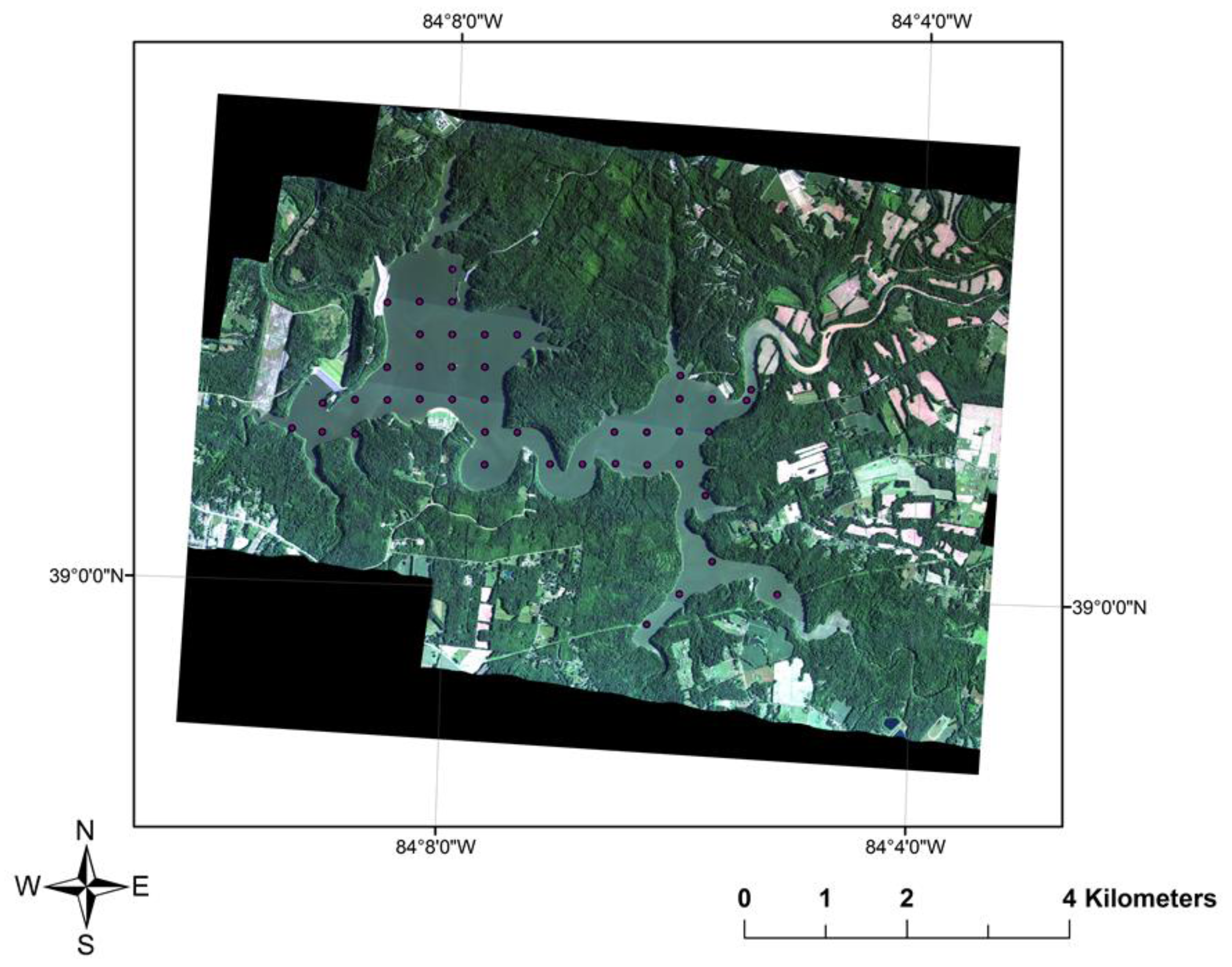
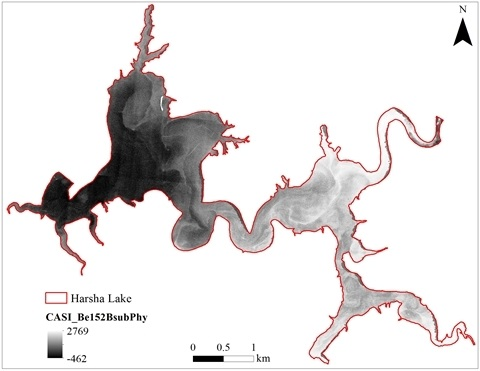
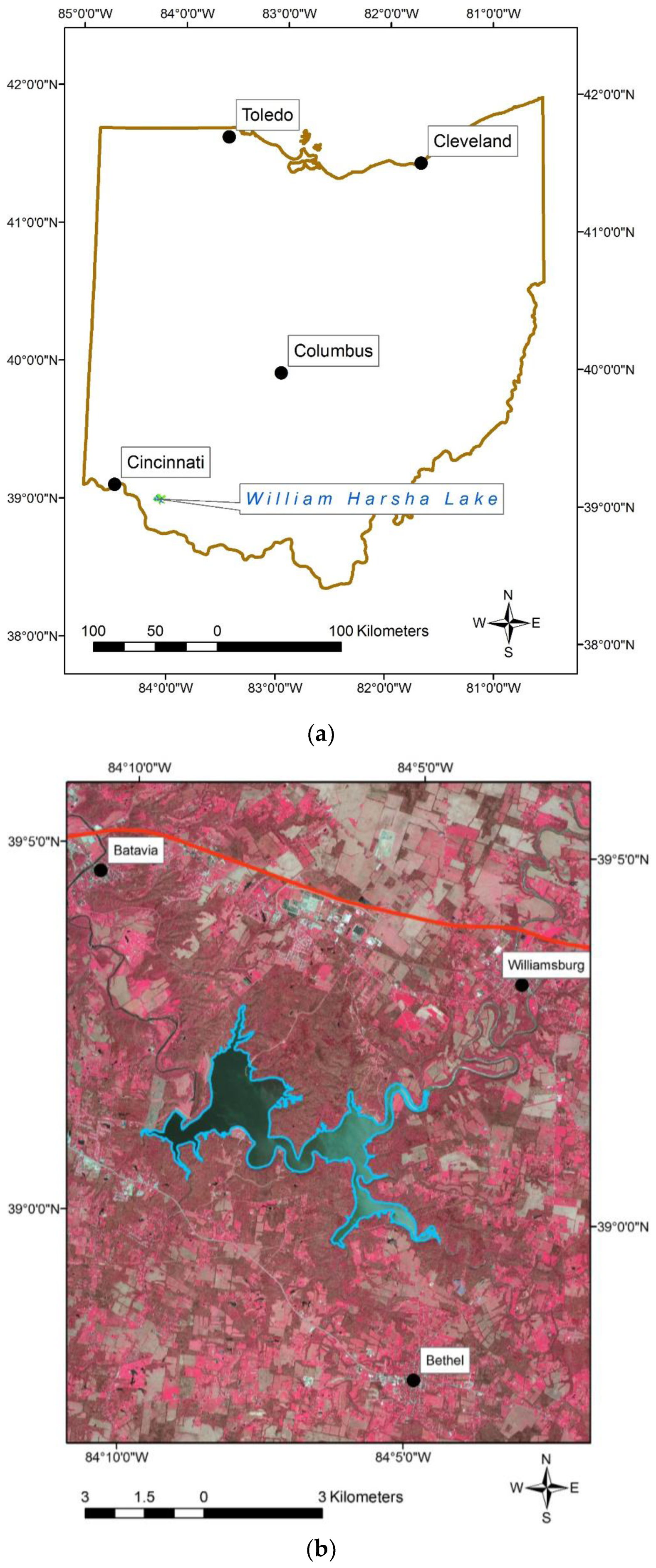
1.3. Study Area
1.4. Approach
2. Methods
2.1. Coincident Surface Observations of BGA
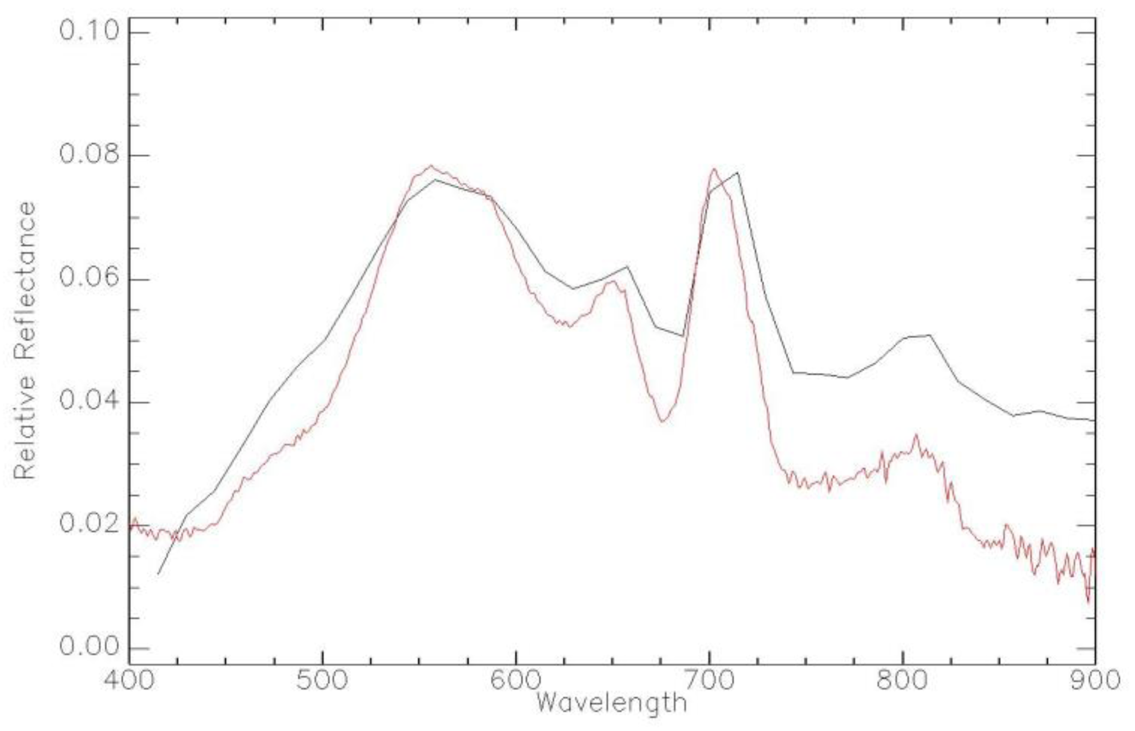
2.2. Atmospheric Correction of CASI Hyperspectral Aircraft Imagery
3. Results
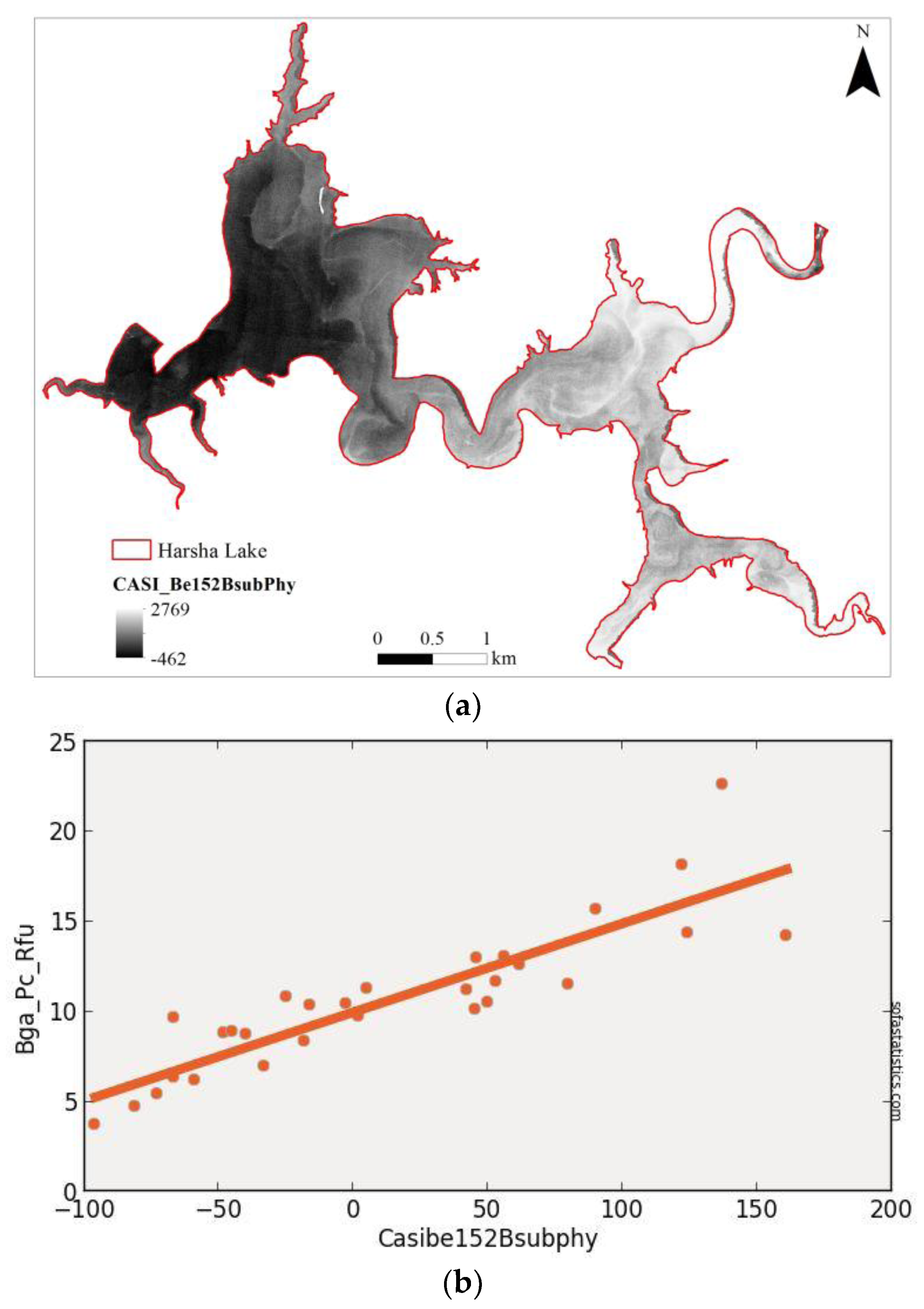
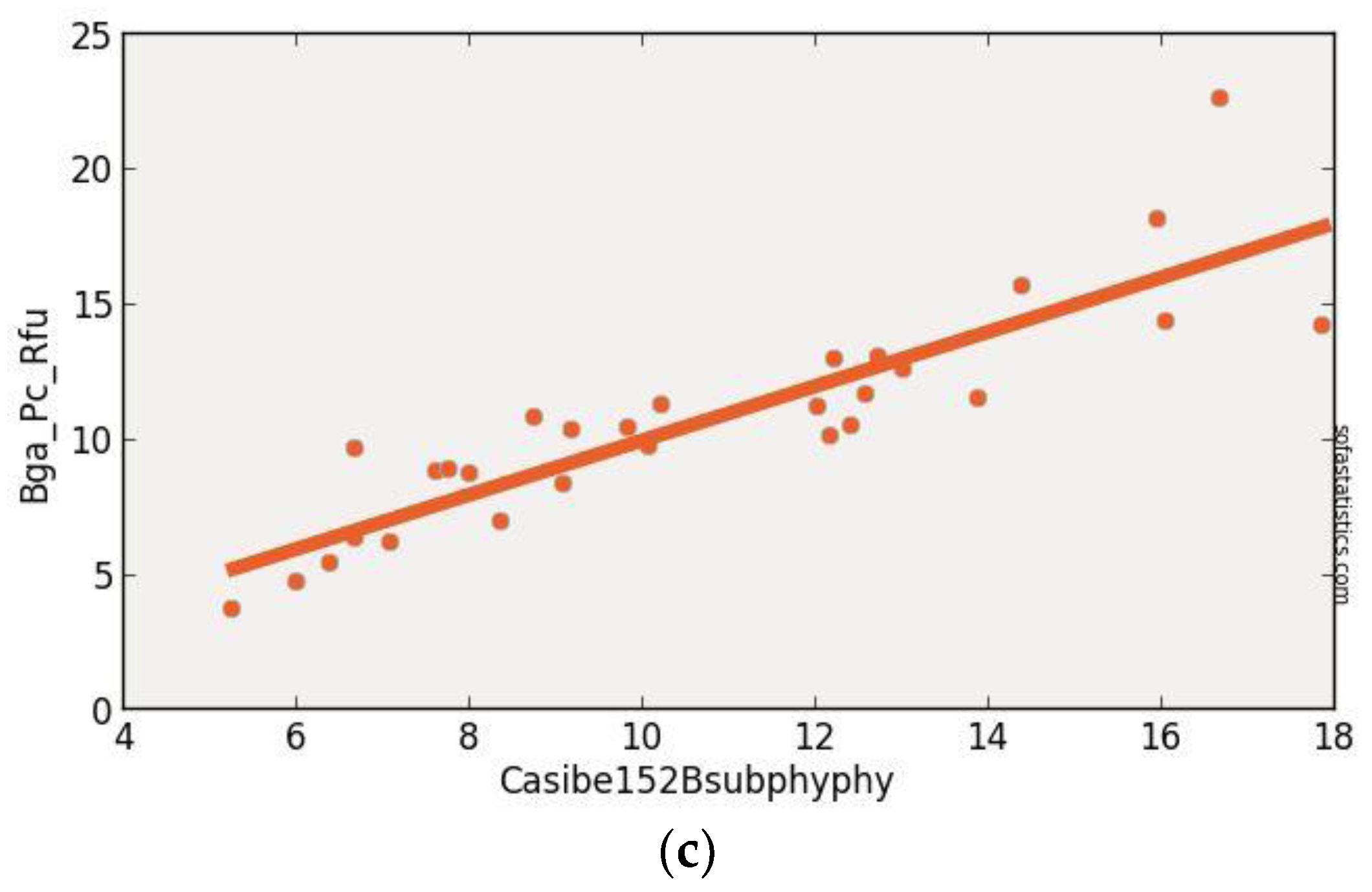
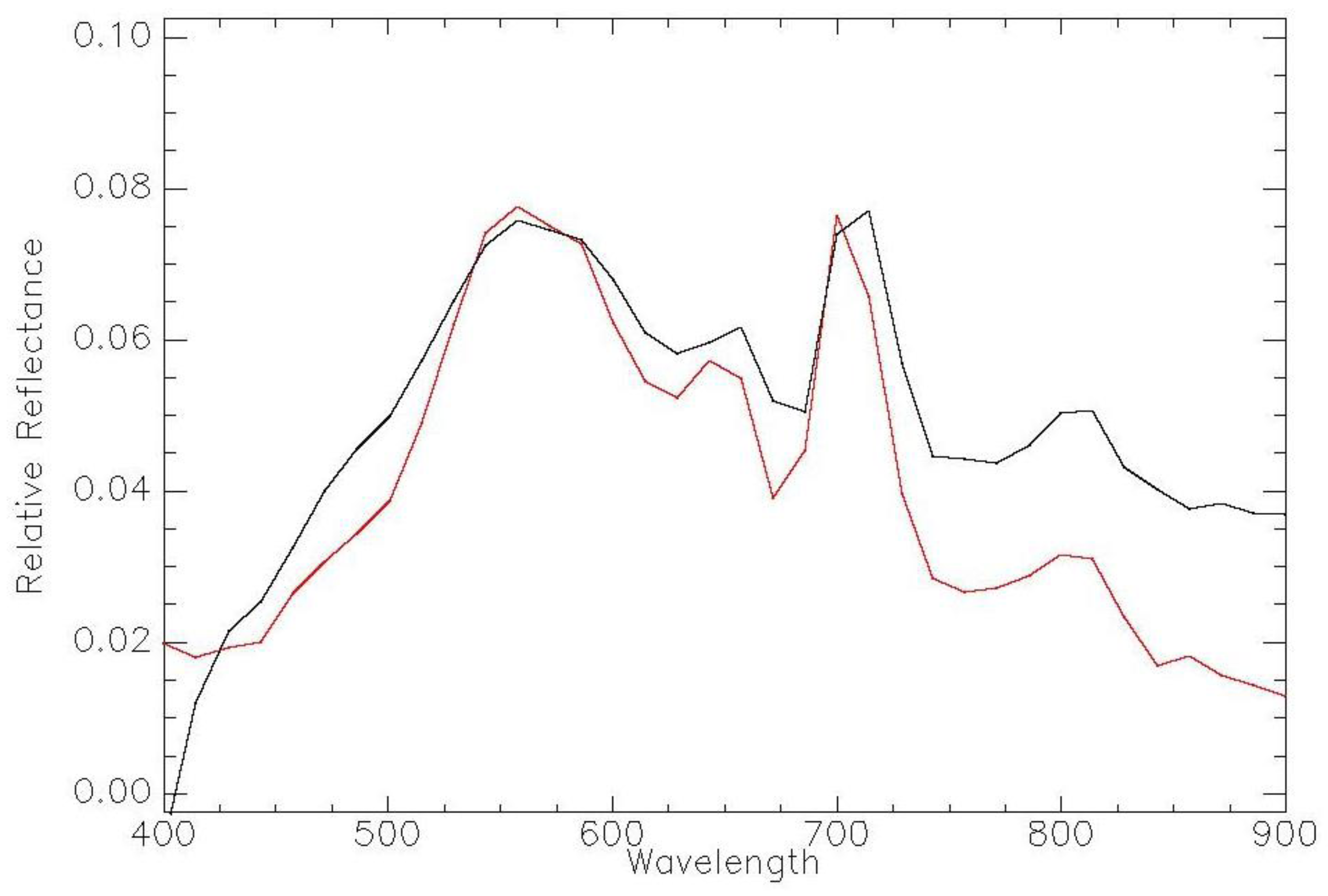
3.1. CASI Imagery
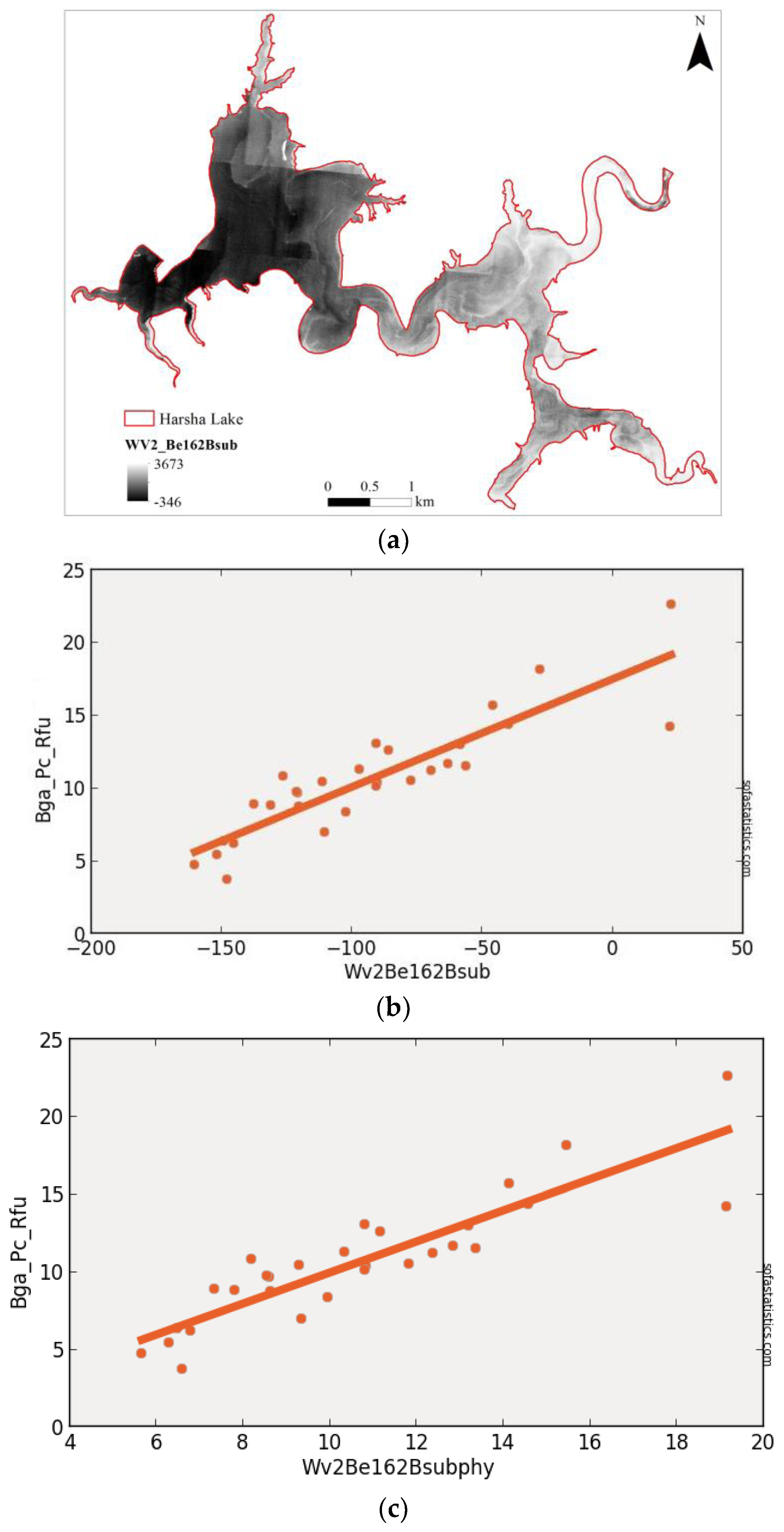
3.2. WorldView-2 (Synthetic)
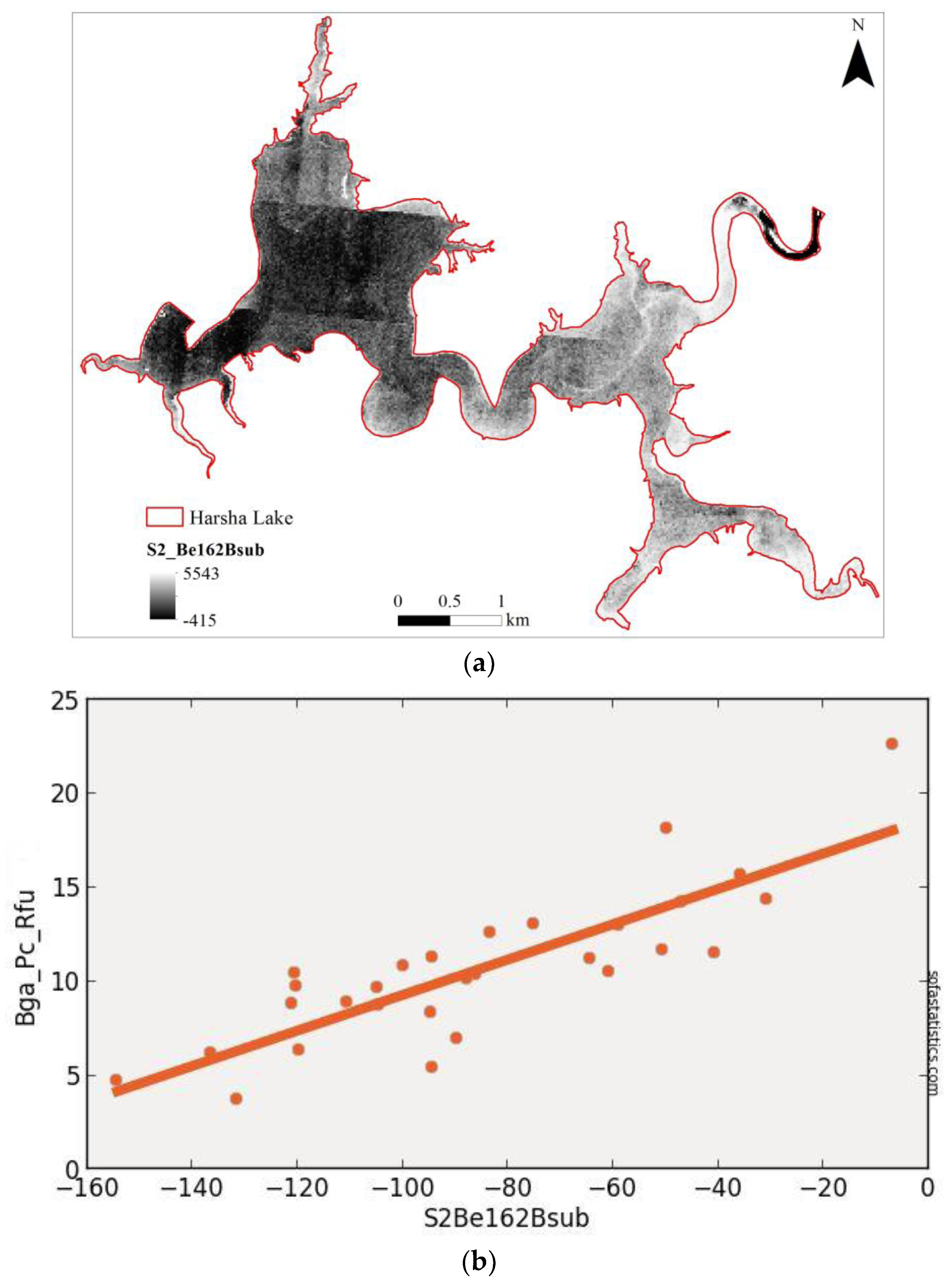
3.3. Sentinel-2 (Synthetic)
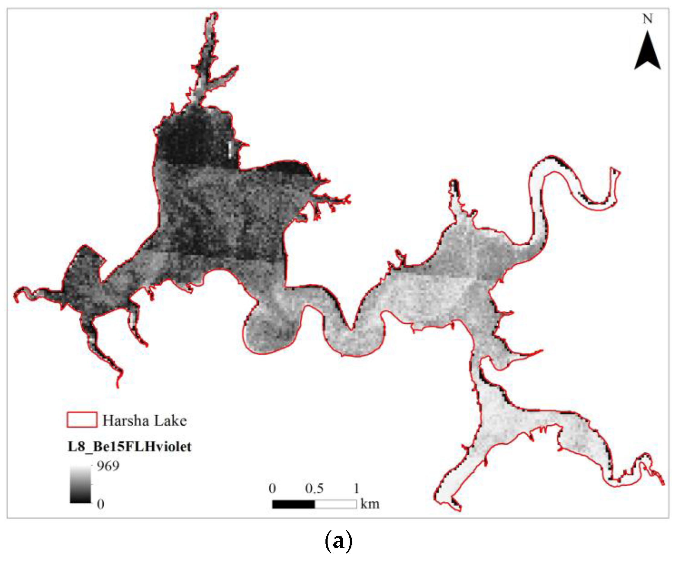
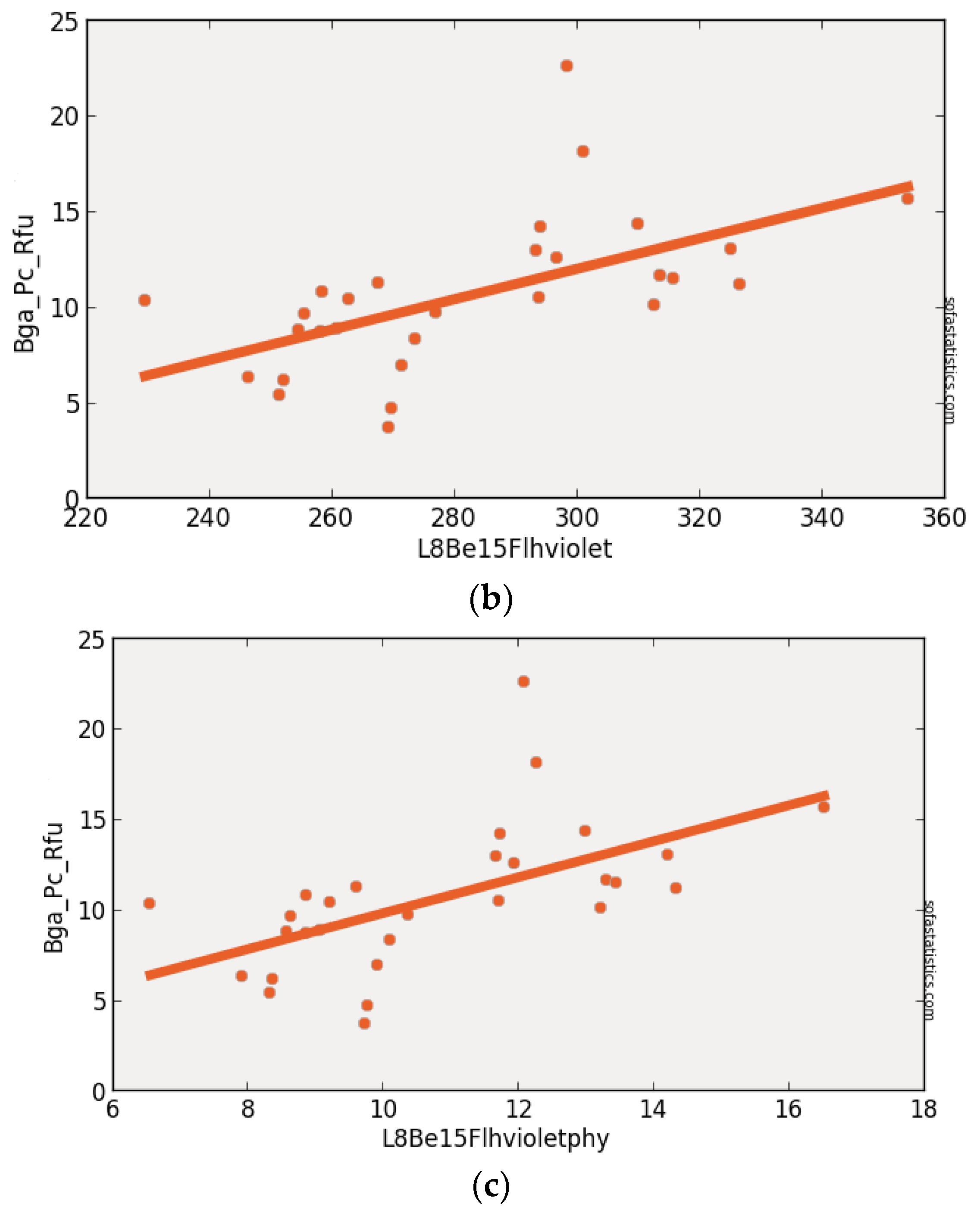
3.4. Landsat-8 (Synthetic)
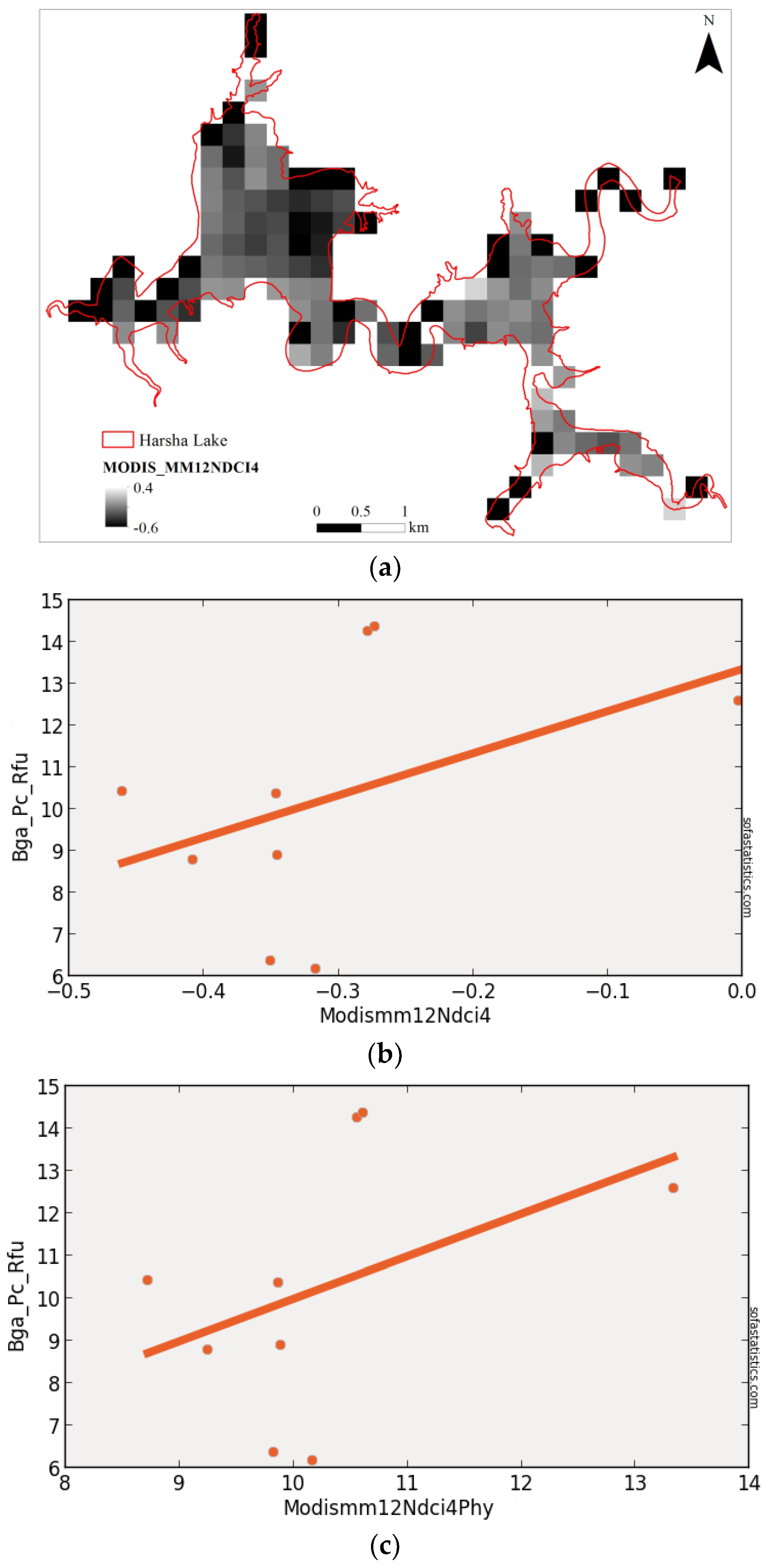
3.5. MODIS (Synthetic)
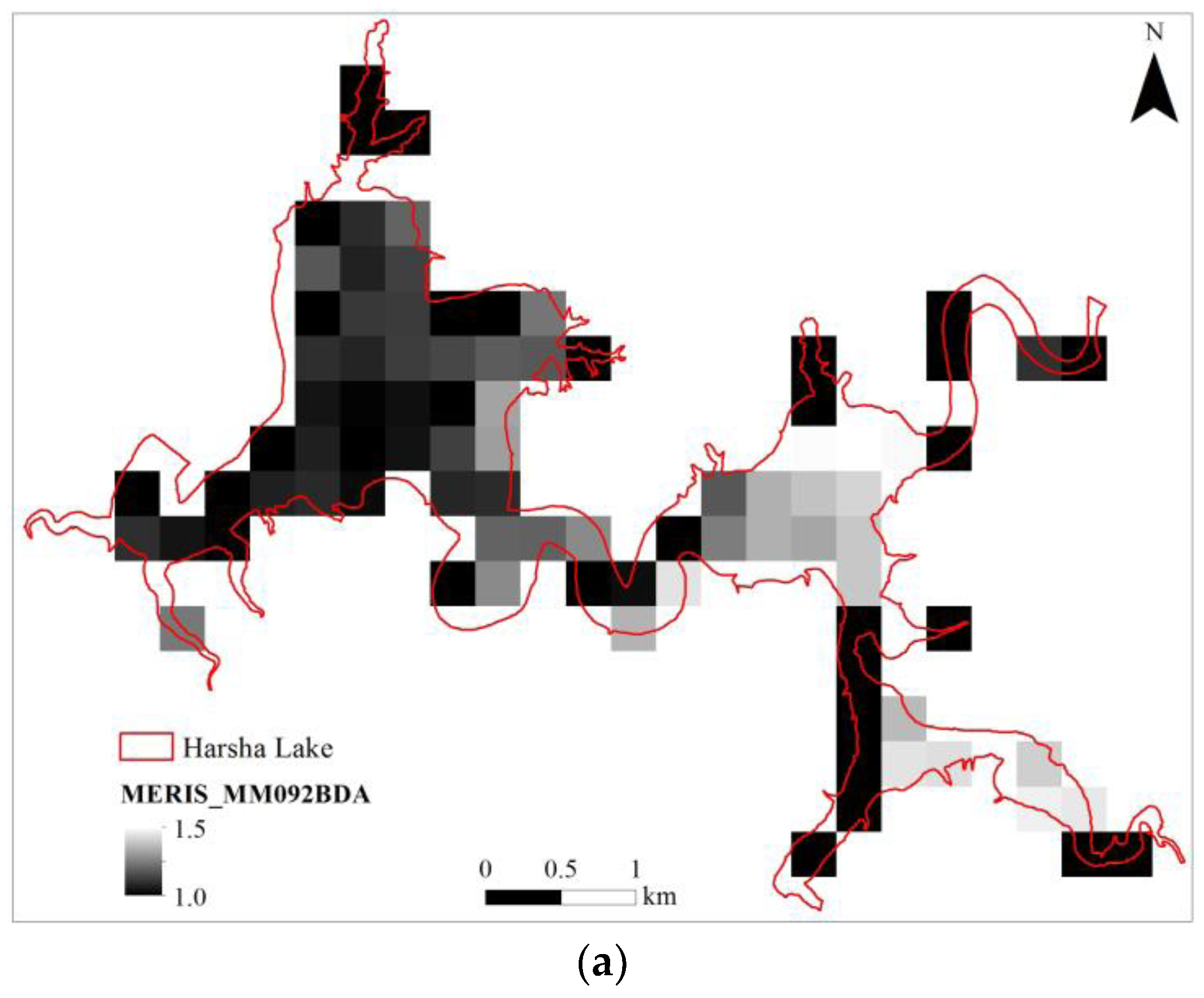
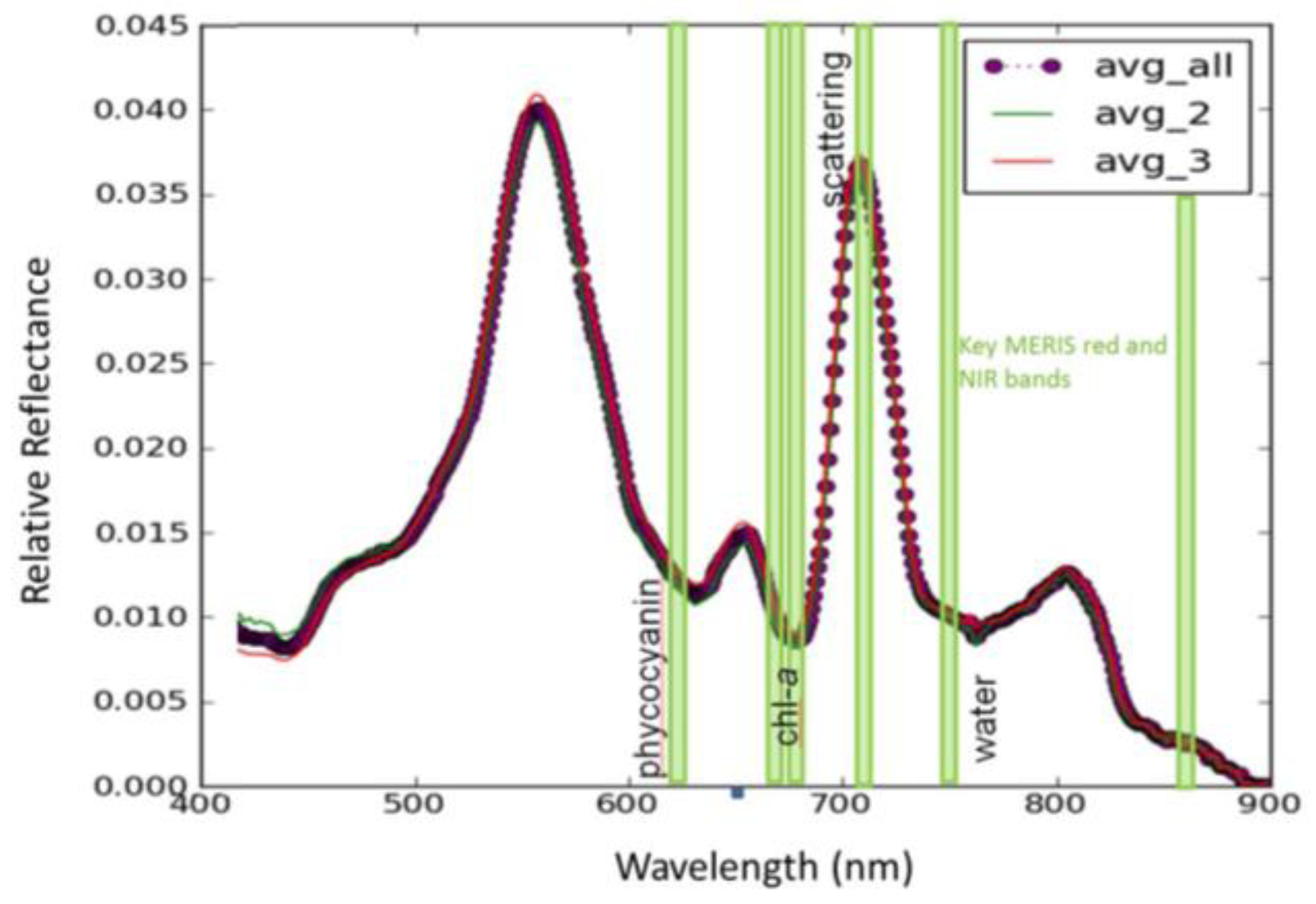
3.6. MERIS (Synthetic)
4. Discussion
5. Uncertainties, Errors and Accuracies
6. Conclusions
6.1. Best Performing Imager/Algorithm Combinations for BGA Estimation
6.2. Portability of Algorithms between Imagers
6.3. Implications for Operational BGA Monitoring with Existing and Near-Future Satellites
Supplementary Materials
Acknowledgments
Author Contributions
Conflicts of Interest
References
- Graham, J.L. Harmful Algal Blooms; USGS Fact Sheet, 2006-3147; USGS: Reston, VA, USA, 2006. [Google Scholar]
- Linkov, I.; Satterstrom, F.K.; Loney, D.; Steevans, J.A. The Impact of Harmful Algal Blooms on USACE Operations; ANSRP Technical Notes Collection; ERDC/TN ANSRP-09-1; U.S. Army Engineer Research and Development Center: Vicksburg, MS, USA, 2009. [Google Scholar]
- Matthews, M.W.; Bernard, S. Characterizing the absorption properties for remote sensing of three small optically-diverse South African reservoirs. Remote Sens. 2013, 5, 4370–4404. [Google Scholar] [CrossRef]
- Matthews, M.W.; Odermatt, D. Improved algorithm for routine monitoring of cyanobacteria and eutrophication in inland and near-coastal waters. Remote Sens. Environ. 2015, 156, 374–382. [Google Scholar] [CrossRef]
- Stumpf, R.P.; Wynne, T.T.; Baker, D.B.; Fahnenstiel, G.L. Interannual Variability of Cyanobacterial Blooms in Lake Erie. PLoS ONE 2012, 7, e42444. [Google Scholar] [CrossRef] [PubMed]
- Beck, R.A.; Zhan, S.; Liu, H.; Tong, S.; Yang, B.; Xu, M.; Ye, Z.; Huang, Y.; Wu, Q.; Wang, S.; et al. Comparison of satellite reflectance algorithms for estimating chlorophyll-a in a temperate reservoir using coincident hyperspectral aircraft imagery and dense coincident surface observations. Remote Sens. Environ. 2016, 178, 15–30. [Google Scholar] [CrossRef]
- Simis, S.G.H.; Peters, S.W.M.; Gons, H.J. Remote sensing of the cyanobacteria pigment phycocyanin in turbid inland water. Limnol. Oceanogr. 2005, 50, 237–245. [Google Scholar] [CrossRef]
- Simis, S.G.H.; Ruiz-Verdu, A.; Dominguez, J.A.; Pena-Martinez, R.; Peters, S.W.M.; Gons, H.J. Influence of phytoplankton pigment composition on remote sensing of cyanobacterial biomass. Remote Sens. Environ. 2007, 106, 414–427. [Google Scholar] [CrossRef]
- Randolph, K.; Wilson, J.; Tedesco, L.; Li, L.; Lani Pascual, D.; Soyeux, E. Hyperspectral remote sensing of cyanobacteria in turbid productive water using optically active pigments, chlorophyll a and phycocyanin. Remote Sens. Environ. 2008, 112, 4009–4019. [Google Scholar] [CrossRef]
- Ruiz-Verdu, A.; Simis, S.G.H.; de Hoyos, C.; Gons, H.J.; Pena-Martinez, R. An evaluation of algorithms for the remote sensing of cyanobacterial biomass. Remote Sens. Environ. 2008, 112, 3996–4008. [Google Scholar] [CrossRef]
- Mishra, S.; Mishra, D.R.; Schluchter, W.M. A novel algorithm for predicting PC concentrations in cyanobacteria: A proximal hyperspectral remote sensing approach. Remote Sens. 2009, 1, 758–775. [Google Scholar] [CrossRef]
- Klemas, V. Remote sensing of algal blooms: An overview with case studies. J. Coast. Res. 2012, 28, 34–43. [Google Scholar] [CrossRef]
- Mishra, S.; Mishra, D.R.; Lee, Z.P. Bio-optical inversion in highly turbid and cyanobacteria dominated waters. IEEE Trans. Geosci. Remote Sens. 2014, 52, 375–388. [Google Scholar] [CrossRef]
- Ogashawara, I.; Misra, D.R.; Mishra, S.; Curtarelli, M.P.; Stech, J.L. A performance review of reflectance based algorithms for predicting phycocyanin concentrations in inland waters. Remote Sens. 2013, 5, 4774–4798. [Google Scholar] [CrossRef]
- Lyu, H.; Wang, Q.; Wu, C.; Zhu, L.; Yin, B.; Li, Y.; Huang, J. Retrieval of phycocyanin concentration from remote-sensing reflectance using a semi-analytic model in eutrophic lakes. Ecol. Inform. 2013, 18, 178–187. [Google Scholar] [CrossRef]
- Mishra, S.; Mishra, D.R. A novel remote sensing algorithm to quantify phycocyanin in cyanobacterial algal blooms. Environ. Res. Lett. 2014, 9, 114003. [Google Scholar] [CrossRef]
- Kudela, R.M.; Palacios, S.L.; Austerberry, D.C.; Accorsi, E.K.; Guild, L.S.; Torres-Perez, J. Application of hyperspectral remote sensing to cyanobacterial blooms in inland waters. Remote Sens. Environ. 2015, 167, 196–205. [Google Scholar] [CrossRef]
- Lunetta, R.S.; Schaeffer, B.A.; Stumpf, R.P.; Keith, D.; Jacobs, S.A.; Murphy, M.S. Evaluation of cyanobacterial cell count detection derived from MERIS imagery across the eastern USA. Remote Sens. Environ. 2015, 157, 24–34. [Google Scholar] [CrossRef]
- Wynne, T.T.; Stumpf, R.P.; Tomlinson, M.C.; Warner, R.A.; Tester, P.A.; Dyble, J. Relating spectral shape to cyanobacterial blooms in the Laurentian Great Lakes. Int. J. Remote Sens. 2008, 29, 3665–3672. [Google Scholar] [CrossRef]
- Wynne, T.T.; Stumpf, R.P.; Tomlinson, M.C.; Dyble, J. Characterizing a cyanobacterial bloom in western Lake Erie using satellite imagery and meteorological data. Limnol. Oceanogr. 2012, 55, 2025–2036. [Google Scholar] [CrossRef]
- Wynne, T.T.; Stumpf, R.P. Spatial and Temporal Patterns in the Seasonal Distribution of Toxic Cyanobacteria in Western Lake Erie from 2002–2014. Toxins 2015, 7, 1649–1663. [Google Scholar] [CrossRef] [PubMed]
- Sun, D.; Hu, C.; Qiu, Z.; Shi, K. Estimating phycocyanin pigment concentration in productive inland waters using Landsat measurements: A case study in Lake Dianchi. Opt. Express 2015, 23, 3055–3074. [Google Scholar] [CrossRef] [PubMed]
- Wozniak, M.; Bradtke, K.M.; Darecki, M.; Krezel, A. Empirical Model for Phycocyanin Concentration Estimation as an Indicator of Cyanobacterial Bloom in the Optically Complex Coastal Waters of the Baltic Sea. Remote Sens. 2016, 8, 1–23. [Google Scholar] [CrossRef]
- Stumpf, R.P.; Davis, T.W.; Wynne, T.T.; Graham, J.L.; Loftin, K.A.; Johengen, T.H.; Gossiaux, D.; Palladino, D.; Burtner, A. Challenges for mapping cyanotoxin patterns from remote sensing of cyanobacteria. Harmful Algae 2016, 54, 160–173. [Google Scholar] [CrossRef] [PubMed]
- Morel, A.; Prieur, L. Analysis of variations in ocean color. Limnol. Oceanogr. 1977, 22, 709–722. [Google Scholar] [CrossRef]
- Dekker, A. Detection of the Optical Water Quality Parameters for Eutrophic Waters by High Resolution Remote Sensing. Ph.D. Thesis, Free University, Amsterdam, The Netherlands, 1993. [Google Scholar]
- Stumpf, R.P. Satellite Monitoring of Toxic Cyanobacteria for Public Health. Earthzine. 2014. Available online: http://earthzine.org/2014/03/26/satellite-monitoring-of-toxic-cyanobacteria-for-public-health/ (accessed on 7 April 2016).
- Augusto-Silva, P.B.; Ogashawara, I.; Barbosa, C.C.F.; de Carvalho, L.A.S.; Jorge, D.S.F.; Fornari, C.I.; Stech, J.L. Analysis of MERIS reflectance algorithms for estimating chlorophyll-a concentration in a Brazilian Reservoir. Remote Sens. 2014, 6, 11689–11707. [Google Scholar] [CrossRef]
- Hunter, P.D.; Tyler, A.N.; Willby, N.J.; Gilvear, D.J. The spatial dynamics of vertical migration by Microcystis aeruginosa in a eutrophic shallow lake: A case study using high spatial resolution time-series airborne remote sensing. Limnol. Oceanogr. 2008, 53, 2391–2406. [Google Scholar] [CrossRef]
- Wheeler, S.M.; Morrissey, L.A.; Levine, S.N.; Livingston, G.P.; Vincent, W.F. Mapping cyanobacterial blooms in Lake Champlain’s Missisquoi Bay using QuickBird and MERIS satellite data. J. Great Lakes Res. 2012, 38, 68–75. [Google Scholar] [CrossRef]
- Lee, Z.P.; Carder, K.L. Absorption spectrum of phytoplankton pigments derived from hyperspectral remote-sensing reflectance. Remote Sens. Environ. 2004, 89, 361–368. [Google Scholar] [CrossRef]
- Mishra, S.; Mishra, D.R. Normalized difference chlorophyll index: A novel model for remote estimation of chlorophyll-a concentration in turbid productive waters. Remote Sens. Environ. 2012, 117, 394–406. [Google Scholar] [CrossRef]
- Shen, L.; Xu, H.; Guo, X. Satellite remote sensing of harmful algal blooms (HABs) and a Potential Synthesized Framework. Sensors 2012, 12, 7778–7803. [Google Scholar] [CrossRef] [PubMed]
- Verbyla, D.L. Satellite Remote Sensing of Natural Resources; CRC Lewis: Boca Raton, FL, USA, 1995; p. 199. [Google Scholar]
- Gitelson, A.A.; Garbuzov, G.; Szilagyi, F.; Mittenzwey, K.H.; Karnieli, A.; Kaiser, A. Quantitative remote sensing methods for real-time monitoring of inland waters quality. Int. J. Remote Sens. 1993, 14, 1269–1295. [Google Scholar] [CrossRef]
- Fraser, R.N. Hyperspectral remote sensing of turbidity and chlorophyll a among Nebraska Sand Hills lakes. Int. J. Remote Sens. 1998, 19, 1579–1589. [Google Scholar] [CrossRef]
- Glasgow, H.B.; Burkholder, J.M.; Reed, R.E.; Lewitus, A.J.; Kleinman, J.E. Real-time remote monitoring of water quality: A review of current applications, and advancements in sensor technology, telemetry, and computing technologies. J. Exp. Mar. Biol. Ecol. 2004, 300, 409–448. [Google Scholar] [CrossRef]
- Binding, C.E.; Greenberg, T.A.; Bukata, R.P. The MERIS Maximum Chlorophyll Index; its merits and limitations for inland water algal bloom monitoring. J. Great Lakes Res. 2013, 39, 100–107. [Google Scholar] [CrossRef]
- Sawaya, K.E.; Olmanson, L.G.; Heinart, N.J.; Brezonik, P.L.; Bauer, M.E. Extending satellite remote sensing to local scales: Land and water resource monitoring using high-resolution imagery. Remote Sens. Environ. 2003, 88, 144–156. [Google Scholar] [CrossRef]
- Mayo, M.; Gitelson, A.A.; Yacobi, Y.Z.; Ben-Avraham, Z. Chlorophyll distribution in Lake Kinneret determined from Landsat Thematic Mapper data. Int. J. Remote Sens. 1995, 16, 175–182. [Google Scholar] [CrossRef]
- Alawadi, F. Detection of surface algal blooms using the newly developed algorithm surface algal bloom index (SABI). Proc. SPIE 2010, 7825. [Google Scholar] [CrossRef]
- Amin, R.; Zhou, J.; Gilerson, A.; Gross, B.; Moshary, F.; Ahmed, S. Novel optical techniques for detecting and classifying toxic dinoflagellate Karenia brevis blooms using satellite imagery. Opt. Express 2009, 17, 9126–9144. [Google Scholar] [CrossRef] [PubMed]
- Gitelson, A.A.; Gritz, U.; Merzlyak, M.N. Relationships between leaf chlorophyll content and spectral reflectance and algorithms for non-destructive chlorophyll assessment in higher plant leaves. J. Plant Phys. 2003, 160, 271–282. [Google Scholar] [CrossRef] [PubMed]
- Gower, J.; King, S.; Goncalves, P. Global monitoring of plankton blooms using MERIS MCI. Int. J. Remote Sens. 2008, 29, 6209–6216. [Google Scholar] [CrossRef]
- Kneubuhler, M.; Frank, T.; Kellenberger, T.W.; Pasche, N.; Schmid, M. Mapping chlorophyll-a in Lake Kivu with remote sensing methods. In Proceedings of the Envisat Symposium 2007, Montreux, Switzerland, 23–27 April 2007. [Google Scholar]
- Mishra, S. Remote Sensing of Harmful Algal Bloom. PhD Thesis, Mississippi State University, Starkville, MI, USA, 2012. [Google Scholar]
- Schalles, J.; Yacobi, Y. Remote detection and seasonal patterns of phycocyanin, carotenoid and chlorophyll-a pigments in eutrophic waters. Arch. Hydrobiol. Adv. Limnol. 2000, 55, 153–168. [Google Scholar]
- Peltzer, E.T. Model 1 and Model 2 Regressions. 2015. Available online: http://www.mbari.org/staff/etp3/regress.htm (accessed on 27 April 2015).
- Pinero, G.; Perelman, S.; Guerschman, J.P.; Paruleo, J.M. How to evaluate models: Observed vs. predicted or predicted vs. observed. Ecol. Model. 2008, 216, 316–322. [Google Scholar] [CrossRef]
- Lindsey, R.; Herring, D. Modis; 2001; pp. 1–23. Available online: https://modis.gsfc.nasa.gov/about/media/modis_brochure.pdf (accessed on 24 May 2017).
- Lee, Z.; Ahn, Y.-H.; Mobley, C.; Arnone, R. Removal of surface-reflected light for the measurement of remote-sensing reflectance from an above-surface platform. Opt. Express 2010, 18, 26313–26324. [Google Scholar] [CrossRef] [PubMed]
- Gao, B.; Montes, M.J.; Davis, C.O.; Goetz, A.H. Atmospheric correction algorithms for hyperspectral remote sensing data of land and ocean. Remote Sens. Environ. 2009, 113, S17–S24. [Google Scholar] [CrossRef]
- Reif, M. Remote Sensing for Inland Water Quality Monitoring: A U.S. Army Corps of Engineers Perspective; Engineer Research and Development Center/Environmental Laboratory Technical Report (ERDC/EL TR)-11-13; Engineer Research and Development Center/Environmental Laboratory: Vicksburg, MS, USA, 2011. [Google Scholar]


| Imager | Original Range (nm) | Center (nm) | FWHM (nm) | Synthetic Range (nm) | Synthetic Center (nm) | FWHM (nm) |
|---|---|---|---|---|---|---|
| WorldView-2/3 | Resampled to 1.8 m | |||||
| b1 | 400–450 | 425 | 50 | 403–454 | 428.5 | 51 |
| b2 | 450–510 | 480 | 60 | 454–505 | 479.5 | 51 |
| b3 | 510–580 | 545 | 70 | 523–573 | 548 | 50 |
| b4 | 585–625 | 605 | 40 | 582–633 | 607.5 | 51 |
| b5 | 630–690 | 660 | 60 | 634–684 | 659 | 50 |
| b6 | 705–745 | 725 | 40 | 710–749 | 729.5 | 39 |
| b7 | 770–895 | 832.5 | 125 | 790–889 | 839.5 | 99 |
| b8 | 860–1040 | 950 | 180 | 889–1043 | 966 | 154 |
| Sentinel-2 | Resampled to 20 m | |||||
| b1 | 433–453 | |||||
| b2 | 458–523 | 490.5 | 65 | 457–515 | 486 | 58 |
| b3 | 543–578 | 560.5 | 35 | 543–572 | 557.5 | 29 |
| b4 | 650–680 | 665 | 30 | 643–686 | 664.5 | 43 |
| b5 | 698–713 | 705.5 | 15 | 700–714 | 707 | 14 |
| b6 | 733–748 | 740.5 | 15 | 728–743 | 735.5 | 15 |
| b7 | 773–793 | 783 | 20 | 771–800 | 785.5 | 29 |
| b8 | 785–900 | 842.5 | 115 | 785–900 | 842.5 | 115 |
| b8b | 855–875 | 865 | 20 | 856–871 | 863.5 | 15 |
| b9 | 935–955 | 945 | 20 | 935–955 | 945 | 20 |
| Landsat-8 | Resampled to 30 m | |||||
| b1 | 430–450 | 440 | 20 | 429–443 | 436 | 14 |
| b2 | 450–510 | 480 | 60 | 457–500 | 478.5 | 43 |
| b3 | 530–590 | 560 | 60 | 529–586 | 557.5 | 57 |
| b4 | 640–670 | 655 | 30 | 643–672 | 657.5 | 29 |
| b5 | 850–880 | 865 | 30 | 856–885 | 870.5 | 29 |
| MODIS | Resampled to 250 m | |||||
| b1 | 620–670 | 645 | 50 | 615–672 | 643.5 | 57 |
| b2 | 841–876 | 858.5 | 35 | 842–871 | 856.5 | 29 |
| S3/MERIS/OLCI | Resampled to 300 m | |||||
| b1 | 402–412 | 407 | 10 | 400–414 | 407 | 14 |
| b2 | 438–448 | 443 | 10 | 429–457 | 443 | 28 |
| b3 | 485–495 | 490 | 10 | 486–500 | 493 | 14 |
| b4 | 505–515 | 510 | 10 | 500–515 | 507.5 | 15 |
| b5 | 555–565 | 560 | 10 | 558–572 | 565 | 14 |
| b6 | 615–625 | 620 | 10 | 615–629 | 622 | 14 |
| b7 | 660–670 | 665 | 10 | 657–672 | 664.5 | 15 |
| b8 | 678–685 | 681.5 | 7 | 672–686 | 679 | 14 |
| b9 | 704–714 | 709 | 10 | 700–714 | 707 | 14 |
| b10 | 750–757 | 753.5 | 7 | 743–757 | 750 | 14 |
| b11 | 757–762 | 759.5 | 5 | 750–764 | 757 | 14 |
| b12 | 772–787 | 779.5 | 15 | 757–800 | 778.5 | 43 |
| b13 | 855–875 | 865 | 20 | 842–885 | 863.5 | 43 |
| b14 | 880–890 | 885 | 10 | 871–899 | 885 | 28 |
| b15 | 895–905 | 900 | 10 | 885–913 | 899 | 28 |
| Algorithm | Reference | ENVI Band Math with Original Specified Wavelengths |
|---|---|---|
| (Numerical Value = Wavelength in nm) | ||
| Al10SABI | Alawadi et al. (2010) [41] | (float(857) − float(644))/(float(458) + float(529)) |
| Am092Bsub | Amin et al. (2009) [42] | (float(678)) − (float(667)) |
| Am09KBBI | Amin et al. (2009) [42] | (float(686) − float(658))/(float(686) + float(658)) |
| Be162Bdiv | This paper | (float(681))/(float(665)) |
| Be162Bsub * | This paper | (float(700)) − (float(622)) |
| Be16FLHblue | Beck et al. (2016) [6] | (float(529)) − [float(644) + (float(458) − float(644))] |
| Be16FLHPhy * | This paper | (float(620)) − [float(709) + (float(560) − float(709))] |
| Be16FLHviolet | Beck et al. (2016) [6] | (float(529)) − [float(644) + (float(5) − float(644))] |
| Be16NDPhyI * | This paper | (float(700) − float(622))/(float(700) + float(622)) |
| DE933BDA | Dekker (1993) [26] | ((float(600)) − (float(648))) − (float(625)) |
| Gi033BDA | Gitelson et al. (2003) [43] | ((1/float(672)) − (1/float(715))) × (float(757)) |
| Go04MCI | Gower et al. (2004) [44] | (((float(709)) − (float(681)) − ((float(753)) − (float(681))))) |
| HU103BDA * | Hunter et al. (2008) [29] | ((1/float(615)) − (1/float(600))) − (float(725)) |
| Kn07KIVU | Kneubuhler et al. (2007) [45] | (float(458) − float(644))/(float(529)) |
| Ku15PhyCI | Kudela et al. (2015) [17] | −1 × (((float(681)) − (float(665)) − ((float(709)) − (float(665))))) |
| MI092BDA | Mishra et al. (2009) [11] | (float(700))/(float(600)) |
| MM092BDA | Mishra et al. (2009) [11] | (float(724))/(float(600)) |
| MM12NDCI | Mishra and Mishra (2012) [32] | (float(700) − float(665))/(float(700) + float(665)) |
| MM143BDAopt * | Mishra and Mishra (2014) [16] | ((1/float(629)) − (1/float(659))) × (float(724)) |
| MM143BDAver3merisver * | Mishra and Mishra (2014) [16] | ((1/float(620)) − (1/float(665))) × (float(778)) |
| SI052BDA * | Simis et al. (2005) [7] | (float(709))/(float(620)) |
| SM122BDA | S. Mishra (2012) [46] | (float(709))/(float(600)) |
| SY002BDA * | Schalles and Yacobi (2000) [47] | (float(650))/(float(625)) |
| Stu16Phy | Stumpf et al. (2016) [24] | (float(665) − float(620)) + ((float(620) − float(681)) × 0.74) |
| Stu16PhyFLH * | Stumpf et al. (2016) [24] | (float(665)) − (float(681) + (float(620) − float(681))) |
| Wy08CI | Wynne et al. (2008) [19] | −1 × (((float(686)) − (float(672)) − ((float(715)) − (float(672))))) |
| Zh10FLH | Zhao et al. (2010) [48] | (float(686)) − [float(715) + (float(672) − float(715))] |
| Algorithms By Satellite/Sensor | R-Squared | Adj. R-Sqr. | Std. Err. Reg. | Std. Dev. | n | Residual Mean Square | p | Conf. Level |
|---|---|---|---|---|---|---|---|---|
| S | ||||||||
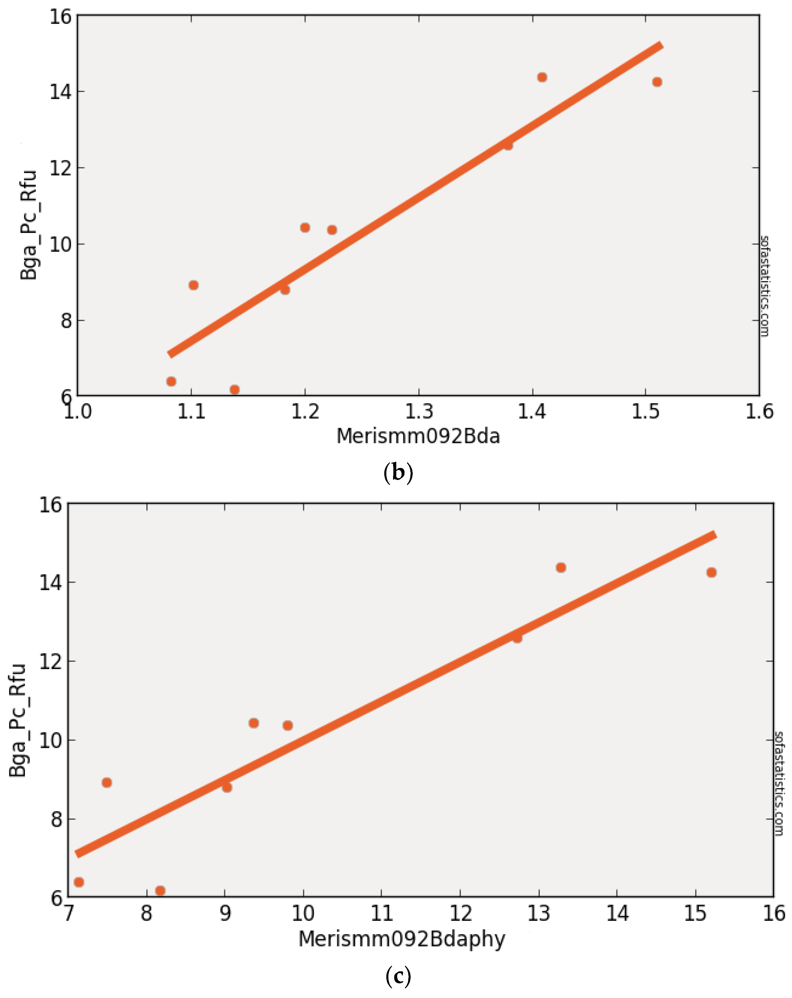
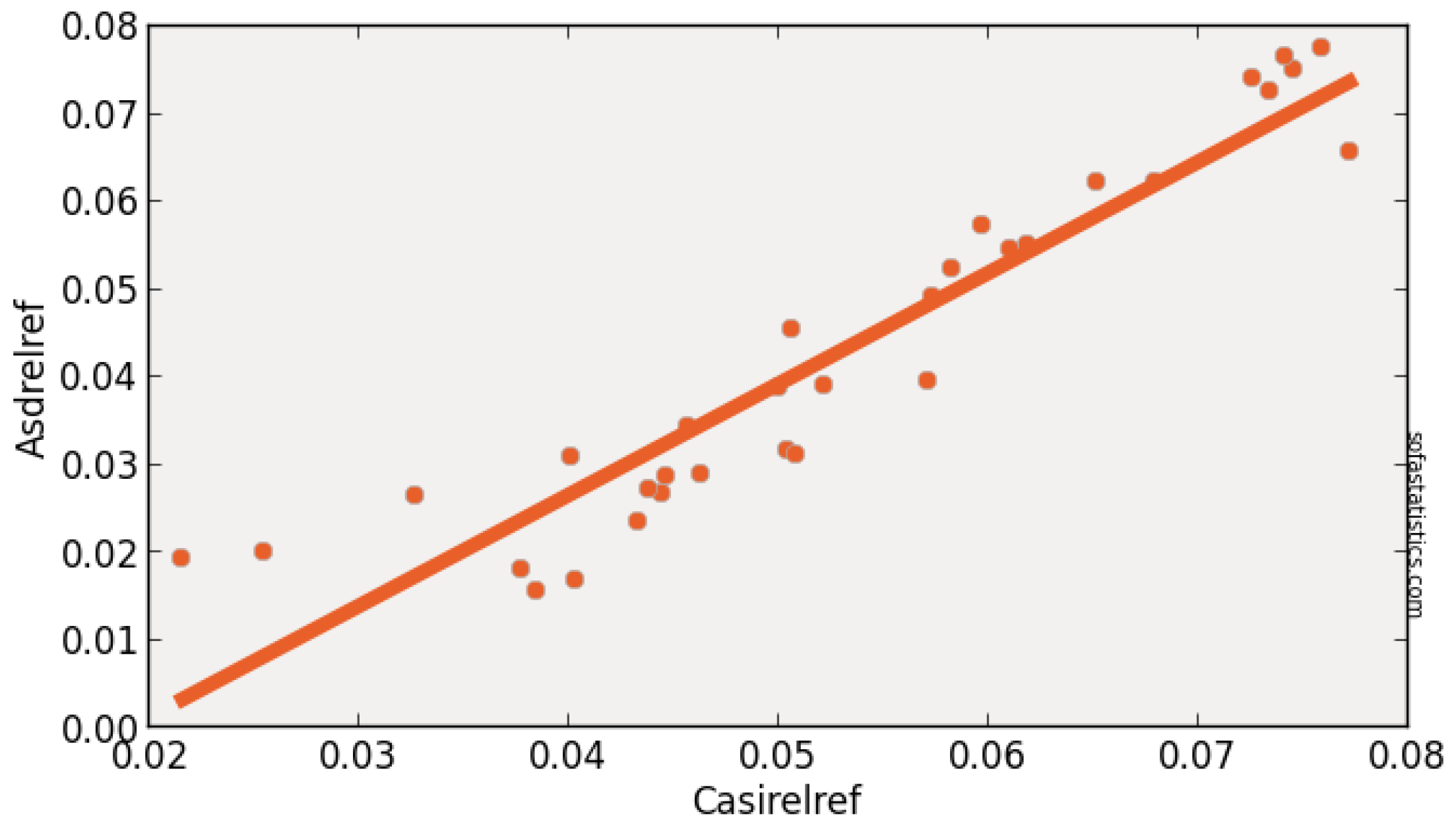
| CASIBe152BsubPhy715sub615 | 0.763 | 0.754 | 1.974 | 3.978 | 29 | 3.896 | <0.001 | 95.0% |
| (float(715)) − (float(615)) | ||||||||
| WV2Be162Bsub | 0.790 | 0.782 | 1.871 | 4.007 | 29 | 3.500 | <0.001 | 95.0% |
| (float(730)) − (float(608)) | ||||||||
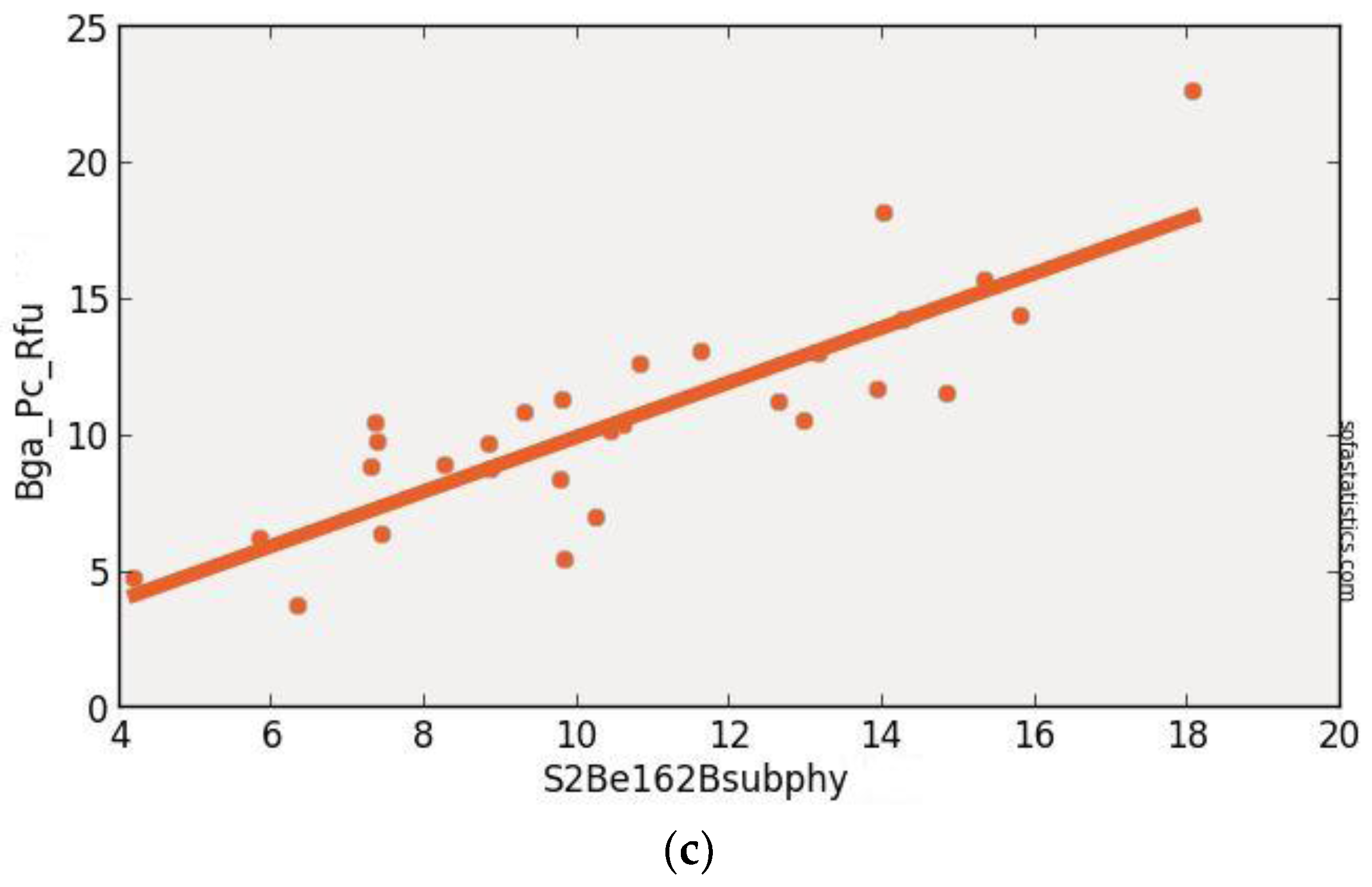
| S2Be162Bsub | 0.704 | 0.693 | 2.219 | 4.007 | 29 | 4.924 | <0.001 | 95.0% |
| (float(736)) − (float(665)) | ||||||||
| L8Be15Flhviolet | 0.339 | 0.314 | 3.318 | 4.007 | 29 | 11.011 | <0.001 | 95.0% |
| (float(530)) − [float(640) + (float(430) − float(640))] | ||||||||
| MODISMM12NDCI4 | 0.183 | 0.066 | 2.938 | 3.040 | 9 | 8.632 | 0.251 | 95.0% |
| (float(857) − float(644))/(float(857) + float(644)) | ||||||||
| MERISMM092BDA | 0.863 | 0.843 | 1.203 | 3.040 | 9 | 1.448 | <0.001 | 95.0% |
| (float(707))/(float(679)) |
| Algorithms By Satellite/Sensor | Spatial | n | Geometric | Geometric | Geometric | Geometric | Standard | Standard |
|---|---|---|---|---|---|---|---|---|
| (Band Math in nm) | Res. (m) | Mean | Mean | Mean | Mean | Deviation of | Deviation of | |
| Slope | Intercept | Correlation | Correlation | Slope | Y-intercept | |||
| Coefficient | Coefficient | |||||||
| Squared | ||||||||
| CASIBe152BsubPhy715sub615 | 1 | 29 | 1.141 | −1.500 | 0.881 | 0.777 | 0.107 | 1.199 |
| (float(715)) − (float(615)) | ||||||||
| WV2Be162Bsub | 1.8 | 29 | 1.128 | −1.376 | 0.889 | 0.790 | 0.102 | 1.150 |
| (float(730)) − (float(608)) | ||||||||
| S2Be162Bsub | 20 | 29 | 1.194 | −2.087 | 0.839 | 0.704 | 0.130 | 1.456 |
| (float(736)) − (float(665)) | ||||||||
| L8Be15Flhviolet | 30 | 29 | 1.708 | −7.773 | 0.582 | 0.339 | 0.301 | 3.317 |
| (float(530)) − [float(640) + (float(430) − float(640))] | ||||||||
| MODISMM12NDCI412 | 250 | 9 | 2.339 | −13.716 | 0.428 | 0.183 | 0.946 | 9.760 |
| (float(857) − float(644))/(float(857) + float(644)) | ||||||||
| MERISMM092BDA | 300 | 9 | 1.077 | −0.783 | 0.929 | 0.863 | 0.153 | 1.624 |
| (float(707))/(float(679)) |
| Constituent (unit) | Description |
|---|---|
| Alkalinity mg as CaCO3 | as is |
| BGA-PC-Cells/mL | BlueGreen Algae (Cyanobacteria) probe response as cell density |
| BGA-PC-RFU | BlueGreen Algae (Cyanobacteria) probe response as relative fluorescence unit |
| Chl-µg/L | Chlorophyll probe response as concentration |
| Chl-RFU | Chlorophyll probe response as relative fluorescence unit |
| Depth-m | as is |
| DNH4 (ugN/L) | Dissolved Ammonium |
| DNO2-3 (ugN/L) | Dissolved Nitrite-Nitrate |
| DOC (mg/L) | Dissolved organic Carbon |
| DRP (ugP/L) | Dissolved Reactive Phosphorous (or filtered Ortho-P) |
| hardness mg as CaCO3 | as is |
| HCO3- (est) (ppm) | Bicarbonate ion |
| MC-LR CV | Coefficient of variation of environmental sample run in triplicate |
| MC-LR Stdev (3reps) | Standard deviation of environmental sample run in triplicate |
| Microcystin-LR equivalent | Microcystin LR equivalents measured by ELISA as concentration (PPB) |
| ODO-mg/L | Optical Dissolved Oxygen probe measurement as concentration |
| ODO Sat % | Optical Dissolved Oxygen probe measurement as percent saturation |
| OM percent (% OM) | % organic matter of suspended solids |
| pH | as is |
| pH (@Alkalinity measurement) | as is |
| PN (ugN/L) | Particulate Nitrogen |
| POC (mg/L) | Particulate Organic Carbon |
| PP (ugP/L) | Particulate Phosphorous |
| PRP (ugP/L) | Particulate Reactive Phosphorous |
| RCe,a (ug/L) | Phaephyton Corrected Chlorophyll A measured as absorbance on filtered and extracted samples |
| RCHLa (ug/L) | Uncorrected Chlorophyll A measured as absorbance on filtered and extracted samples |
| RCHLb (ug/L) | Uncorrected Chlorophyll B measured as absorbance on filtered and extracted samples |
| RCHLc (ug/L) | Uncorrected Chlorophyll C measured as absorbance on filtered and extracted samples |
| RPe,a (ug/L) | Phaephyton measured as absorbance on filtered and extracted samples |
| Sonde Number | as is |
| SpCond-uS/cm | Specific Conductance in microsemens per cm |
| TDN (ugNL) | Total Dissolved Nitrogen |
| TDP (ugP/L) | Total Dissolved Phosphorous |
| Temp-°C | as is |
| Time | as is |
| TN (ugN/L) | Total Nitrogen |
| TNH4 (ugN/L) | Total Ammonium |
| TOC (mg/L) | Total Organic Carbon |
| TP (ugP/L) | Total Phosphorous |
| TRP (ugP/L) | Total Reactive Phosphorous (or Unfiltered Ortho-P) |
| TSS (mg/L) | Total Suspended Solids |
| Turbidity-NTU | as is |
| VSS (mg/L) | Volatile Suspended Solids |
| Constituent (Unit) | No. of Water | Pearson’s r | Pearson’s r2 | p Value | Slope | Intercept |
|---|---|---|---|---|---|---|
| Truth Sites | vs. BGA_RFU | vs. BGA_RFU | vs. BGA_RFU | vs. BGA_RFU | vs. BGA_RFU | |
| Alkalinity mg as CaCO3 | 44 | 0.736 | 0.542 | <0.001 | 0.401 | −22.727 |
| BGA-PC-Cells/mL | 44 | 1.000 | 1.000 | <0.001 | 0.000 | −0.245 |
| Chl-µg/L | 44 | 0.807 | 0.651 | <0.001 | 0.666 | 3.889 |
| Chl-RFU | 44 | 0.800 | 0.640 | <0.001 | 3.500 | 2.555 |
| DNO2-3 (ugN/L) | 44 | −0.097 | 0.009 | 0.530 | −0.058 | 10.833 |
| DOC (mg/L) | 44 | 0.361 | 0.130 | 0.016 | 7.673 | −41.867 |
| DRP (ugP/L) | 44 | 0.813 | 0.661 | <0.001 | 0.541 | 4.247 |
| hardness mg as CaCO3 | 44 | 0.540 | 0.292 | <0.001 | 0.264 | −17.696 |
| HCO3- (est) (ppm) | 44 | 0.742 | 0.551 | <0.001 | 0.593 | −31.110 |
| Microcystin-LR equivalent | 44 | 0.279 | 0.078 | 0.066 | 1.178 | 4.917 |
| Microcystin-LR equivalent 2–6.5 ppm | 44 | 0.665 | 0.442 | <0.001 | 6.105 | −17.233 |
| ODO-mg/L | 44 | 0.357 | 0.127 | 0.019 | 0.628 | −0.121 |
| ODO Sat % | 44 | 0.309 | 0.095 | 0.044 | 0.041 | 1.571 |
| OM percent (% OM) | 44 | −0.522 | 0.272 | <0.001 | −0.361 | 41.143 |
| pH | 44 | 0.475 | 0.226 | 0.001 | 8.531 | −74.903 |
| pH (@Alkalinity measurement) | 44 | 0.180 | 0.032 | 0.249 | 7.193 | −58.769 |
| PN (ugN/L) | 44 | 0.769 | 0.591 | <0.001 | 0.021 | −1.928 |
| POC (mg/L) | 44 | −0.053 | 0.003 | 0.734 | −1.503 | 11.308 |
| PP (ugP/L) | 44 | 0.835 | 0.697 | <0.001 | 0.200 | −3.672 |
| PRP (ugP/L) | 44 | 0.163 | 0.027 | 0.296 | 0.101 | 9.154 |
| RCe,a (ug/L) | 44 | 0.323 | 0.104 | 0.035 | 0.143 | 5.158 |
| RPe,a (ug/L) | 44 | 0.671 | 0.450 | <0.001 | 0.214 | 7.615 |
| SpCond-uS/cm | 44 | 0.505 | 0.255 | <0.001 | 0.225 | −47.140 |
| TDN (ugNL) | 44 | 0.156 | 0.024 | 0.317 | 0.017 | 0.626 |
| TDP (ugP/L) | 44 | 0.781 | 0.610 | <0.001 | 0.288 | 5.984 |
| Temp-°C | 44 | −0.497 | 0.247 | <0.001 | −3.136 | 101.334 |
| TN (ugN/L) | 44 | 0.810 | 0.656 | <0.001 | 0.022 | −15.515 |
| TNH4 (ugN/L) | 44 | −0.093 | 0.009 | 0.554 | −0.030 | 11.033 |
| TOC (mg/L) | 44 | 0.428 | 0.183 | 0.004 | 12.258 | −79.471 |
| TP (ugP/L) | 44 | 0.851 | 0.724 | <0.001 | 0.129 | −0.672 |
| TRP (ugP/L) | 44 | 0.667 | 0.445 | <0.001 | 0.301 | 2.952 |
| TSS (mg/L) | 44 | 0.888 | 0.789 | <0.001 | 1.545 | −5.619 |
| Turbidity-NTU | 44 | 0.923 | 0.852 | <0.001 | 1.319 | −8.609 |
| VSS (mg/L) | 44 | 0.816 | 0.666 | <0.001 | 2.025 | −7.280 |
© 2017 by the authors. Licensee MDPI, Basel, Switzerland. This article is an open access article distributed under the terms and conditions of the Creative Commons Attribution (CC BY) license (http://creativecommons.org/licenses/by/4.0/).
Share and Cite
Beck, R.; Xu, M.; Zhan, S.; Liu, H.; Johansen, R.A.; Tong, S.; Yang, B.; Shu, S.; Wu, Q.; Wang, S.; et al. Comparison of Satellite Reflectance Algorithms for Estimating Phycocyanin Values and Cyanobacterial Total Biovolume in a Temperate Reservoir Using Coincident Hyperspectral Aircraft Imagery and Dense Coincident Surface Observations. Remote Sens. 2017, 9, 538. https://doi.org/10.3390/rs9060538
Beck R, Xu M, Zhan S, Liu H, Johansen RA, Tong S, Yang B, Shu S, Wu Q, Wang S, et al. Comparison of Satellite Reflectance Algorithms for Estimating Phycocyanin Values and Cyanobacterial Total Biovolume in a Temperate Reservoir Using Coincident Hyperspectral Aircraft Imagery and Dense Coincident Surface Observations. Remote Sensing. 2017; 9(6):538. https://doi.org/10.3390/rs9060538
Chicago/Turabian StyleBeck, Richard, Min Xu, Shengan Zhan, Hongxing Liu, Richard A. Johansen, Susanna Tong, Bo Yang, Song Shu, Qiusheng Wu, Shujie Wang, and et al. 2017. "Comparison of Satellite Reflectance Algorithms for Estimating Phycocyanin Values and Cyanobacterial Total Biovolume in a Temperate Reservoir Using Coincident Hyperspectral Aircraft Imagery and Dense Coincident Surface Observations" Remote Sensing 9, no. 6: 538. https://doi.org/10.3390/rs9060538
APA StyleBeck, R., Xu, M., Zhan, S., Liu, H., Johansen, R. A., Tong, S., Yang, B., Shu, S., Wu, Q., Wang, S., Berling, K., Murray, A., Emery, E., Reif, M., Harwood, J., Young, J., Martin, M., Stillings, G., Stumpf, R., ... Huang, Y. (2017). Comparison of Satellite Reflectance Algorithms for Estimating Phycocyanin Values and Cyanobacterial Total Biovolume in a Temperate Reservoir Using Coincident Hyperspectral Aircraft Imagery and Dense Coincident Surface Observations. Remote Sensing, 9(6), 538. https://doi.org/10.3390/rs9060538