Abstract
We analyzed 27 established and new simple and therefore perhaps portable satellite phycocyanin pigment reflectance algorithms for estimating cyanobacterial values in a temperate 8.9 km2 reservoir in southwest Ohio using coincident hyperspectral aircraft imagery and dense coincident water surface observations collected from 44 sites within 1 h of image acquisition. The algorithms were adapted to real Compact Airborne Spectrographic Imager (CASI), synthetic WorldView-2, Sentinel-2, Landsat-8, MODIS and Sentinel-3/MERIS/OLCI imagery resulting in 184 variants and corresponding image products. Image products were compared to the cyanobacterial coincident surface observation measurements to identify groups of promising algorithms for operational algal bloom monitoring. Several of the algorithms were found useful for estimating phycocyanin values with each sensor type except MODIS in this small lake. In situ phycocyanin measurements correlated strongly (r2 = 0.757) with cyanobacterial sum of total biovolume (CSTB) allowing us to estimate both phycocyanin values and CSTB for all of the satellites considered except MODIS in this situation.
1. Introduction
1.1. Background
Algal blooms, including some toxic or “harmful” algal blooms (HABs), are increasing and affecting inland rivers, lakes and reservoirs, many of which are used as a source of drinking water [1,2]. HABs are often associated with prokaryotic cyanobacteria (i.e., blue-green algae (BGA)) [1]. These HABs have made the development of satellite reflectance algorithms for the estimation of the chlorophyll-a (Chl-a) and phycocyanin (PC) pigments associated with cyanobacterial biomass a high research priority for monitoring and warning efforts [3,4,5,6]. Chlorophyll-a is less specific to cyanobacterial blooms than phycocyanin because it occurs in both prokaryotic and eukaryotic phytoplankton, although Chl-a is more easily sensed by a variety of current and near-future satellite imaging systems because most current electro-optical satellite imaging systems are also designed to sense Chl-a in land plants [5].
Phycocyanin is a spectrally active accessory pigment specific to cyanobacteria that is commonly used as a proxy for cyanobacterial (BGA) biomass [4,7,8,9,10,11,12,13,14,15,16,17,18,19,20,21,22,23]. Phycocyanin pigment is therefore a key indicator of water quality [11,16]. Phycocyanin is more specific to cyanobacteria but is more difficult to sense because its spectral features are subtler and overlap with Chlorophyll-a, b and c as well as other pigments and water quality parameters [24]. Satellite reflectance algorithms for estimating BGA values with algorithms focused on phycocyanin reflectance signatures in temperate inland water bodies have been reviewed and evaluated by many researchers [10,11,14,16,22]. The large amount of previous BGA algorithm research has resulted in numerous algorithm options for algal bloom monitoring.
1.2. Rationale
The goal of this research is to find relatively simple, semi-analytical (spectral signature-based) phycocyanin and chlorophyll-a reflectance algorithms that are adaptable to a variety of satellite imagers (i.e., portable). A main objective is to maximize the utility of multiple current and near-future satellite imaging systems to counter the frequent cloud cover occurring over many small inland water bodies to estimate BGA/PC values. We conducted a case study using Harsha Lake, a 2000-acre (8.9 km2) drinking water reservoir in southwestern Ohio experiencing HABs. We began this research with a comparison of real aircraft and simulated satellite data imager/algorithm combinations against chlorophyll-a (Chl-a) coincident water surface observations [6]. We focus on BGA/PC estimation in this paper.
1.3. Study Area
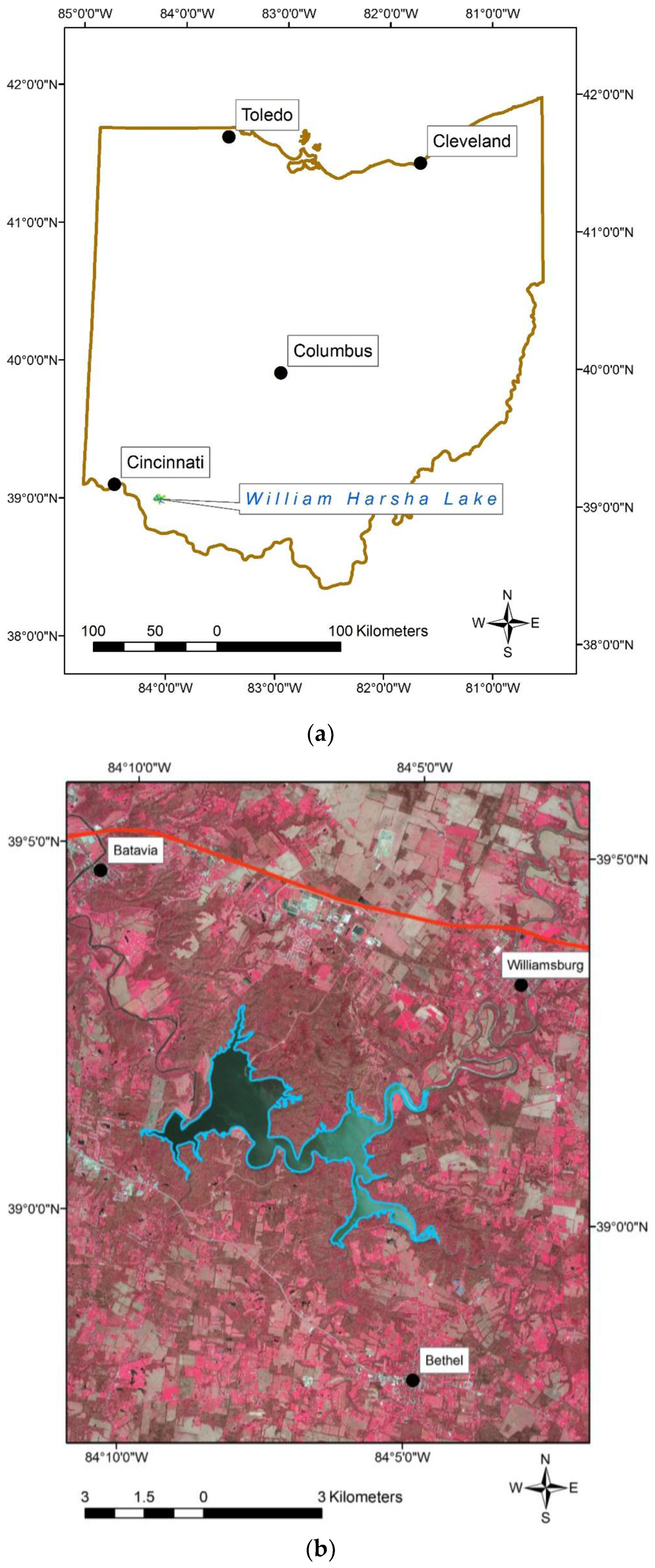
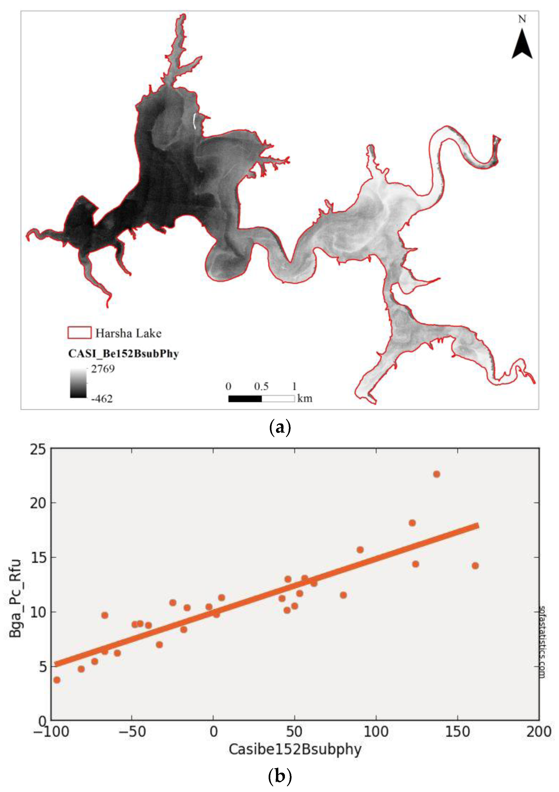
For the sake of brevity, most of the details of our approach, study area (Figure 1), aircraft campaign, pre-processing, synthetic satellite data construction, image analysis, statistical regression techniques, combined error budgets, and coincident surface observations (Figure 2) are available in our companion Chl-a study [6].
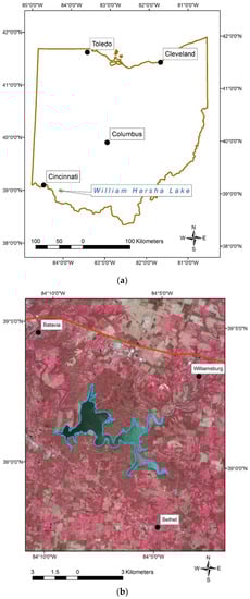
Figure 1.
Location maps of Harsha (East Fork) Lake near Cincinnati, Ohio: location in Ohio (a); and in detail (b).
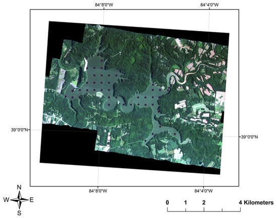
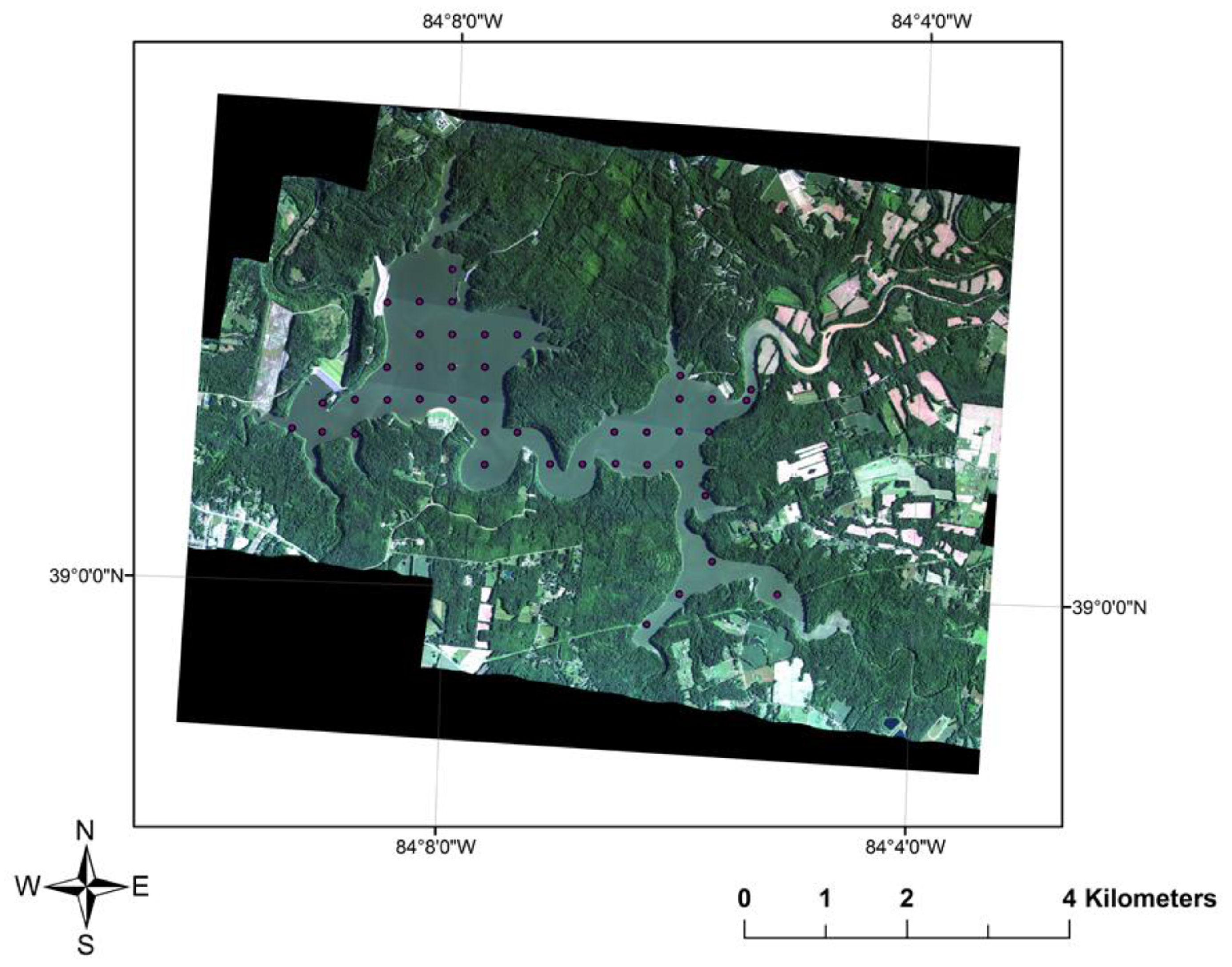
Figure 2.
Image of Harsha (East Fork) Lake acquired with a CASI-1500 imager on 27 June 2014 with 44 coincident surface observation locations used in this study.
1.4. Approach
Phycocyanin is a light blue organic compound more specific to cyanobacterial (BGA/PC) values than chlorophyll-a [16]. The phycocyanin reflectance signature when compared to that of Chl-a is both weaker [24] and more difficult to sense directly with most imagers due to the interfering reflectance of chlorophyll-a and other spectrally active substances in water with abundant phytoplankton and/or sediment [7,8] (Figure 3). This interference makes the width and spacing of spectral bands for each imager important with regard to avoiding other spectral components [7,8,10,11,13,14,16,24,25,26].

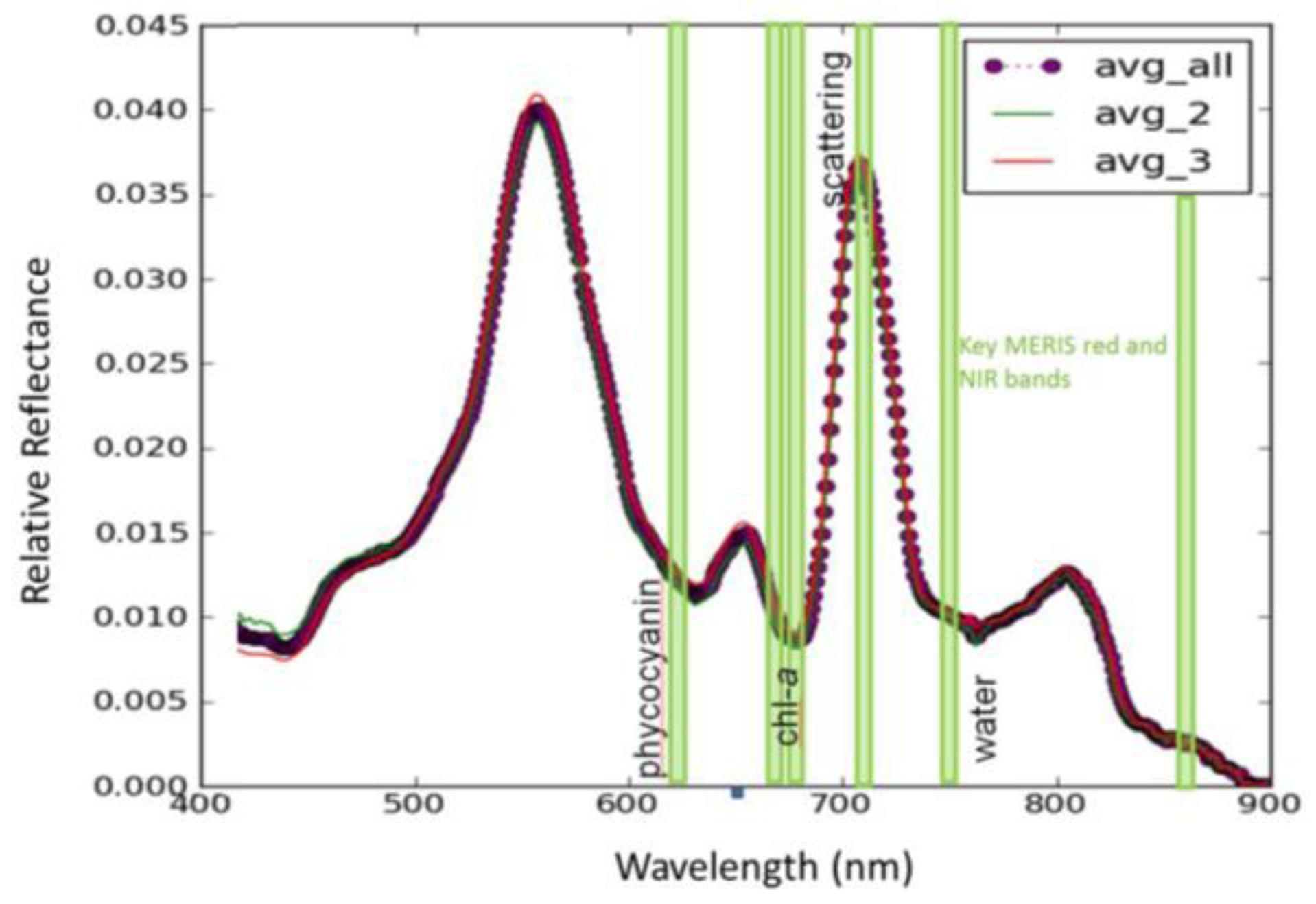
Figure 3.
Averaged reflectance spectra of an intense cyanobacterial (Microcystis) bloom over visible and near-infrared (NIR) wavelengths, with location of Sentinel-3/MERIS/OLCI red and NIR bands showing phycocyanin absorption at 620 nm, chlorophyll-a absorption at 670 nm and chlorophyll-a reflectance peak at 724 nm [27]. X-axis is wavelength in nanometers, and Y-axis is relative reflectance. Only a few of the existing satellite imaging systems can measure the depth of the approximately 620 nm phycocyanin absorption feature relative to other parts of the visible to near-infrared spectrum. Image via IEEE Earthzine: “Satellite Monitoring of Toxic Cyanobacteria for Public Health” https://earthzine.org/2014/03/26/satellite-monitoring-of-toxic-cyanobacteria-for-public-health/.
BGA algorithms based on the reflectance spectrum of phycocyanin should be better indicators of cyanobacteria than Chl-a algorithms because of their specificity, but are more difficult to adapt to existing satellite imaging systems due to much of the phycocyanin reflectance spectrum being masked by Chl-a and other pigments [11]. Only those imagers that sense a narrow absorption feature near 620 nm are well suited for the direct estimation of phycocyanin and BGA (Table 1). We have focused on relatively simple algorithms for BGA/PC estimation accordingly. Other water quality parameters such as Chl-a often co-occur and may co-vary with BGA and may be used as proxies for BGA in some water bodies [3,6,7,8,9,10,11,14,15,17,23,24,28,29,30].

Table 1.
Band wavelength ranges, centers and widths for original and synthetic satellite imagers. FWHM is Full Width Half Maximum.
Even with direct BGA estimation based on phycocyanin spectral features, not all species of cyanobacteria produce toxins and even the same species of BGA may or may not produce toxins depending upon environmental conditions. Therefore, remote sensing of algal blooms and especially BGA blooms is a first-cut technology that can “red flag” cyanobacterial blooms but cannot assess toxicity directly [24].
In this study we balance accuracy with portability across a variety of satellite imagers to counter frequent cloud cover issues during the humid temperate summers of southwest Ohio, and to create a practical first-cut capability for potential HAB monitoring. The target users for this technology are water quality managers of smaller inland water bodies less than a few km across. Given that no current remote sensing technology can actually detect the toxins in algal blooms [24], our operational goal is to find groups of imager/algorithm combinations that appear promising for the detection of algal blooms. Once a significant algal bloom is detected it will be necessary to collect water samples to evaluate toxicity. Therefore we are not concerned about detecting very low values of chlorophyll-a or phycocyanin nor are we concerned about saturation at high Chl-a/BGA values or differentiating high Chl-a/BGA values from surface algal scums for the purposes of this near-term warning and monitoring system. Characterizing Chl-a [6] and/or BGA/PC (this study) values as low, medium or high will be sufficient in this context of smaller inland water bodies in temperate climates like that of Ohio due to frequent summer cloud cover. Interpretation of low, medium or high will depend on the algorithm index and imager in a regional context. Regional water quality managers will then be able to use their experience in combination with field-based toxicity data to determine thresholds and appropriate responses to algal blooms.
Several studies have used high spectral resolution surface point and imaging spectroradiometers with numerous and narrow (“hyperspectral”) band configurations to collect reflectance signatures of BGA laden inland waters in order to formulate algorithms to estimate BGA values based on the phycocyanin reflectance signature [7,8,10,11,13,14,17,31,32]. We have favored simple algorithms for the reasons above. In several cases, we have followed the band choices of previous workers in simplified versions of their algorithms [7,8,10] or transferred their band choices to new or variants of existing algorithms [7,8,9,11,17].
Surface phytoplankton values are influenced by wind (mixing and drifting) as well as changes in the nutrient flux and water temperature, among other variables. Phytoplankton communities, in general, are dynamic on the scale of days and sometimes hours [29,30,31,32,33,34,35,36,37,38,39]. Moderate resolution satellites such as Landsat-8 can provide affordable sources of imagery for water quality monitoring in inland reservoirs [40]; however, their fixed revisit times, fixed observation angles and small constellations (usually a single satellite) limit their temporal resolution (e.g., 16 days for Landsat-8). It is therefore desirable to use a variety of low-cost sources of moderate spatial resolution satellite imagery from different satellites to increase temporal resolution and maximize the chances of successful image acquisition. Moderate resolution satellites such as Landsat-8, Sentinel-3/MERIS/OLCI, the Moderate Resolution Imaging Spectrometer (MODIS), and the new Sentinel-2 A&B constellation have a variety of both spatial resolutions and band configurations [33,34,35,36,37,38,39,40]. Not all satellite BGA/PC algorithms can be applied to all existing moderate resolution satellite imagers accordingly.
2. Methods
The methods used in this comparison of phycocyanin algorithms are similar to those of the companion study on chlorophyll-a [6]. This section is abbreviated accordingly. Our research used the following key datasets: airborne visible and near-infrared (VNIR) hyperspectral imagery of Harsha Lake and extensive, coincident surface spectral observations, laboratory measurements of water quality parameters and in situ water sensors. YSI BGA probe data were used to develop and calibrate a set of numerical algorithms for rapid and economical quantitative estimation of BGA values in this study.
2.1. Coincident Surface Observations of BGA
Twenty-seven established and new algorithms for BGA/PC estimation, either directly or via Chl-a proxy, were tested against the BGA/PC YSI probe (sonde) data for the real CASI aircraft hyperspectral imagery and for synthetic versions of several multispectral satellites. As stated above, our goal is the regional to local operational use of decades of previous work by others on reflectance algorithms for HAB detection. For this reason, we have focused our coincident surface observations on YSI BGA/PC relative fluorescence unit (BGA_PC_RFU) values to provide water quality managers with a rapid, affordable and common method for surface BGA/PC calibration for the most promising reflectance algorithms discussed below. This approach is adequate for our task because even BGA/PC concentrations (as opposed to BGA_PC_RFU values) are not a direct indicator of toxicity. Determination of toxicity requires at least limited and focused water sampling followed by laboratory analyses [5].
Given the variety of band center wavelengths and bandwidths for these different real and synthetic imagers, 184 variants of the initial 27 algorithm/imager combinations were created for this companion study in which we used the same aircraft imaging spectrometer dataset and field methods described in Beck et al. [6]. We then evaluated the initial set of Chl-a algorithms [6], several published BGA/PC algorithms as well as some new BGA/PC algorithms and their observed image-derived indices against (field/measured/observed) BGA estimates from in-situ fluorometry using a YSI brand BGA probe for measuring PC in the field and laboratory microscope-based BGA cell counts from water samples collected within 1 h of aircraft hyperspectral imager (imaging spectrometer) acquisition.
2.2. Atmospheric Correction of CASI Hyperspectral Aircraft Imagery
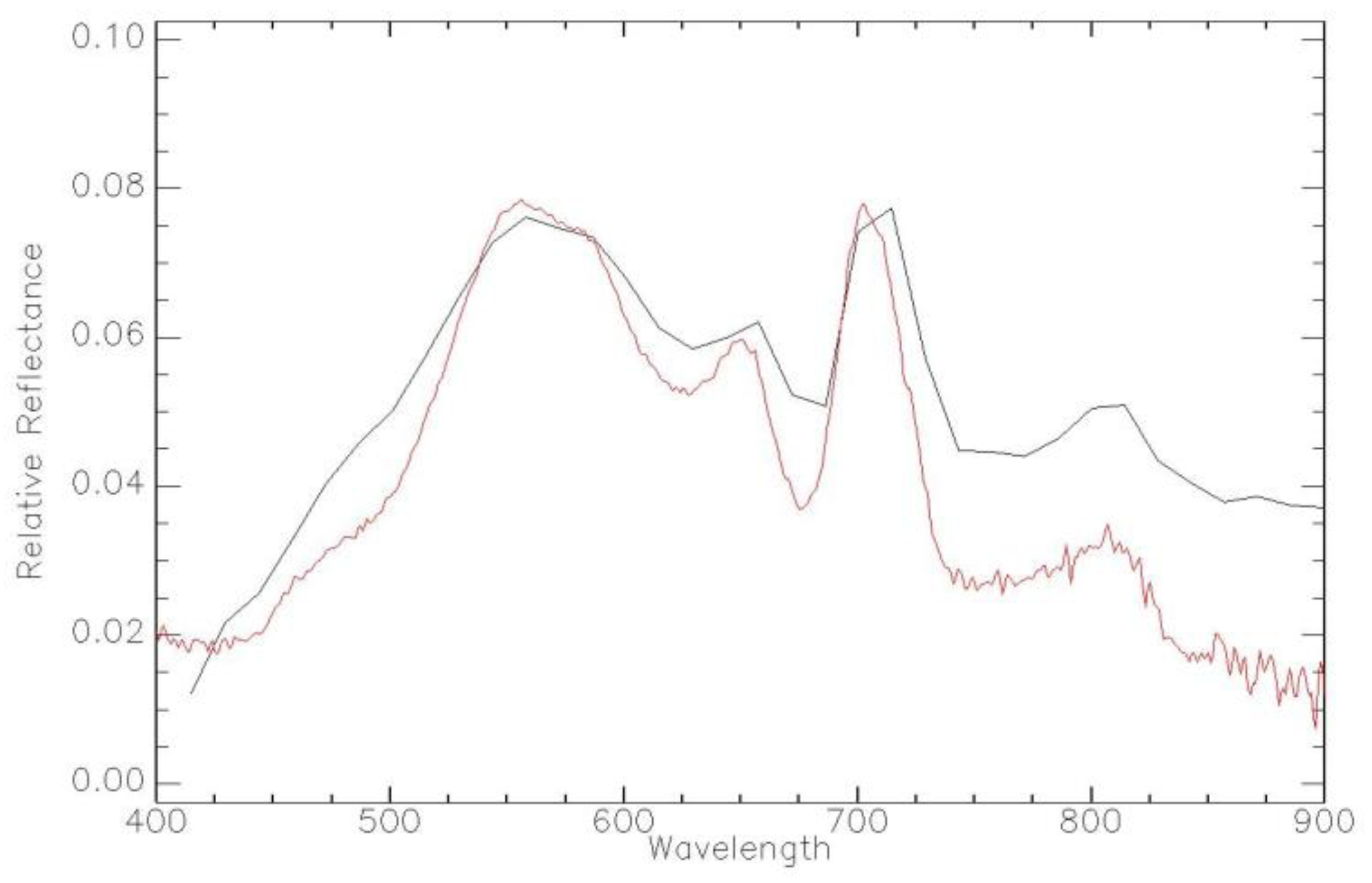
All of the synthetic imagery used for the following performance analysis with regard to the estimation of BGA is derived from VNIR CASI data atmospherically corrected to reflectance [6]. Atmospheric correction is usually incomplete, especially in regions of high humidity, nonetheless, we observed strong visual similarity of our pixel reflectance and Analytical Spectral Devices (ASD) reflectance spectra, very strong visual similarity of spatial pattern between image derived Chl-a indices and our coincident surface observations and strong (r2 > 0.6; p < 0.001) to very strong (r2 > 0.7; p < 0.001) observed vs. predicted Pearson’s r2 values depending on coincident surface observation type. The visual similarity of our surface and aircraft relative reflectance spectra is also confirmed statistically. For example, we averaged all 16 United States Army Corps of Engineers (USACE) surface ASD and USACE CASI (FLAASH) reflectance spectra from 16 locations from Harsha Lake and then normalized the CASI data to the ASD data in the Spectral Analysis and Management System (SAMS) at 550 nm in Figure 4 for comparison.
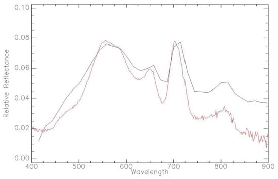
Figure 4.
Averaged Analytical Spectral Devices (ASD) surface relative reflectance spectra (red) vs. Averaged CASI reflectance spectra (n = 16) (black) for Harsha Lake with CASI data normalized to ASD at 550 nm. Wavelength in nm. They correspond well over the 425 and 865 nm wavelength range used in our study. One can even see a slight depression in the CASI spectra at 620 nm that corresponds to the phycocyanin absorption feature.
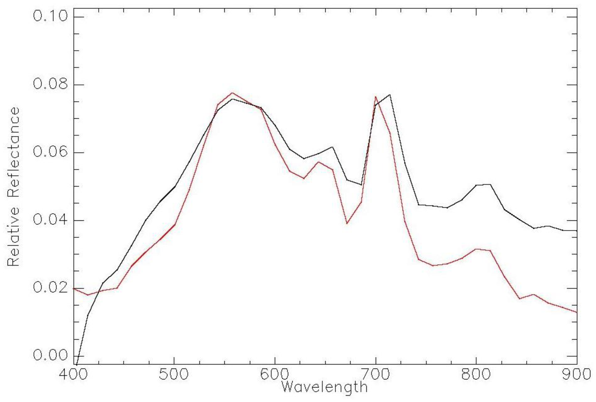
We then resampled the averaged ASD reflectance spectrum to the averaged CASI reflectance spectrum to obtain relative reflectance values at the same scale at the same wavelengths (Figure 5).
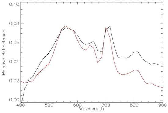
Figure 5.
Averaged ASD surface relative reflectance spectra (red) resampled to the same wavelengths as our CASI data vs. Averaged CASI reflectance spectra (n = 16) (black) for Harsha Lake with CASI data normalized to ASD at 550 nm. Wavelength in nm.
Our study used wavelengths from 425 to 865 nm (Table 2) so we created an observed vs. predicted (OP) Pearson’s regression (ASD surface vs. CASI aircraft relative reflectance) for all reflectance value pairs between those wavelengths. We verified this atmospheric correction by normalizing CASI to ASD spectroradiometer relative reflectance values at 550 nm at 16 locations and then evaluated their similarity with a linear regression of the relative reflectance value pairs for the 425 to 865 nm wavelengths used in this study with excellent results (Figure 6).
Table 2.
Band math and original specified wavelengths in nm for each algorithm used for blue-green algae/phycocyanin (BGA/PC) relative fluorescence unit (RFU) estimation at Harsha Lake. Float refers to floating point values of relative reflectance in the ENVI band math we used in this study at the specified wavelengths in nm from atmospherically corrected imagery. Float is not a variable; it is an IDL function used to prevent byte overflow errors during calculation. Asterisk after algorithm denotes design specifically for phycocyanin detection.
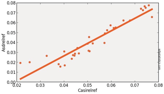
Figure 6.
Pearson’s test of linear correlation for ASD vs. CASI relative reflectance values at 32 wavelengths (n = 32). r2 = 0.89, p < 0.001, degrees of freedom = 30, slope = 1.265, intercept = −0.024.
Figure 5 and Figure 6 show some overestimation of reflectance by the atmospherically corrected CASI data, although the spectral shapes are similar. Therefore, the following algorithm/imager vs. coincident surface water observation regression results are for atmospherically corrected imagery for all of the real aircraft and synthetic satellite sensors considered below.
The atmospherically corrected (relative reflectance) CASI airborne hyperspectral imagery was upscaled to synthesize moderate resolution satellite data to develop specifications for a prototype multi-satellite monitoring system for HABs in our case study lake, Harsha Lake, in Southwest Ohio [6]. The band characteristics of our synthetic satellite imagers are summarized in Table 1. The original established algorithms, authors and band math with the original wavelength centers for Chl-a (indirect) and BGA/PC (direct) phycocyanin/BGA estimation algorithms are listed in Table 2. The algorithm/imager combinations and our 184 adaptations of the original algorithms to new wavelength centers for several synthetic satellite imagers are listed in Table S1. It is important to note that most of the existing algorithms were designed for different water bodies, including some CASE 1 water bodies [25] with different imagers. Imagers often have differing band centers, widths and spacing so the performance of the adapted algorithms here reflects our attempts at portability to new imagers in this circumstance only (a smaller temperate inland reservoir and perhaps some similar CASE 2 [25] waters) and does not reflect on the scientific talent of the original authors. Indeed, some established algorithms perform poorly with our narrow band real aircraft CASI data and better with spectral (and spatial) binning in our synthetic satellite data or vice-versa, as will be described below.
3. Results
Single-band output from the Band Math function in ENVI for each BGA algorithm (ENVI Band Math Field in Table 2 and Table S1) was point sampled using the coincident surface observation locations (Figure 2) to extract BGA index (image) values for comparison with measured YSI sonde BGA/PC relative fluorescence unit values (BGA_PC_RFU) collected within 1 h of the CASI overflight. Strong correlations (Pearson’s r2 > 0.6; p < 0.001) between image derived indices and dense coincident surface observations of BGA during this experiment indicate that Be162BsubPhy, SI052BDA, Be162B700sub601, Be16NDPhyI, Gi033BDA, Da052BDA, SM122BDA, Ku15PhyCI, MM092BDA, MI092BDA, Wy08CI, Zh10FLH, and MM12NDCI BGA algorithms worked well with CASI imagery. The Be162BsubPhy, SI052BDA, Am092Bsub, Be16NDPhyI, Mi092BDA, and MM12NDCI BGA algorithms worked well (Pearson’s r2 > 0.6; p < 0.001) with simulated WorldView-2 and -3, imagery; the Be162Bsub algorithm with simulated Sentinel-2 imagery; the Be16FLHviolet with simulated Landsat-8 imagery; and the MM092BDA, Be16NDPhyI, MM12NDCI, Go04MCI, Ku15PhyCI, Wy08CI, SI052BDA, Be162BsubPhy, and Hu103BDA BGA algorithms with simulated Sentinel-3/MERIS/OLCI imagery. The Be162BsubPhy algorithm was the most widely applicable BGA algorithm with good performance for CASI, WorldView-2 and -3, Sentinel-2 and MERIS-like imagery and limited performance with MODIS imagery. The Be16FLHviolet “greenness” algorithm yielded the best (although poor) BGA/PC estimates with simulated Landsat-8 imagery.
We also conducted an extensive survey of other water quality parameters in the lake at the time of acquisition in order to determine why some proxy indices such as Chl-a may also work with regard to BGA estimation. Details of our statistical treatment of the data are available in Beck et al. [6]. Type 1 (Pearson’s) r2 values were used to evaluate algorithm performance with raw index values vs. BGA/PC relative fluorescence units (BGA_PC_RFU) values measured with YSI BGA optical sondes in the water (Table S2) and as index values normalized to BGA values vs. BGA_PC_RFU values (Table S3) to facilitate comparison.
We used a critical p-value of 0.001 for all Pearson’s r Type 1 regression tests. Some researchers prefer Standard Error of Regression (Standard Error of Estimate or S) values to Type 1 (Pearson’s) r2 values so we have also included them for the top performing algorithms from Table S3 for comparison (Table 3). Other researchers prefer Type 2 regressions [48] to test correlations of observed vs. measured values [49] in natural systems. Therefore, we also applied the Type 2 geometric mean method of Peltzer [48] to BGA estimation at Harsha (East Fork) Lake with all results again normalized to calculated BGA values for top performing algorithms for each imager by Type 1 regression tests [17] (Table 4). A combined error budget for radiometry and multispectral image synthesis is presented in the chlorophyll-a companion paper [6].
Table 3.
Performance of Algorithms for BGA Estimation at Harsha (East Fork) Lake with all results normalized to calculated BGA values with additional Type 1 Regression tests for Standard Error of Regression (Standard Error of Estimate or S values) and associated statistics. Float refers to floating point values of relative reflectance in the ENVI band math we used in this study at the specified wavelengths in nm from atmospherically corrected imagery. Float is not a variable; it is an IDL function used to prevent byte overflow errors during calculation.
Table 4.
Performance of Algorithms for BGA Estimation at Harsha (East Fork) Lake with all results normalized to calculated BGA values with additional Type 2 Geometric Mean Tests for top performing algorithms by Type 1 Regression tests.
Examples of promising algorithms as applied to real CASI aircraft hyperspectral imagery and synthetic multispectral satellite imagery are discussed below.
3.1. CASI Imagery
We applied 27 algorithms in the form of 70 variants to the 1-m, 48-band CASI VNIR hyperspectral reflectance image mosaic (Tables S1, S2 and S4 and Figure 7). CASI has a narrow band capable of measuring the 620 nm phycocyanin absorption feature. The performance of each algorithm in Table 2 and Table 3 applied to the CASI reflectance imagery was then evaluated using 29 coincident surface observations for the sake of consistency with synthetic WorldView-2 and -3, Sentinel-2 and Landsat-8 imagery (other sub-30 m imagery). Simple subtraction, ratio-based and shape metric (second derivative) algorithms that include the 620 nm phycocyanin absorption feature and/or reflectance in the near-infrared suppress illumination variation well and had the best performance with regard to BGA estimation. In decreasing order of performance (Pearson’s r2), the CASIBe152BsubPhy, CASISI052BDA, CASIBe162B700sub601, CASIBe16NDPhyI, CASIGi033BDA, CASIDa052BDA, CASISM122BDA, CASIKu15PhyCI, CASIMM092BDA, CASIMi092BDA, CASIWy08CI, CASIZh10FLH, and CASIMM12NDCI algorithms worked well (Pearson’s r2 > 0.600) for BGA estimation with CASI imagery. Index imagery with raw and normalized index Type 1 (Pearson’s r) linear regressions are shown for the best performing algorithm (CASIBe152BsubPhy) in Figure 7.

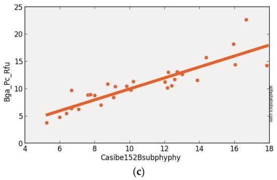
Figure 7.
Results of CASIBe152BsubPhy (715sub615) algorithm (this paper) as raw index values as applied to original CASI imagery with brighter pixels in the reservoir indicating higher BGA/PC values (a). Evaluation via observed (Y axis = BGA_PC_RFU) vs. predicted (calculated) raw CASIBe152BsubPhy (715sub615) index value with Pearson’s r2 (r2 = 0.776 p < 0.001, n = 29 to avoid shorelines) (b). Evaluation via observed (Y axis = BGA_PC_RFU) vs. normalized predicted (calculated) BGA values (CASIBe152BsubPhyPHY) with Pearson’s r2 (r2 = 0.776, p < 0.001, n = 29 to avoid shorelines) (c). Details of the synthetic bands and band math are available in Table 1 and Table 2, respectively.
Excellent results for several algorithms with CASI high resolution aircraft imagery for BGA_PC_RFU value estimation and their resulting index maps (Figure 7a) reveal considerable spatial heterogeneity at the 1 m scale in Harsha Lake at the time of aircraft image acquisition. This spatial heterogeneity of BGA/PC values in the imagery is supported by strong correlations with dense coincident surface observations (Figure 7b,c). Figure 5a also shows a strong correlation between the locations of the inflow from the East Fork of the Little Miami River in the NE corner of the image and the largest region of high BGA_PC_RFU values. In general the east basin of Harsha Lake has higher BGA/PC values than the west basin (Figure 7a). One can also see gyre-like structures associated with the dissipation of the BGA/PC-rich waters from east to west across the lake. The spatial heterogeneity displayed by the processed CASI images is masked to varying degrees in the coarser spatial resolution synthetic satellite data derived from this real CASI relative reflectance data as shown below. This masking of spatial heterogeneity in the east and west basins in coarse resolution satellite imagery also appears to exaggerate the contrast in BGA/PC values between the east and west basins of Harsha Lake. We view the high correlations of coincident surface observations with predicted BGA/PC values with coarse resolution synthetic MERIS/OLCI data presented below with some caution accordingly.
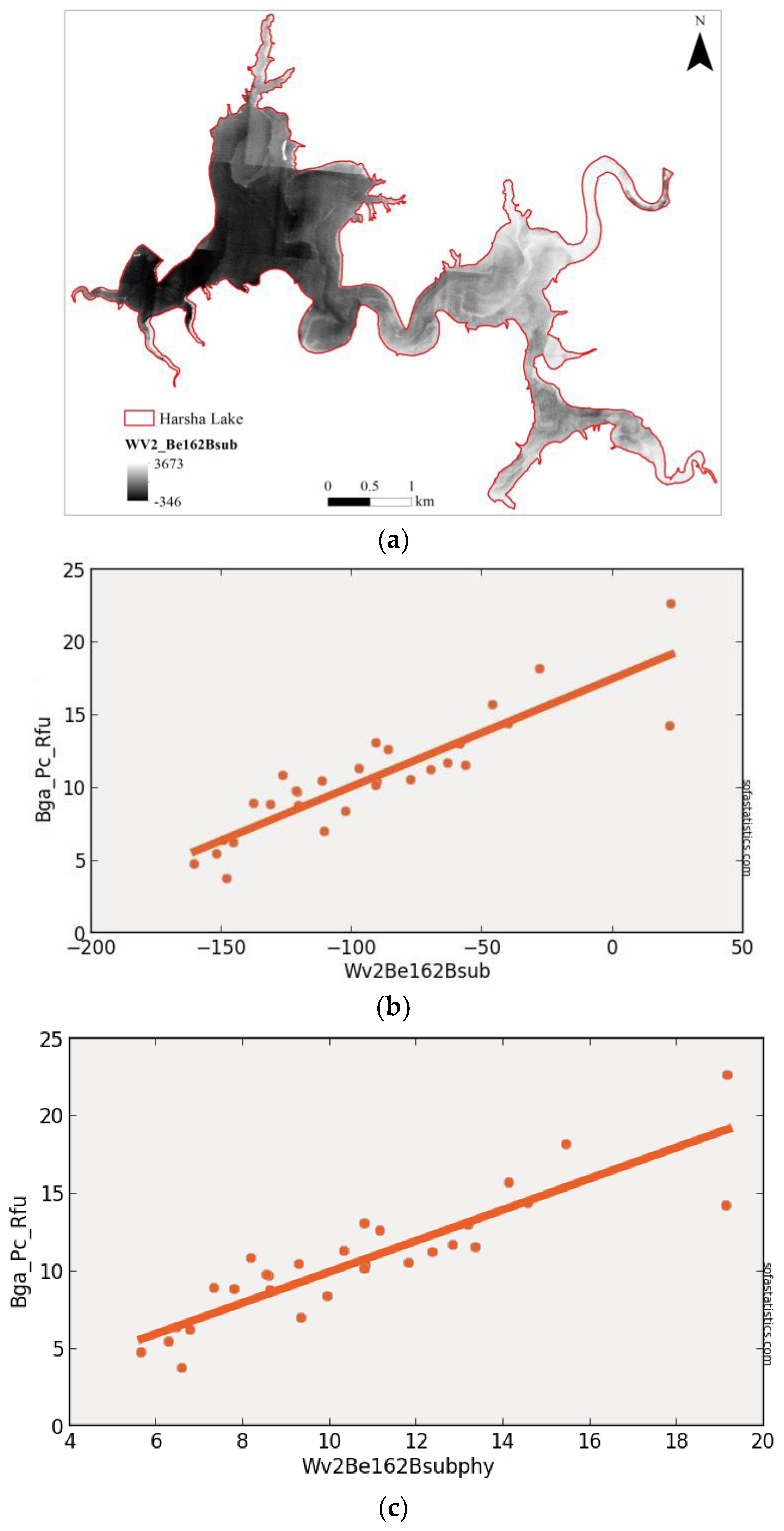
3.2. WorldView-2 (Synthetic)
We applied 11 existing and two new algorithms in the form of 25 variants to synthetic 1.8-m, WorldView-2 imagery to examine the degree of portability of some of the simpler algorithms between (synthetic) satellite imaging systems (Tables S1, S2 and S4 and Figure 8). WorldView-2 has a narrow band capable of measuring the 620 nm phycocyanin absorption feature. We also applied a new subtraction algorithm (Be162Bsub) and a new modified NDCI algorithm [32] (Be16NDPhyI) tuned to the 620 nm phycocyanin absorption feature. In decreasing order of performance, seven algorithms, WV2Be162Bsub, WV2SiO52BDA, WV2Am092Bsub, WV2Be16NDPhyI WV2Mi092BDA, and WV2MM12NDCI, had acceptable performance (Pearson’s r2 > 0.6; p < 0.001) with this sensor in this exercise (Figure 8). The performance of each algorithm in Table 2 and Table S1 applied to the synthetic WorldView-2 imagery was evaluated using 29 coincident surface observations (Table S2 and S4). As with CASI, simple subtraction and ratio-based algorithms that include the 620 nm phycocyanin absorption feature and/or reflectance in the near-infrared suppress illumination variation well and had the best performance with regard to BGA/PC value estimation. Index imagery with raw and normalized index Type 1 (Pearson’s r) linear regressions are shown for the best performing algorithm (WV2Be162Bsub) in Figure 8.
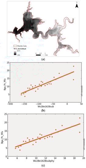
Figure 8.
Results of WV2Be162Bsub algorithm (this paper) as raw index values as applied to synthetic WorldView imagery with brighter pixels in the reservoir indicating higher BGA values (a). Evaluation via observed (Y axis = BGA_PC_RFU) vs. predicted (calculated) raw index value (WV2Be162Bsub) with Pearson’s r2 (r2 = 0.790, p < 0.001, n = 29 to avoid shorelines) (b). Evaluation via observed (Y axis = BGA_PC_RFU) vs. normalized predicted (calculated) BGA values (WV2Be162BsubPHY) with Pearson’s r2 (r2 = 0.790, p < 0.001, n = 29 to avoid shorelines) (c). Details of the synthetic bands and band math are available in Table 1 and Table 2, respectively.
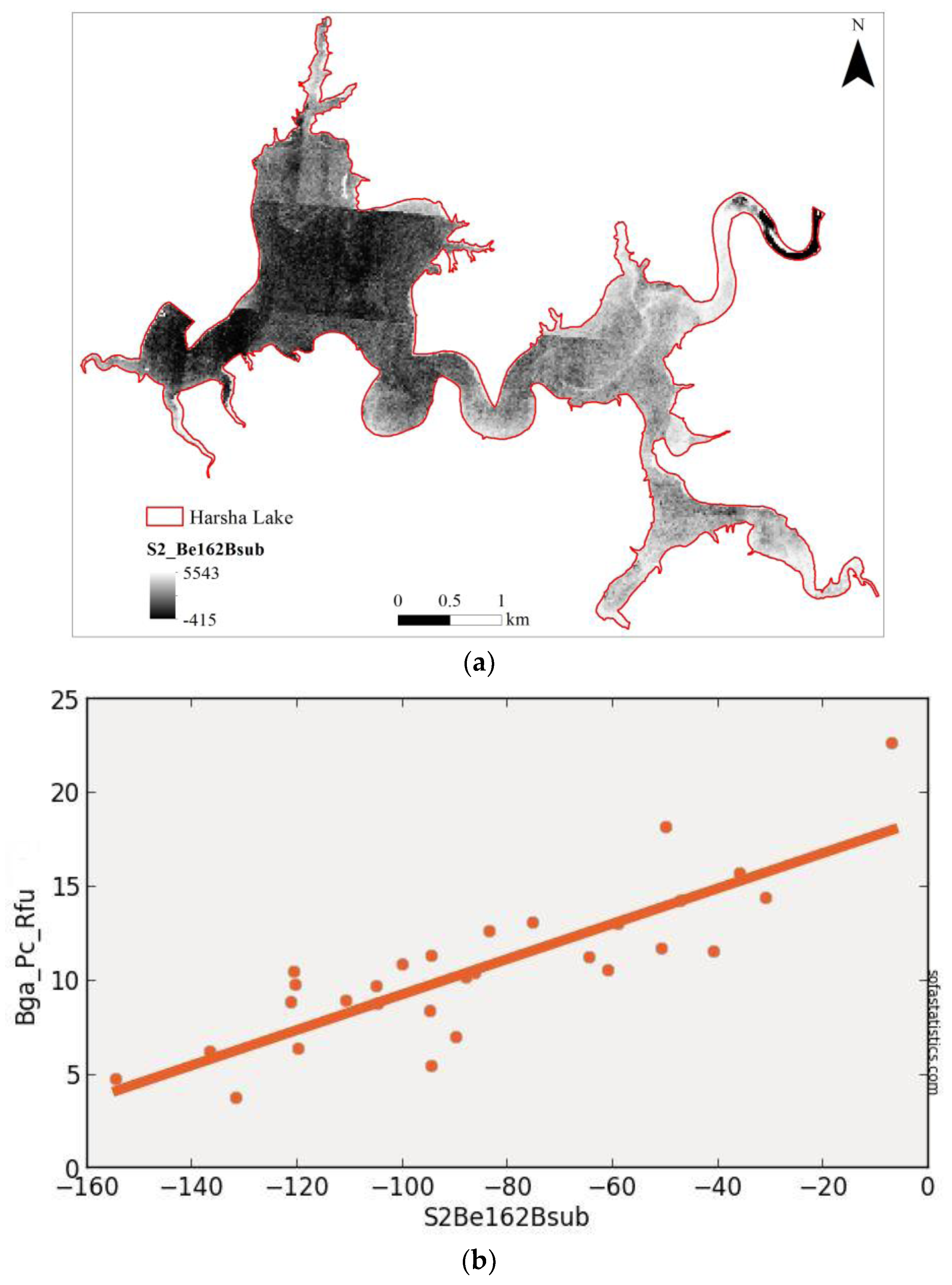
3.3. Sentinel-2 (Synthetic)
We applied eight existing and five new algorithms in the form of 23 variants to the 20-m, synthetic Sentinel-2 imagery. Sentinel-2 lacks a narrow band capable of measuring the 620 nm phycocyanin absorption feature. The performance of each algorithm in Table 2 and Table 3 applied to the synthetic Sentinel-2 imagery was evaluated using 29 coincident surface observations coincident surface observations chosen to avoid pixels that mixed land and water at 20 and 30 m spatial resolutions (Table S2 and S4). Six algorithms, S2Be162Bsub, S2SiO52BDA, S2Am092Bsub, S2MM12NDCI, S2Mi092BDA, and S2Be16NDPhyI, had acceptable performance (Pearson’s r2 > 0.6; p < 0.001) with this sensor in this experiment. The S2Be162Bsub, S2SiO52BDA, S2MM12NDCI, S2Mi092BDA, and S2Be16NDPhyI algorithms also appear to have good portability between CASI, WorldView-2/-3 and Sentinel-2 imagery (Table S2 and S4 and Figure 9). The strong performance of these algorithms with synthetic Sentinel-2 imagery and their wide swaths and dual constellation suggest that Sentinel-2 satellites will play a key role in future BGA monitoring systems for inland water quality. Index imagery with raw and normalized index Type 1 (Pearson’s r) linear regressions are shown for the best performing algorithm (S2Be162Bsub) in Figure 9.
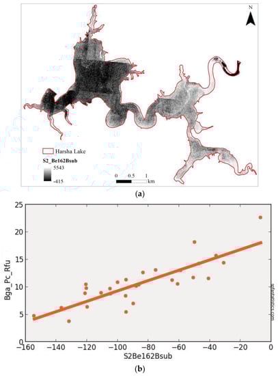

Figure 9.
Results of S2Be162Bsub algorithm (this paper) converted to BGA values as applied to synthetic Sentinel-2 imagery with brighter pixels in the reservoir indicating higher BGA values (a). Evaluation via observed (Y axis = BGA_PC_RFU) vs. predicted (calculated) raw index value (S2Be162Bsub) with Pearson’s r2 (r2 = 0.704, p < 0.001, n = 29 to avoid shorelines) (b). Evaluation via observed (Y axis = BGA_PC_RFU) vs. normalized predicted (calculated) BGA values (S2Be162BsubPHY) with Pearson’s r2 (r2 = 0.704, p value < 0.001, n = 29 to avoid shorelines) (c). The CASI data allowed the synthesis of Sentinel-2 bands 2 through 9 only. Details of the synthetic bands and band math are available in Table 1 and Table 2, respectively.
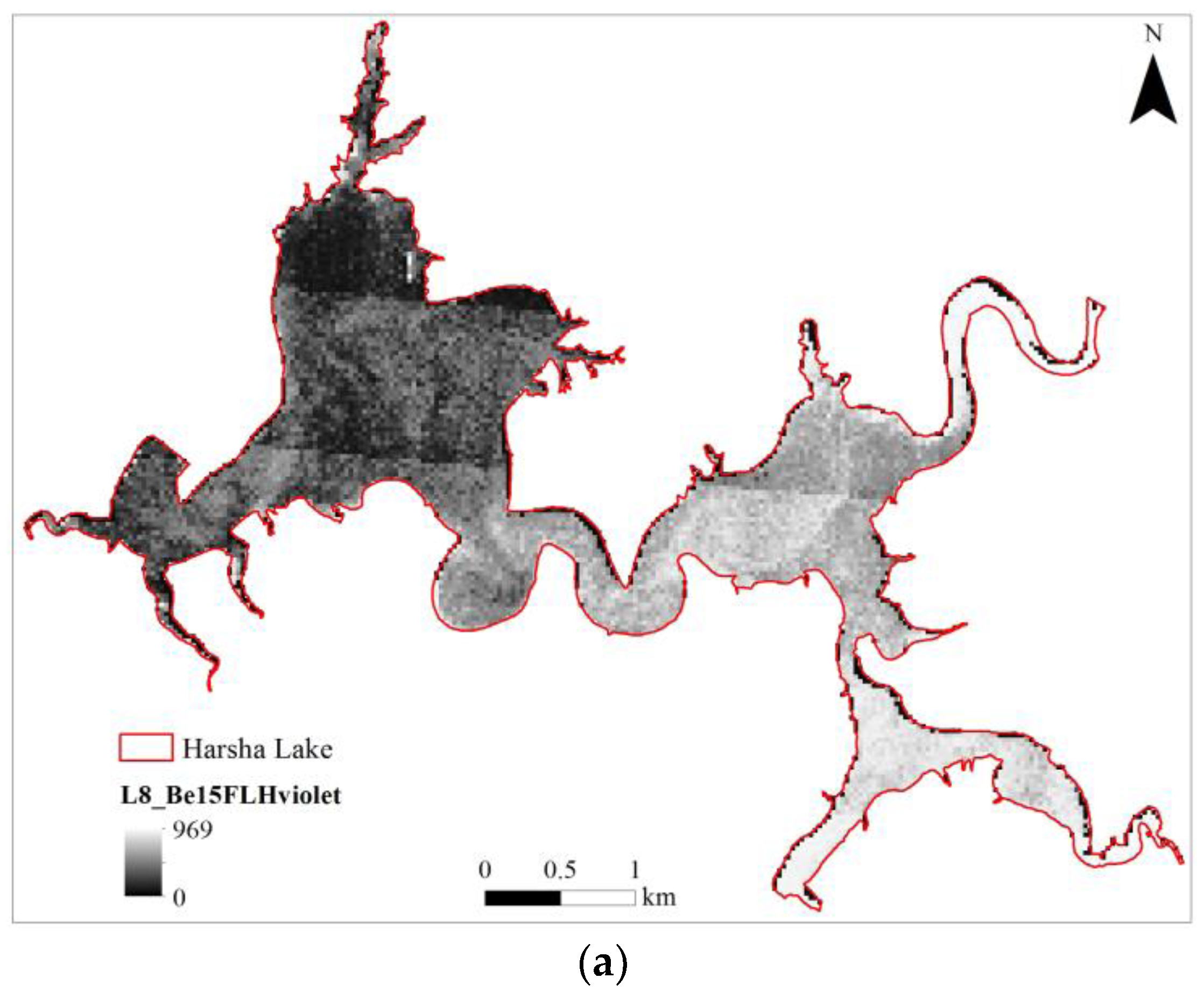
3.4. Landsat-8 (Synthetic)
We applied nine existing algorithms in the form of 17 variants to the 30-m, synthetic Landsat-8 imagery. Landsat-8 lacks a narrow band capable of measuring the 620 nm phycocyanin absorption feature. All of the algorithms applied here were indirect Chl-a proxy algorithms [6] accordingly. Moreover, the widths and positions of Landsat-8 bands also make the application of shape metrics for the Chl-a NIR reflectance peak feature infeasible and the application of some of the simple band ratio algorithms challenging (Table 2 and Table S1, Figure 10). The best performing algorithm was the green peak FLH Violet algorithm that incorporated the new ultra blue (“violet”) coastal band for this sensor in this experiment [6].

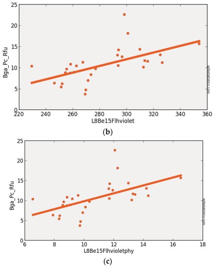
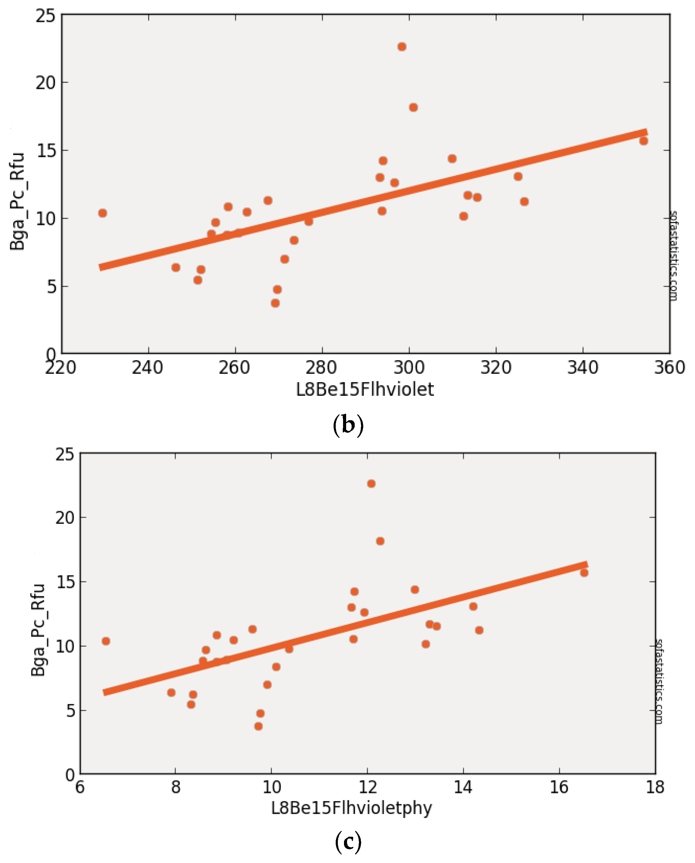
Figure 10.
Results of new FLH Violet algorithm [6] as raw index values as applied to synthetic Landsat 8 imagery with brighter pixels in the reservoir indicating higher BGA values (a). Evaluation via observed (Y axis = BGA_PC_RFU) vs. predicted (calculated) raw index value (L8Be15Flhviolet) with Pearson’s r2 (r2 = 0.339, p < 0.001, n = 29 to avoid shorelines) (b). Evaluation via observed (Y axis = BGA_PC_RFU) vs. normalized predicted (calculated) BGA values (L8_FlhvioletPHY) with Pearson’s r2 (r2 = 0.339, p < 0.001, n = 29 to avoid shorelines) (c). Details of the synthetic bands and band math are available in Table 1 and Table 2, respectively.
None of the simple spectrally-oriented semi-analytical algorithms (based at least in part on known spectral features associated with known water quality parameters) considered here had acceptable performance (Pearson’s r2 > 0.6; p < 0.001) with regard to BGA estimation with Landsat-8 in this exercise due to its design for land vegetation (Chl-a) rather than BGA/PC in water. Index imagery with raw and normalized index Type 1 (Pearson’s r) linear regressions are shown for the best performing algorithm (L8Be15Flhviolet) in Figure 10. Local empirical algorithms based on other water quality parameters such as Chl-a and turbidity with local calibration and validation are required for use with Landsat-8 for reliable BGA estimation because Landsat-8 cannot sense the 620 nm phycocyanin absorption feature [22].
3.5. MODIS (Synthetic)
We applied three existing algorithms (NDCI, 2BDA and Am092Bsub) in the form of six variants to synthetic MODIS bands 1 and 2 [43] for BGA estimation with limited success (Tables S1, S2 and S4, Figure 11). None of the spectrally-oriented semi-analytical algorithms considered here had acceptable performance (Pearson’s r2 > 0.6; p < 0.001) with regard to BGA estimation with this sensor in this experiment due to the wide MODIS bands. While MODIS could be a part of operational monitoring systems, its wide bands and coarse spatial resolution suggest that it will have limited value in operational monitoring systems for inland water quality, especially for smaller water bodies less than a few kilometers across. MODIS also lacks a narrow band capable of measuring the 620 nm phycocyanin absorption feature [50].
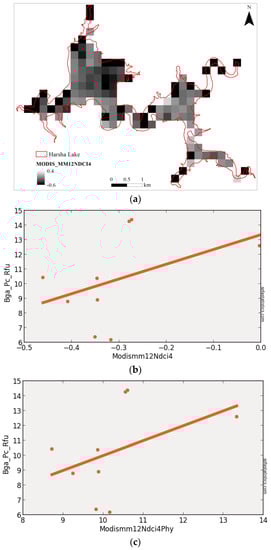
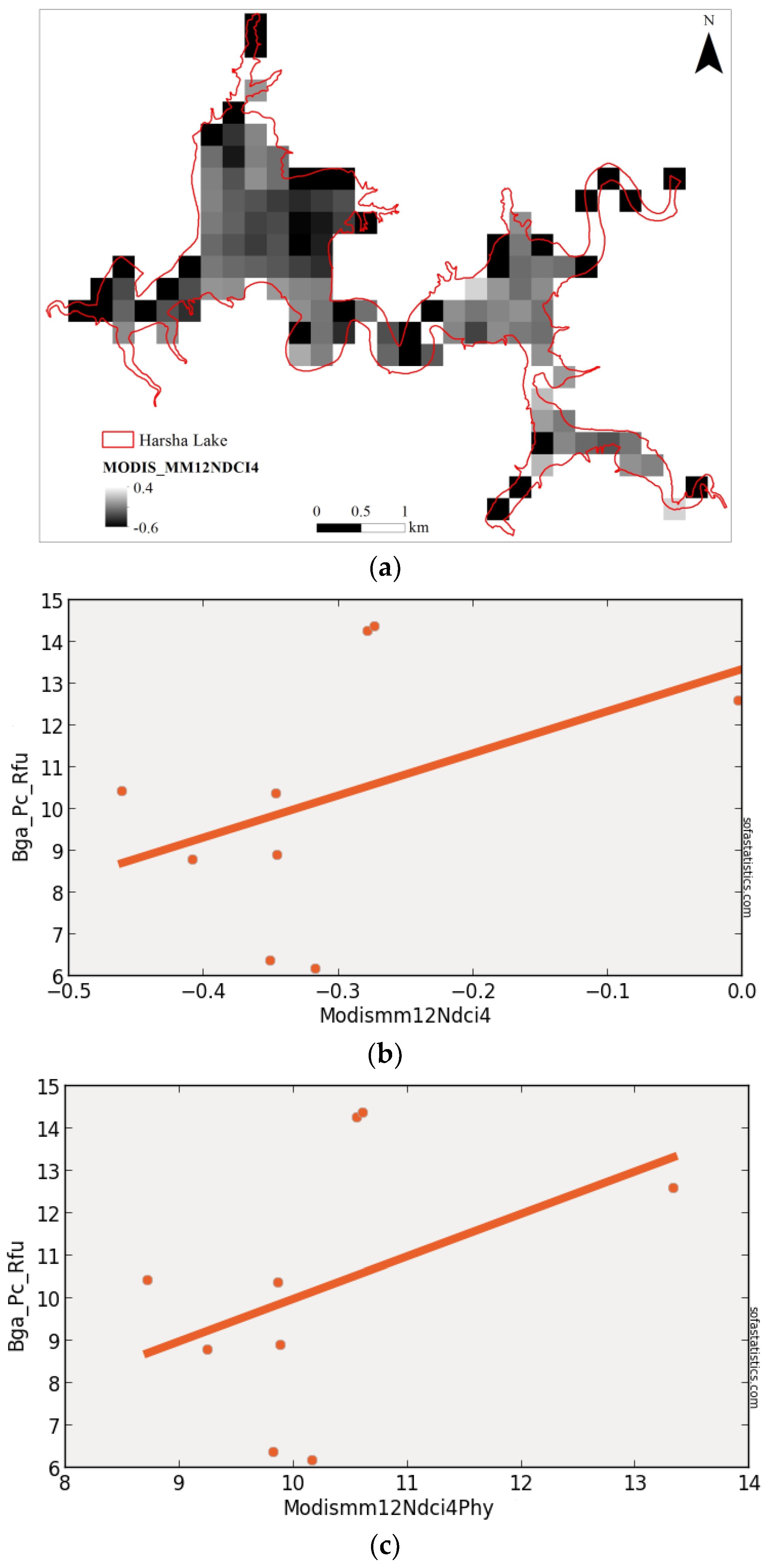
Figure 11.
Results of MODISMM12NDCI4 algorithm [32] converted to BGA values as applied to synthetic MODIS imagery with brighter pixels in the reservoir indicating higher BGA values (a). Evaluation as raw index values as applied to synthetic MODIS imagery and its evaluation via observed (Y axis = BGA_PC_RFU) vs. predicted (calculated) raw index value (MODISMM12NDCI4) with Pearson’s r2 (r2 = 0.183, p = 0.126, n = 9 due to large pixels) (b). Evaluation via observed (Y axis = BGA_PC_RFU) vs. normalized predicted (calculated) BGA values (MODISMM12NDCI4PHY) with Pearson’s r2 (r2 = 0.183, p = 0.126, n = 9 due to large pixels) (c). Details of the synthetic bands and band math are available in Table 1 and Table 2, respectively.
The performance of each algorithm in Table 2 and Table S1 applied to the synthetic MODIS imagery was evaluated using nine coincident surface observations. These nine points were chosen to avoid pixels that mixed land and water at 250 and 300 m spatial resolutions. MODIS bands 1 and 2 were simulated with the CASI data at 250 m spatial resolution to facilitate comparison of algorithm performance. MODIS bands 1 and 2 are commonly available at the 250 m spatial resolution and are part of the better performing algorithm (NDCI). This suggests that MODIS NDCI may have some modest utility with regard to BGA estimation and algal bloom monitoring in some larger inland water bodies. The large pixel sizes associated with MODIS make it more appropriate for relatively large water bodies using other water quality parameters such as Chl-a or turbidity as proxies for BGA/PC. MODIS imagery will also require severe masking to avoid shorelines (mixed land and water pixels) (Figure 9a). Index imagery with raw and normalized index Type 1 (Pearson’s r) linear regressions are shown for the best performing algorithm (MODISMM12NDCI4) in Figure 11.
3.6. MERIS (Synthetic)
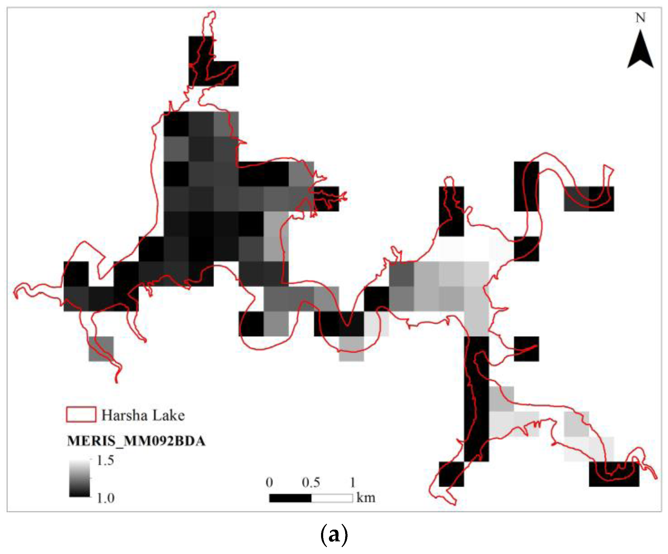
We applied the 13 existing and four new algorithms in the form of 35 variants for BGA estimation to synthetic Sentinel-3/MERIS/OLCI data for Harsha Lake with limited success (Tables S1, S2 and S4, Figure 12) before severe masking (Figure 12a). MERIS has a narrow band capable of measuring the 620 nm phycocyanin absorption feature. Ten of the BGA (direct) and Chl-a (indirect or proxy) spectrally-oriented semi-analytical algorithms considered here had acceptable performance (Pearson’s r2 > 0.6; p < 0.001) when tested against in situ YSI BGA probe data (BGA_PC_RFU) with this sensor in this experiment after severe masking. In order of decreasing performance, the MERISMM092BDA, MERISBe16NDPhyI, MERISMM12NDCI, MERISGo04MCI, MERISWy08CI and MERISKu15PhyCI, MERISSi052BDA, MERISBe162Bsub, MERISHu103BDA, and MERISMM143BDAopt algorithms all estimated BGA well in this exercise. We agree that MERIS/OLCI can be a part of operational water quality monitoring systems [20]. However, high-spatial resolution CASI data show that there was significant spatial heterogeneity in the values of BGA on a scale much finer than either Sentinel-3/MERIS/OLCI (300 m) or MODIS (250 m) pixels. Index imagery with raw and normalized index Type 1 (Pearson’s r) linear regressions are shown for the best performing algorithm (MERISMMO92BDA) in Figure 12.
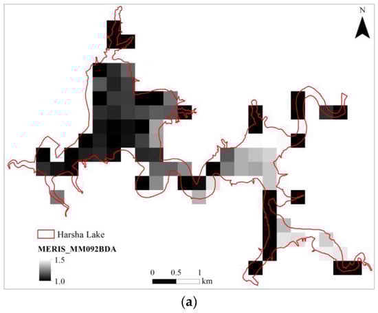
Figure 12.
Results of MERISMM092BDA algorithm (Mishra and Mishra, 2009) as raw BGA index values as applied to synthetic MERIS imagery with brighter pixels in the reservoir indicating higher BGA values (a). Evaluation via observed (Y axis = BGA_PC_RFU) vs. predicted (calculated) raw BGA index values (MERISMM092BDA) values with Pearson’s r2 (r2 = 0.863, p < 0.001, n = 9 due to large pixels) (b). Evaluation via observed (Y axis = BGA_PC_RFU) vs. normalized predicted (calculated) BGA (MERISMM092BDA) values with Pearson’s r2 (r2 = 0.863, p < 0.001, n = 9 due to large pixels) (c). Details of the synthetic bands and band math are available in Table 1 and Table 2, respectively.
4. Discussion
The focus of this study is on simple, portable, semi-analytical algorithms based on the phycocyanin and Chl-a spectral signatures. CASI, WorldView and MERIS are capable of sensing the narrow 620 nm phycocyanin absorption feature (Figure 1, Table 1). Algorithms specifically tuned to this phycocyanin feature had the best performance for 1 m CASI imagery (CASIBe152BsubPhy, r2 = 0.776) and 1.8 m WorldView imagery (WV2Be162Bsub, r2 = 0.790) and the second best for 300 m MERIS imagery (MERISBe16NDPhyI, r2 = 0.852) (Table S4). An indirect BGA index algorithm, MERISMM092BDA (r2 = 0.863), designed to measure Chl-a had the best performance with regard to BGA estimation with simulated MERIS/OLCI imagery.
Wheeler et al. [30] observed similar results for MERIS in Lake Champlain, New York, USA, with a stronger correlation of BGA to NIR reflectance than 620 nm absorption. They ascribed this result to non-linear absorption at 620 nm, spectral interference of Chl and other pigments with the 620 nm feature, due in part to surface scums, and temporal/environmental differences in phycocyanin absorption efficiency. Our results suggest that the large pixel sizes of MERIS may contribute to the masking of the 620 nm phycocyanin absorption feature, although the phycocyanin-tuned MERISBe16NDPhyI algorithm still had excellent performance (r2 = 0.852) probably due to the strong algal and turbidity contrasts between the eastern and western basins of Harsha Lake at the time of aircraft image acquisition. In addition, MERIS does not capture the spatial variation observed in higher resolution imagery discussed above accordingly [6]. We conclude that phycocyanin specific algorithms with strong performance are available for CASI, WorldView and MERIS-like imagers.
In contrast, Sentinel-2, Landsat-8 and MODIS are not capable of sensing the narrow 620 nm phycocyanin absorption feature (Figure 1, Table 1). We relied on Chl-a proxy algorithms summarized in [6] for BGA estimation with these imagers accordingly. The best performing Chl-a proxy algorithms for BGA were S2Be16Bsub for Sentinel-2 (r2 = 0.704), L8Be15Flhviolet for Landsat-8 (r2 = 0.339) and MODISMMNDCI12 for MODIS (r2 = 0.183). The strong performance of Sentinel-2 for BGA estimation via the S2Be16Bsub Chl-a algorithm makes it a valuable component for cyanobacterial monitoring in at least some inland water bodies similar to Harsha Lake. The poor performance of these semi-analytical Chl-a proxy algorithms for BGA estimation with Landsat-8 and MODIS mirrors their poor performance for Chl-a estimation due to their wide bands relative to distinctive parts of the Chl-a spectral signature in water [6]. Indirect empirical local algorithms based on one or several other co-varying water quality parameters may be necessary for Landsat-8 and MODIS algorithms accordingly and will require local tuning.
Ogashawara et al. [14] completed a performance review of reflectance based algorithms for predicting phycocyanin values in waters with both field and laboratory fluorometry. For this study we used field-based fluorometery using a calibrated YSI BGA probe. Despite our differences in approaches (surface remote sensing reflectance (Rrs) vs. aircraft relative reflectance) our results are remarkably similar. Ogashawara et al. [14] simulated Hyperion, CHRIS and HyspIRI narrow band imager data from their surface spectroradiometer data. They found the SI05, MM09, and MI09 algorithms all performed well (strong r2 values with modest RMSE values) with more modest results for the SC00 (SY00 in our study) [47] algorithm in their study. Our real calibrated aircraft relative reflectance based imagery showed the same pattern (Table S4). In fact, we found only one simple subtraction (Be162BsubPhy715sub615) algorithm that exceeds the performance of the simplified Simis algorithm [7] in our study. This simple subtraction algorithm leverages the band choices of Mishra et al. [11] for minimizing the Chl-a spectral overlap with that of the 620 nm phycocyanin absorption feature in their MI09 band ratio algorithm.
The strong performance of our simple subtraction algorithm in this particular “snap-shot” study with real narrow band CASI data may not hold for time-series imagery with illumination variation between dates of acquisition. Like Mishra et al. [11] we expect their MI09 ratio-based algorithm (and other band ratio and shape metric algorithms) to be more robust across time-series imagery because they inherently damp variations in illumination. In addition, similar to Mishra et al. [11], we used the simplified version of the Simis et al. [7] algorithm because we are trying to evaluate the portability of relatively simple algorithms between narrow, moderate and broad band satellite imagers [6], some of which have relatively limited band choices in order to create meta-constellations of current and near-term imagers for operational algal bloom monitoring. The performance of these algorithms with real imagers will vary due to differences in their on-orbit radiometry and for other water bodies due to variable values of BGA/PC and co-occurring water quality parameters including those described below.
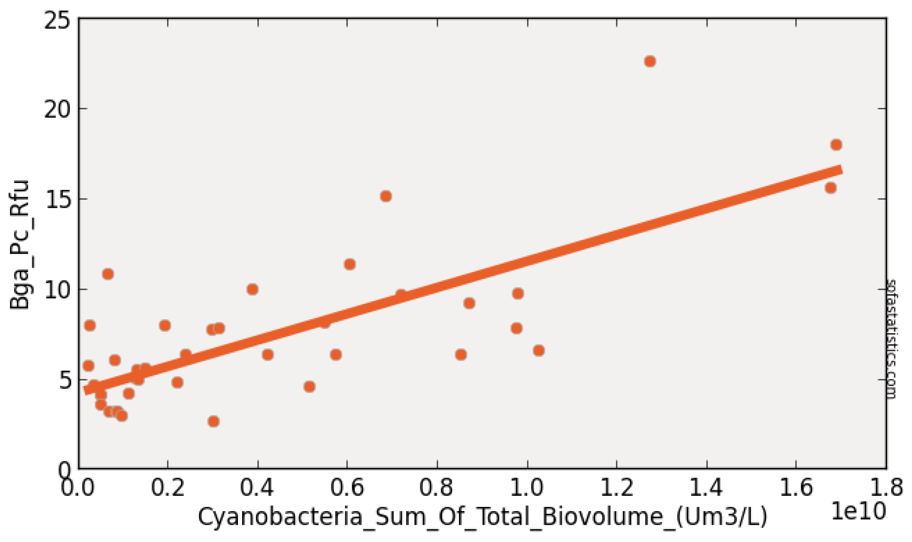
This study measured 41 water quality parameters (Table 5) at each of the 44 coincident surface observation sites during the hyperspectral overpass used to construct the coincident synthetic imagery for the satellite imaging systems considered above. These data helped to determine when and why some proxy algorithms such as those for Chl-a also work for BGA estimation. Of primary importance was quantifying the output of our YSI BGA fluorescence probes which recorded in BGA phycocyanin (PC) relative fluorescence units (BGA_PC_RFU) vs. total laboratory BGA cell counts (Figure 13). A comparison of these optical sonde BGA values (BGA-PC-RFU) vs. laboratory determined Cyanobacterial Sum of Total Biovolume (CSTB) values measured on the same day resulted in Pearson’s r2 = 0.757 with p < 0.001 and n = 39 (Figure 13). We are confident in the validity of using optical sonde BGA_PC_RFU values as the basis for our coincident BGA surface observations accordingly.
Table 5.
Water Quality Parameters Investigated for covariation with BGA.
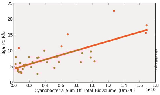
Figure 13.
Comparison of optical sonde BGA values (Bga-PC-RFU) vs. laboratory determined Cyanobacterial Sum of Total Biovolume values measured in Harsha and a nearby reservoir on the same days with Pearson’s r2 (r2 = 0.757, p < 0.001, n = 39).
Our normalized phycocyanin index values for the best performing algorithms for all imagers except MODIS allow us to predict phycocyanin values (BGA_PC_RFU) and in turn cyanobacterial sum of total biovolume (CSTB). For example if we were to determine that a CASI pixel has an estimated normalized index value of 12 (Figure 7c) this would correspond to a BGA_PC_RFU value of 12 as well. This BGA_PC_RFU value of 12 would in turn correspond with a CSTB value of approximately 1.2 µm3/L. One can make similar phycocyanin value estimates with WorldView-2 (Figure 8c), Sentinel-2 (Figure 9c), Landsat-8 (Figure 10c), and perhaps Sentinel-3/MERIS/OLCI (Figure 11c) and then CSTB estimates from Figure 13, respectively. We expect slopes and intercepts for normalized phycocyanin index values for the best performing algorithms derived from real WorldView-2, Sentinel-2, Landsat-8 (Figure 10c), and perhaps Sentinel-3/MERIS/OLCI reflectance imagery to differ somewhat from the synthetic results here. Once we have calibrated the time-series imagery from these imagers for the most promising algorithms identified here we will be able to make similar phycocyanin values and CSTB estimates for real satellite imagery.
Operational use of this method for estimating phycocyanin values (BGA_PC_RFU) and CSTB will be facilitated by the use of multiple satellite imaging platforms that will improve revisit times and help to alleviate summer cloud cover which limits the utility of single satellite HAB monitoring systems. For example cloud free images of Harsha Lake from Landsat-8 are available for perhaps 1 out of 4 overpasses. We hope to improve our temporal resolution by using the technique described above to approximately every two weeks by using Landsat-8 in combination with Sentinel-2a and -2b at a minimum. We will augment this coverage with WorldView-2 and -3 imagery when it is available to us. Larger water bodies should be able to use Sentinel-3/MERIS/OLCI imagery as well.
Our results show that several other water quality parameters were also correlated with BGA_PC_RFU values in Harsha reservoir at the time of hyperspectral image acquisition (Table 6). Thirteen water quality parameters had Pearson’s r2 values greater than 0.500. They were, in order of decreasing correlation, Turbidity (NTU) (r2 = 0.852), total suspended solids (TSS) (r2 = 0.789), total phosphorous (TP) (r2 = 0.724), particulate phosphorous (PP) (r2 = 0.697), volatile suspended solids (VSS) (r2 = 0.666), dissolved reactive phosphorous (DRP) (r2 = 0.661), total nitrogen (TN) (r2 = 0.656), Chlorophyll as concentration and as RFU (r2 = 0.651 and 0.640, respectively), total dissolved phosphorous (TDP) (r2 = 0.610), particulate nitrogen (PN) (r2 = 0.591), bicarbonate (HCO3-) (r2 = 0.551) and alkalinity as mg of CaCO3 (r2 = 0.542) (Table 5 and Table 6). Of these parameters, only Turbidity (NTU), TSS, VSS, and CHL, are spectrally active. Nonetheless, their strong co-variance with spectrally inactive water constituents explains why local empirical regressions against band reflectance values may be used to locally estimate a number of water quality parameters after local calibration [14,23,30] although their portability may be limited.
Table 6.
Correlation of Water Quality Parameters Investigated with BGA_PC_RFU as measured by Pearson’s r test.
In summary, there are several excellent semi-analytical spectrally based algorithm/imager combinations capable of estimating BGA values and cyanobacterial total volumes in smaller inland water bodies either directly via the phycocyanin signature with CASI, WorldView-2/-3, and Sentinel-3/MERIS/OLCI (Table S4) or indirectly via the Chl-a signature with Sentinel-2 and to a lesser extent Landsat-8 [6].
5. Uncertainties, Errors and Accuracies
Our Chl-a companion study [6] included an error budget for the radiometry of our real aircraft and synthetic satellite imagery that indicated radiometric uncertainties on the order of 200%. Similarly, our field spectra could have radiometric uncertainties on the order 800% based on previous sun glint and wave studies [51]. Nonetheless, the very strong performance of several well established BGA and Chl-a algorithms with our atmospherically corrected hyperspectral aircraft imagery suggests that our methods were more than adequate for our “red flag” early warning purposes. As noted above, we are also cautious about the very strong performance of MERIS in this study. Its extraordinary performance may be partially due to the high contrast in BGA values between the east and west basins of Harsha Lake at the time of the experiment. We are also cautious with regard to the very strong performance of the simple BGA subtraction algorithms we used and suspect that other algorithms such as the Mishra family of ratio algorithms may be more appropriate for time-series imagery in operational settings. For these reasons, we expect the algorithm performance rankings to differ somewhat with real imagery and have identified groups of promising imager/algorithm combinations accordingly (Tables S2 and S3). Nonetheless, we are confident of our overall results given the very strong performance of many well established BGA and Chl-a algorithms with our dense, nearly coincident surface observations.
6. Conclusions
This study used atmospherically corrected high-spatial and high-spectral resolution VNIR CASI hyperspectral imagery to construct synthetic WorldView-2, Sentinel-2, Landsat-8, MODIS and Sentinel-3/MERIS/OLCI image datasets with dense coincident surface observations in the form of in situ water quality sonde and laboratory measurements to evaluate the performance of reflectance algorithms for estimating BGA values in a 8.9 km2 temperate inland reservoir. The study focused on currently operational and near-future imaging satellite constellations that may be suitable contributors to an operational water quality monitoring system for smaller inland reservoirs, lakes and rivers.
6.1. Best Performing Imager/Algorithm Combinations for BGA Estimation
We found that several established algorithms for the estimation of BGA values performed well (Pearson’s r2 > 0.6; p < 0.001) for most of the real aircraft and synthetic satellite datasets considered here. The Be162BsubPhy, SI052BDA, Be162B700sub601, Be16NDPhyI, Gi033BDA, Da052BDA, SM122BDA, Ku15PhyCI, MM092BDA, MI092BDA, Wy08CI, Zh10FLH, and MM12NDCI BGA algorithms worked well with CASI imagery. The Be162BsubPhy, SI052BDA, Am092Bsub, Be16NDPhyI, Mi092BDA, and MM12NDCI BGA algorithms worked well with WorldView-2 and -3; the Be162Bsub algorithm with Sentinel-2; and the MM092BDA, Be16NDPhyI, MM12NDCI, Go04MCI, Ku15PhyCI, Wy08CI, SI052BDA, Be162BsubPhy, and Hu103BDA BGA algorithms with MERIS-like imagery. Be162BsubPhy was the most widely applicable BGA algorithm (Table S4). The Be16FLHviolet “greenness” algorithm yielded the best (albeit poor) BGA estimates with simulated Landsat-8 imagery.
Algorithm/imager combinations listed in the preceding paragraph that include the phycocyanin reflectance minimum at 620 nm had slightly better performance with regard to BGA estimation than Chl-a algorithms for CASI and WorldView-2 and were only slightly less effective than Chl-a algorithms for Sentinel-3/MERIS/OLCI as predicted by Simis et al. [7] and Mishra et al. [11] (Table S4). For imagers without a narrow band at 620 nm, we used Chl-a proxy algorithms to estimate BGA with good results for simulated Sentinel-2 and poor results for simulated Landsat-8 and MODIS for this water body at the time of hyperspectral image acquisition.
6.2. Portability of Algorithms between Imagers
The simple phycocyanin spectrum-based, semi-analytical Be162Bsub subtraction algorithms had the highest portability between the CASI, WorldView-2 and MERIS-like imaging systems. Other simple band ratio-based algorithms also suppress illumination variation between scenes and estimate BGA values well after imager and environment specific calibration (Table S4). This is especially effective when these simple subtraction and band ratio algorithms are applied to imagers with relatively narrow bands that capture the 620 nm phycocyanin reflectance minimum (Si052BDA for CASI, WorldView and MERIS) or near-infrared/red Chl-a reflectance contrast (MM092BDA also for MERIS). The normalized difference phycocyanin index (Be16NDPhyI for CASI, WorldView and MERIS) and normalized difference chlorophyll index [32] (MMNDCI12 for CASI, WorldView, Sentinel-2, and MERIS) algorithms also performed well with regard to BGA estimation (Table S4). Landsat-8 requires an alternative algorithm such the Chl-a “greenness” FLH Violet algorithm [6]. MERIS and MODIS do not capture the spatial heterogeneity in BGA observed in this study due to their large pixels. MODIS has wide bands that do not target the “veg edge” or BGA absorption feature well and has low performance accordingly (Tables S2 and S4) although it may be useful with NDCI for larger water bodies.
6.3. Implications for Operational BGA Monitoring with Existing and Near-Future Satellites
For imagers with appropriate bandwidths and positions relative to the BGA phycocyanin reflectance signature and pixel sizes appropriate for smaller inland water bodies less than a few km across, simple algorithms that subtract or ratio bands and therefore inherently normalize reflectance performed well and appear to be relatively portable between most satellite imaging systems for the estimation of BGA in smaller inland water bodies. Therefore, near-term steps toward operational water quality monitoring systems for inland water bodies smaller than a few kilometers across should focus on Sentinel-2 A and B and to a lesser extent Landsat-8 with augmentation from WorldView-2 and -3 or hyperspectral imagery when required. Good performance of both BGA and Chl-a algorithms for BGA estimation suggests that early efforts to operationalize regional algal monitoring can use whichever set of algorithms are most appropriate for the sources of imagery at hand (Sentinel-2/3, WorldView-2/3 and to a lesser extent Landsat-8). Sentinel-3/MERIS/OLCI may also be useful for heavily masked time-series monitoring but will capture very little of the spatial heterogeneity of BGA and CSTB values in smaller inland water bodies.
The somewhat better performance of phycocyanin specific semi-analytical algorithms for BGA and CSTB estimation suggests that future satellite imaging systems for cyanobacterial monitoring in smaller inland water bodies that are often sources of drinking water should include a narrow band focused on the 620 nm absorption feature [7,8,11,22] and spatial resolutions of 20–90 m. Such systems should also include “water vapor” bands at 770–870 nm and 870–1020 nm to facilitate atmospheric correction to reflectance [52] for real time monitoring of smaller inland water bodies [53].
Supplementary Materials
The following are available online at www.mdpi.com/2072-4292/9/6/538/s1, Table S1. Band math with band number and band wavelengths in nm for each algorithm used for BGA/PC relative fluorescence unit (BGA_PC_RFU) estimation at Harsha Lake using phycocyanin indices and nearest center band wavelengths in current and near-future satellite imaging systems. Float refers to floating point values of relative reflectance in the ENVI band math we used in this study at the specified wavelengths in nm from atmospherically corrected imagery. Float is not a variable, it is an IDL function used to prevent byte overflow errors during calculation. Band number and band wavelengths are listed for each algorithm sequentially, Table S2. Performance of algorithms for BGA estimation at Harsha Lake using image derived phycocyanin indices according to Pearson’s r test (Type 1) linear regressions. Satellite/Algorithm combinations with asterisk measure the 620 nm phycocyanin absorption feature directly. Y-axis (dependent variable) and intercept have units of BGA_PC_RFU. X-axis is a unit less numerical index, Slope has units of BGA_PC_RFU, Table S3. Performance of Algorithms for BGA Estimation at Harsha (East Fork) Lake with all results normalized to calculated BGA/PC values. Satellite/Algorithm combinations with asterisk measure the 620 nm phycocyanin absorption feature directly. Y-axis (dependent variable) and intercept have units of BGA_PC_RFU. X-axis also has units of BGA_PC_RFU. Slope is unit less, Table S4. Direct and Indirect BGA Indices Ranked by Performance (Pearson’s r2). Satellite/Algorithm combinations with asterisk measure the 620 nm phycocyanin absorption feature directly. Y-axis (dependent variable) and intercept have units of BGA_PC_RFU. X-axis also has units of BGA_PC_RFU. Slope is unit less.
Acknowledgments
This study was funded by the U.S. Army Corps of Engineers. The U.S. Environmental Protection Agency and the Kentucky Department of Environmental Protection, Division of Water provided valuable in-kind services. Christopher Nietch and Dana Macke of US EPA performed the laboratory water quality parameter analyses and calibrated the in situ water quality sondes. Any use of trade, product, or firm names is for descriptive purposes only and does not imply endorsement by the U.S. Government. This article expresses only the personal views of the U.S. Army Corps of Engineers employees listed as authors and does not necessarily reflect the official positions of the Corps or of the Department of the Army.
Author Contributions
All authors played major roles in one of the most extensive coincident aircraft imaging, coincident surface observation and biogeochemical analysis campaigns for the evaluation of remote sensing algorithms for the estimation of water quality to date.
Conflicts of Interest
The authors declare no conflict of interest.
References
- Graham, J.L. Harmful Algal Blooms; USGS Fact Sheet, 2006-3147; USGS: Reston, VA, USA, 2006. [Google Scholar]
- Linkov, I.; Satterstrom, F.K.; Loney, D.; Steevans, J.A. The Impact of Harmful Algal Blooms on USACE Operations; ANSRP Technical Notes Collection; ERDC/TN ANSRP-09-1; U.S. Army Engineer Research and Development Center: Vicksburg, MS, USA, 2009. [Google Scholar]
- Matthews, M.W.; Bernard, S. Characterizing the absorption properties for remote sensing of three small optically-diverse South African reservoirs. Remote Sens. 2013, 5, 4370–4404. [Google Scholar] [CrossRef]
- Matthews, M.W.; Odermatt, D. Improved algorithm for routine monitoring of cyanobacteria and eutrophication in inland and near-coastal waters. Remote Sens. Environ. 2015, 156, 374–382. [Google Scholar] [CrossRef]
- Stumpf, R.P.; Wynne, T.T.; Baker, D.B.; Fahnenstiel, G.L. Interannual Variability of Cyanobacterial Blooms in Lake Erie. PLoS ONE 2012, 7, e42444. [Google Scholar] [CrossRef] [PubMed]
- Beck, R.A.; Zhan, S.; Liu, H.; Tong, S.; Yang, B.; Xu, M.; Ye, Z.; Huang, Y.; Wu, Q.; Wang, S.; et al. Comparison of satellite reflectance algorithms for estimating chlorophyll-a in a temperate reservoir using coincident hyperspectral aircraft imagery and dense coincident surface observations. Remote Sens. Environ. 2016, 178, 15–30. [Google Scholar] [CrossRef]
- Simis, S.G.H.; Peters, S.W.M.; Gons, H.J. Remote sensing of the cyanobacteria pigment phycocyanin in turbid inland water. Limnol. Oceanogr. 2005, 50, 237–245. [Google Scholar] [CrossRef]
- Simis, S.G.H.; Ruiz-Verdu, A.; Dominguez, J.A.; Pena-Martinez, R.; Peters, S.W.M.; Gons, H.J. Influence of phytoplankton pigment composition on remote sensing of cyanobacterial biomass. Remote Sens. Environ. 2007, 106, 414–427. [Google Scholar] [CrossRef]
- Randolph, K.; Wilson, J.; Tedesco, L.; Li, L.; Lani Pascual, D.; Soyeux, E. Hyperspectral remote sensing of cyanobacteria in turbid productive water using optically active pigments, chlorophyll a and phycocyanin. Remote Sens. Environ. 2008, 112, 4009–4019. [Google Scholar] [CrossRef]
- Ruiz-Verdu, A.; Simis, S.G.H.; de Hoyos, C.; Gons, H.J.; Pena-Martinez, R. An evaluation of algorithms for the remote sensing of cyanobacterial biomass. Remote Sens. Environ. 2008, 112, 3996–4008. [Google Scholar] [CrossRef]
- Mishra, S.; Mishra, D.R.; Schluchter, W.M. A novel algorithm for predicting PC concentrations in cyanobacteria: A proximal hyperspectral remote sensing approach. Remote Sens. 2009, 1, 758–775. [Google Scholar] [CrossRef]
- Klemas, V. Remote sensing of algal blooms: An overview with case studies. J. Coast. Res. 2012, 28, 34–43. [Google Scholar] [CrossRef]
- Mishra, S.; Mishra, D.R.; Lee, Z.P. Bio-optical inversion in highly turbid and cyanobacteria dominated waters. IEEE Trans. Geosci. Remote Sens. 2014, 52, 375–388. [Google Scholar] [CrossRef]
- Ogashawara, I.; Misra, D.R.; Mishra, S.; Curtarelli, M.P.; Stech, J.L. A performance review of reflectance based algorithms for predicting phycocyanin concentrations in inland waters. Remote Sens. 2013, 5, 4774–4798. [Google Scholar] [CrossRef]
- Lyu, H.; Wang, Q.; Wu, C.; Zhu, L.; Yin, B.; Li, Y.; Huang, J. Retrieval of phycocyanin concentration from remote-sensing reflectance using a semi-analytic model in eutrophic lakes. Ecol. Inform. 2013, 18, 178–187. [Google Scholar] [CrossRef]
- Mishra, S.; Mishra, D.R. A novel remote sensing algorithm to quantify phycocyanin in cyanobacterial algal blooms. Environ. Res. Lett. 2014, 9, 114003. [Google Scholar] [CrossRef]
- Kudela, R.M.; Palacios, S.L.; Austerberry, D.C.; Accorsi, E.K.; Guild, L.S.; Torres-Perez, J. Application of hyperspectral remote sensing to cyanobacterial blooms in inland waters. Remote Sens. Environ. 2015, 167, 196–205. [Google Scholar] [CrossRef]
- Lunetta, R.S.; Schaeffer, B.A.; Stumpf, R.P.; Keith, D.; Jacobs, S.A.; Murphy, M.S. Evaluation of cyanobacterial cell count detection derived from MERIS imagery across the eastern USA. Remote Sens. Environ. 2015, 157, 24–34. [Google Scholar] [CrossRef]
- Wynne, T.T.; Stumpf, R.P.; Tomlinson, M.C.; Warner, R.A.; Tester, P.A.; Dyble, J. Relating spectral shape to cyanobacterial blooms in the Laurentian Great Lakes. Int. J. Remote Sens. 2008, 29, 3665–3672. [Google Scholar] [CrossRef]
- Wynne, T.T.; Stumpf, R.P.; Tomlinson, M.C.; Dyble, J. Characterizing a cyanobacterial bloom in western Lake Erie using satellite imagery and meteorological data. Limnol. Oceanogr. 2012, 55, 2025–2036. [Google Scholar] [CrossRef]
- Wynne, T.T.; Stumpf, R.P. Spatial and Temporal Patterns in the Seasonal Distribution of Toxic Cyanobacteria in Western Lake Erie from 2002–2014. Toxins 2015, 7, 1649–1663. [Google Scholar] [CrossRef] [PubMed]
- Sun, D.; Hu, C.; Qiu, Z.; Shi, K. Estimating phycocyanin pigment concentration in productive inland waters using Landsat measurements: A case study in Lake Dianchi. Opt. Express 2015, 23, 3055–3074. [Google Scholar] [CrossRef] [PubMed]
- Wozniak, M.; Bradtke, K.M.; Darecki, M.; Krezel, A. Empirical Model for Phycocyanin Concentration Estimation as an Indicator of Cyanobacterial Bloom in the Optically Complex Coastal Waters of the Baltic Sea. Remote Sens. 2016, 8, 1–23. [Google Scholar] [CrossRef]
- Stumpf, R.P.; Davis, T.W.; Wynne, T.T.; Graham, J.L.; Loftin, K.A.; Johengen, T.H.; Gossiaux, D.; Palladino, D.; Burtner, A. Challenges for mapping cyanotoxin patterns from remote sensing of cyanobacteria. Harmful Algae 2016, 54, 160–173. [Google Scholar] [CrossRef] [PubMed]
- Morel, A.; Prieur, L. Analysis of variations in ocean color. Limnol. Oceanogr. 1977, 22, 709–722. [Google Scholar] [CrossRef]
- Dekker, A. Detection of the Optical Water Quality Parameters for Eutrophic Waters by High Resolution Remote Sensing. Ph.D. Thesis, Free University, Amsterdam, The Netherlands, 1993. [Google Scholar]
- Stumpf, R.P. Satellite Monitoring of Toxic Cyanobacteria for Public Health. Earthzine. 2014. Available online: http://earthzine.org/2014/03/26/satellite-monitoring-of-toxic-cyanobacteria-for-public-health/ (accessed on 7 April 2016).
- Augusto-Silva, P.B.; Ogashawara, I.; Barbosa, C.C.F.; de Carvalho, L.A.S.; Jorge, D.S.F.; Fornari, C.I.; Stech, J.L. Analysis of MERIS reflectance algorithms for estimating chlorophyll-a concentration in a Brazilian Reservoir. Remote Sens. 2014, 6, 11689–11707. [Google Scholar] [CrossRef]
- Hunter, P.D.; Tyler, A.N.; Willby, N.J.; Gilvear, D.J. The spatial dynamics of vertical migration by Microcystis aeruginosa in a eutrophic shallow lake: A case study using high spatial resolution time-series airborne remote sensing. Limnol. Oceanogr. 2008, 53, 2391–2406. [Google Scholar] [CrossRef]
- Wheeler, S.M.; Morrissey, L.A.; Levine, S.N.; Livingston, G.P.; Vincent, W.F. Mapping cyanobacterial blooms in Lake Champlain’s Missisquoi Bay using QuickBird and MERIS satellite data. J. Great Lakes Res. 2012, 38, 68–75. [Google Scholar] [CrossRef]
- Lee, Z.P.; Carder, K.L. Absorption spectrum of phytoplankton pigments derived from hyperspectral remote-sensing reflectance. Remote Sens. Environ. 2004, 89, 361–368. [Google Scholar] [CrossRef]
- Mishra, S.; Mishra, D.R. Normalized difference chlorophyll index: A novel model for remote estimation of chlorophyll-a concentration in turbid productive waters. Remote Sens. Environ. 2012, 117, 394–406. [Google Scholar] [CrossRef]
- Shen, L.; Xu, H.; Guo, X. Satellite remote sensing of harmful algal blooms (HABs) and a Potential Synthesized Framework. Sensors 2012, 12, 7778–7803. [Google Scholar] [CrossRef] [PubMed]
- Verbyla, D.L. Satellite Remote Sensing of Natural Resources; CRC Lewis: Boca Raton, FL, USA, 1995; p. 199. [Google Scholar]
- Gitelson, A.A.; Garbuzov, G.; Szilagyi, F.; Mittenzwey, K.H.; Karnieli, A.; Kaiser, A. Quantitative remote sensing methods for real-time monitoring of inland waters quality. Int. J. Remote Sens. 1993, 14, 1269–1295. [Google Scholar] [CrossRef]
- Fraser, R.N. Hyperspectral remote sensing of turbidity and chlorophyll a among Nebraska Sand Hills lakes. Int. J. Remote Sens. 1998, 19, 1579–1589. [Google Scholar] [CrossRef]
- Glasgow, H.B.; Burkholder, J.M.; Reed, R.E.; Lewitus, A.J.; Kleinman, J.E. Real-time remote monitoring of water quality: A review of current applications, and advancements in sensor technology, telemetry, and computing technologies. J. Exp. Mar. Biol. Ecol. 2004, 300, 409–448. [Google Scholar] [CrossRef]
- Binding, C.E.; Greenberg, T.A.; Bukata, R.P. The MERIS Maximum Chlorophyll Index; its merits and limitations for inland water algal bloom monitoring. J. Great Lakes Res. 2013, 39, 100–107. [Google Scholar] [CrossRef]
- Sawaya, K.E.; Olmanson, L.G.; Heinart, N.J.; Brezonik, P.L.; Bauer, M.E. Extending satellite remote sensing to local scales: Land and water resource monitoring using high-resolution imagery. Remote Sens. Environ. 2003, 88, 144–156. [Google Scholar] [CrossRef]
- Mayo, M.; Gitelson, A.A.; Yacobi, Y.Z.; Ben-Avraham, Z. Chlorophyll distribution in Lake Kinneret determined from Landsat Thematic Mapper data. Int. J. Remote Sens. 1995, 16, 175–182. [Google Scholar] [CrossRef]
- Alawadi, F. Detection of surface algal blooms using the newly developed algorithm surface algal bloom index (SABI). Proc. SPIE 2010, 7825. [Google Scholar] [CrossRef]
- Amin, R.; Zhou, J.; Gilerson, A.; Gross, B.; Moshary, F.; Ahmed, S. Novel optical techniques for detecting and classifying toxic dinoflagellate Karenia brevis blooms using satellite imagery. Opt. Express 2009, 17, 9126–9144. [Google Scholar] [CrossRef] [PubMed]
- Gitelson, A.A.; Gritz, U.; Merzlyak, M.N. Relationships between leaf chlorophyll content and spectral reflectance and algorithms for non-destructive chlorophyll assessment in higher plant leaves. J. Plant Phys. 2003, 160, 271–282. [Google Scholar] [CrossRef] [PubMed]
- Gower, J.; King, S.; Goncalves, P. Global monitoring of plankton blooms using MERIS MCI. Int. J. Remote Sens. 2008, 29, 6209–6216. [Google Scholar] [CrossRef]
- Kneubuhler, M.; Frank, T.; Kellenberger, T.W.; Pasche, N.; Schmid, M. Mapping chlorophyll-a in Lake Kivu with remote sensing methods. In Proceedings of the Envisat Symposium 2007, Montreux, Switzerland, 23–27 April 2007. [Google Scholar]
- Mishra, S. Remote Sensing of Harmful Algal Bloom. PhD Thesis, Mississippi State University, Starkville, MI, USA, 2012. [Google Scholar]
- Schalles, J.; Yacobi, Y. Remote detection and seasonal patterns of phycocyanin, carotenoid and chlorophyll-a pigments in eutrophic waters. Arch. Hydrobiol. Adv. Limnol. 2000, 55, 153–168. [Google Scholar]
- Peltzer, E.T. Model 1 and Model 2 Regressions. 2015. Available online: http://www.mbari.org/staff/etp3/regress.htm (accessed on 27 April 2015).
- Pinero, G.; Perelman, S.; Guerschman, J.P.; Paruleo, J.M. How to evaluate models: Observed vs. predicted or predicted vs. observed. Ecol. Model. 2008, 216, 316–322. [Google Scholar] [CrossRef]
- Lindsey, R.; Herring, D. Modis; 2001; pp. 1–23. Available online: https://modis.gsfc.nasa.gov/about/media/modis_brochure.pdf (accessed on 24 May 2017).
- Lee, Z.; Ahn, Y.-H.; Mobley, C.; Arnone, R. Removal of surface-reflected light for the measurement of remote-sensing reflectance from an above-surface platform. Opt. Express 2010, 18, 26313–26324. [Google Scholar] [CrossRef] [PubMed]
- Gao, B.; Montes, M.J.; Davis, C.O.; Goetz, A.H. Atmospheric correction algorithms for hyperspectral remote sensing data of land and ocean. Remote Sens. Environ. 2009, 113, S17–S24. [Google Scholar] [CrossRef]
- Reif, M. Remote Sensing for Inland Water Quality Monitoring: A U.S. Army Corps of Engineers Perspective; Engineer Research and Development Center/Environmental Laboratory Technical Report (ERDC/EL TR)-11-13; Engineer Research and Development Center/Environmental Laboratory: Vicksburg, MS, USA, 2011. [Google Scholar]

© 2017 by the authors. Licensee MDPI, Basel, Switzerland. This article is an open access article distributed under the terms and conditions of the Creative Commons Attribution (CC BY) license (http://creativecommons.org/licenses/by/4.0/).