Optimization of a Deep Convective Cloud Technique in Evaluating the Long-Term Radiometric Stability of MODIS Reflective Solar Bands

Abstract

MODIS reflective solar bands are calibrated on-orbit using a solar diffuser and near-monthly lunar observations. To monitor the performance and effectiveness of the on-orbit calibrations, pseudo-invariant targets such as deep convective clouds (DCCs), Libya-4, and Dome-C are used to track the long-term stability of MODIS Level 1B product. However, the current MODIS operational DCC technique (DCCT) simply uses the criteria set for the 0.65-µm band. We optimize several critical DCCT parameters including the 11-µm IR-band Brightness Temperature (BT11) threshold for DCC identification, DCC core size and uniformity to help locate DCCs at convection centers, data collection time interval, and probability distribution function (PDF) bin increment for each channel. The mode reflectances corresponding to the PDF peaks are utilized as the DCC reflectances. Results show that the BT11 threshold and time interval are most critical for the Short Wave Infrared (SWIR) bands. The Bidirectional Reflectance Distribution Function model is most effective in reducing the DCC anisotropy for the visible channels. The uniformity filters and PDF bin size have minimal impacts on the visible channels and a larger impact on the SWIR bands. The newly optimized DCCT will be used for future evaluation of MODIS on-orbit calibration by MODIS Characterization Support Team.

1. Introduction

The MODerate Resolution Imaging Spectroradiometer (MODIS) is one of the key instruments for the NASA’s Earth Observing System (EOS). MODIS onboard the EOS Terra spacecraft was launched on 18 December 1999 and MODIS onboard the EOS Aqua spacecraft was launched on 4 May 2002. Terra and Aqua MODIS sensors provide daily global observations to enhance the scientific characterization of the earth’s land, ocean and atmosphere; its environmental changes; and natural hazards. MODIS has 490 detectors distributed among 36 spectral bands covering spectral regions from the visible (VIS) to the longwave infrared (LWIR). The 36 MODIS bands include 20 reflective solar bands (RSB) 1–19 and 26, and 16 thermal emissive bands (TEB) 20–25 and 27–36, with wavelengths ranging from 0.41 to 14.5 μm and nadir spatial resolutions of 250 m (2 bands), 500 m (5 bands), and 1 km (29 bands). The RSB are calibrated using onboard calibrators including a solar diffuser (SD), a solar diffuser stability monitor (SDSM), near-monthly lunar observations [1,2,3,4,5], and earth view data from North African desert sites [6]. The MODIS Level 1B (L1B) algorithms convert the uncalibrated, geo-located observations into calibrated data using Look-up-Tables (LUTs), which is further developed by downstream users to generate science data sets. Accurately calibrated MODIS L1B product is crucial for high-quality downstream MODIS science products. The spectral wavelength of MODIS RSB ranges from 0.41 µm to 2.1 µm. The degradation of the onboard SD is tracked using the SDSM over a wavelength range from 0.41 to 0.94 µm using nine individually filtered detectors. MODIS SD degradation is wavelength dependent with the largest degradation occurring in the shortest wavelength region. The wavelength of each SDSM detector and its corresponding MODIS band are summarized in

Table 1. Wavelengths of the nine Solar Diffuser Stability Monitor (SDSM) detectors and their corresponding MODIS bands in nm. The MODIS bands in gray are the selected reflective solar bands in this study.

SDSM Detector	Center Wavelength (nm)	MODIS Bands	SDSM Detector	Center Wavelength (nm)	MODIS Bands
D1	411.8	8	D6	746.6	15
	442.1	9	D7	856.5	2
D2	465.7	3		866.3	16
	487.0	10	D8	904.2	17
D3	529.7	11		935.7	18
	546.9	12	D9	936.2	19
D4	553.7	4		1242.3	5
D5	646.3	1		1382.3	26
	665.6	13		1629.4	6
	677.0	14		2114.2	7

. Any SD degradation beyond 0.94 µm cannot be derived directly using the SDSM and, if not accounted for, will impact the L1B product for the short-wave infrared (SWIR) bands 5–7 and 26. The MODIS bands in gray in Table 1 are the selected reflective solar bands in this study

To accurately track the performance of the on-orbit calibration, invariant earth targets such as the deserts [7,8], Dome-Concordia (Dome-C, located in Antarctica) [9,10], and clear-sky oceans [11,12] are used to monitor the stability of the MODIS L1B product. The use of deep convective clouds (DCCs) is another similar method and particularly useful for the SWIR bands 5–7 and 26 in assessing their long-term calibration stability [13,14]. DCCs are clouds undergoing intense convection. They are the coldest natural earth targets in the tropics and can be easily identified using a brightness temperature (BT) threshold from an infrared (IR) band [15]. The advantage of the DCC technique (DCCT) over clear-sky surface based sites is that DCCs are at the tropopause level, where the effects of atmospheric absorption are significantly reduced with the exception of stratospheric aerosols. They are bright earth targets illuminated via a greater sun elevation angle in the tropics as compared to the oblique sun angles at Dome-C and therefore have a greater signal to noise ratio (SNR). DCCs can be treated as solar diffusers, which have predictable and near Lambertian albedos [15].

Several studies to validate the on-orbit performance of MODIS calibration using DCCT have been performed before [13,16,17,18]. The primary use of high-gain MODIS RSB 8–16 is for ocean color applications. The disadvantage of DCCs is that DCCT cannot be employed to evaluate the performance of these high-gain MODIS RSB 8–16, as these bands saturate while viewing the high-radiance DCCs. RSB 2, 17 and 19 for both Terra and Aqua are also impacted by saturation while viewing the DCCs [16,19,20].

In this study, we optimize the operational MODIS DCCT as a function of wavelength. The optimized DCCT provides the lowest uncertainty when determining the stability of the Terra and Aqua MODIS Collection 6 (C6) L1B product for RSB 1 (0.65 µm), 3–7 (0.4–2.11 µm), 18 (0.94 µm), and 26 (1.375 µm). We explore the sensitivities of several DCCT parameters that include the 11-µm IR-band BT (BT11) threshold for DCC identification, the DCC core size and uniformity to aid in identifying DCC pixels located in the center of convection. A DCC Bidirectional Reflectance Distribution Function (BRDF) is evaluated for its effectiveness in removing anisotropic variability. A histogram using the identified DCC pixels is constructed over a given time interval. The mode of the histogram or probability distribution function (PDF) determines the DCC reflectance. The sensitivity of the time interval and PDF bin increment is also evaluated. The optimized parameters will be the basis for the standard operational DCC technique for future evaluation of on-orbit calibrations and stability monitoring of MODIS L1B product performed routinely by MODIS Characterization Support Team (MCST). The uncertainties in the Terra and Aqua MODIS channel using current and optimized DCCT are also compared with the operational MODIS Libya-4 and Dome-C trend uncertainties. Lastly, the optimized operational MODIS DCCT is summarized. This paper is organized as follows. Section 2 briefly describes the methodology of DCC identification and DCC reflectance derivation. Section 3 designs the sensitivity experiments for optimization and shows the results from different experiments. Section 4 compares the standard deviations by using baseline DCCT, optimized DCCT, Libya-4, and Dome-C. Section 5 concludes this work.

In the future work, the optimized DCC technique will continue to be used to monitor the radiometric stability of the MODIS L1B product as the standard MCST operational DCC technique. Mu et al. [20] have assessed the on-orbit performance of the response versus scan-angle (RVS) for Aqua RSB 1, 4 and 5 at three frame sets, two of which are at two opposite edges of MODIS scan, and one is close to the nadir view. The testing confirms that there are noticeable trending differences between these three frame sets for Aqua RSB 1, while no significant difference is found for the other two RSB. Similarly, Bhatt et al. [21] have also assessed the performance of on-orbit RVS changes in Aqua-MODIS RSB L1B data using DCCT. In the future, the standard MCST operational DCC technique will be extended further as an alternative approach for evaluating the performance of on-orbit RVS characterization in MODIS L1B products for Terra and Aqua RSB 1, 3–7, 18, and 26.

2. Methodology

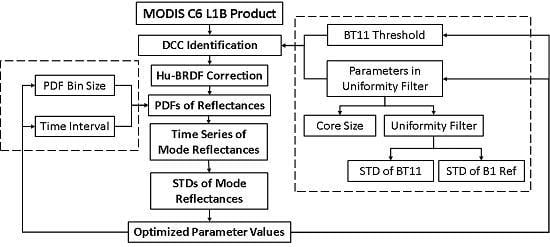
2.1. Background

The MODIS L1B product is generated by converting uncalibrated observations into calibrated observations using calibration parameters derived from the onboard calibrators, lunar and desert observations. A perfect invariant target calibration algorithm should reveal only the instrument degradation. If the calibration is accurate, the radiance over an invariant target should be stable within the specifications of the calibration uncertainty. However, no invariant target is perfect and would add noise on top of the instrument degradation. Therefore, an invariant target calibration algorithm can be evaluated by reducing the overall long-term standard error of the predicted fit. The purpose of our study is to assess the long-term stability of MODIS L1B product using an optimal DCCT. In order to downsize the large volume of daily global MODIS data (17+ years for Terra and 15+ years for Aqua), Doelling et al. [13] use the MODIS L1B data in the Tropical Western Pacific domain which has the greatest frequency of DCCs over the tropics. In this study, we utilize MODIS C6 aggregated L1B earth view data at 1 km resolution, Terra MOD021KM and Aqua MYD021KM (https://ladsweb.nascom.nasa.gov/), to assess the on-orbit calibration performance using the DCC technique. To obtain the greatest frequency of DCC samples from each granule and to reduce the data volume, MODIS L1B swath data with any pixel geo-located over the eastern Indian and western Pacific Oceans (30°S–30°N and 95°E–175°E) are used to identify the DCC samples for stability analyses. Since MODIS L1B algorithm incorporates a reflectance-based calibration, we use the reflectance data in MODIS L1B product instead of radiance data for DCC processing. Band 31 (10.78–11.28 μm) provides brightness temperature measurements required for the DCC pixel identification. The inter-comparison results of 11-µm brightness temperature (BT11) between MODIS and the Infrared Atmospheric Sounding Interferometer (IASI) found that the fluctuations of the biases between MODIS and IASI are less than 0.5 K for all band 31 detectors [22]. The stability of MODIS BT11 derives high-quality DCC identification. The MODIS L1B data covering the time period from July 2002 to October 2016 are used to assess the long-term calibration performance of MODIS RSB.

2.2. Identification of Deep Convective Clouds

The first step of DCC identification process is to use MODIS band 31 11-µm BT11 threshold value of 210 K to identify the potential DCCs [23]. The reflectance values from MODIS L1B data are computed over all the identified potential DCC samples. The DCC samples with reflectance impacted by saturation are flagged and excluded from further analyses. To avoid anisotropic conditions, the solar (SZA) and view zenith angles (VZA) are limited within 40° where DCCs are most isotropic [15,16]. The latitude is limited between (30°S–30°N) to identify DCCs in the tropical region. The potential DCCs identified by BT11 thresholds alone can be contaminated by optically thick ice clouds outside the core area of the DCC (e.g., [24,25,26]). In the second step, to avoid pixels that contain DCC cloud edges and anvils, a uniformity test is performed over a 3 by 3 pixel (1km spatial resolution) block surrounding the centered DCC pixel. The center DCC pixel is rejected if the BT11 standard deviation (STD) over the 3 by 3 pixel block is greater than 1 K or the RSB 1 (~0.65 µm) reflectance STD is greater than 3% of the average reflectance over the 3 by 3 block [15,16]. Figure 1 shows the MODIS pixel-level BT11 with SZA and VZA less than 40° by using all frames with valid BT11 values (Figure 1a,d), potential DCC frames with BT11 < 210 K before (Figure 1b,e) and actual DCC frames after (Figure 1c,f) the spatial uniformity test for one Terra L1B granule 2014305.0125. Confining SZA and VZA within 40° excludes the pixels impacted by anisotropic scattering. The criterion of BT11 < 210 K identifies a small portion of MODIS pixels as potential DCC pixels. The uniformity test decreases the frequency of DCC identified pixels. The histograms of BT11 over the DCC pixels change before (Figure 1e) and after (Figure 1f) the uniformity test accordingly. The uniformity test is necessary to choose the high-quality DCC pixels.

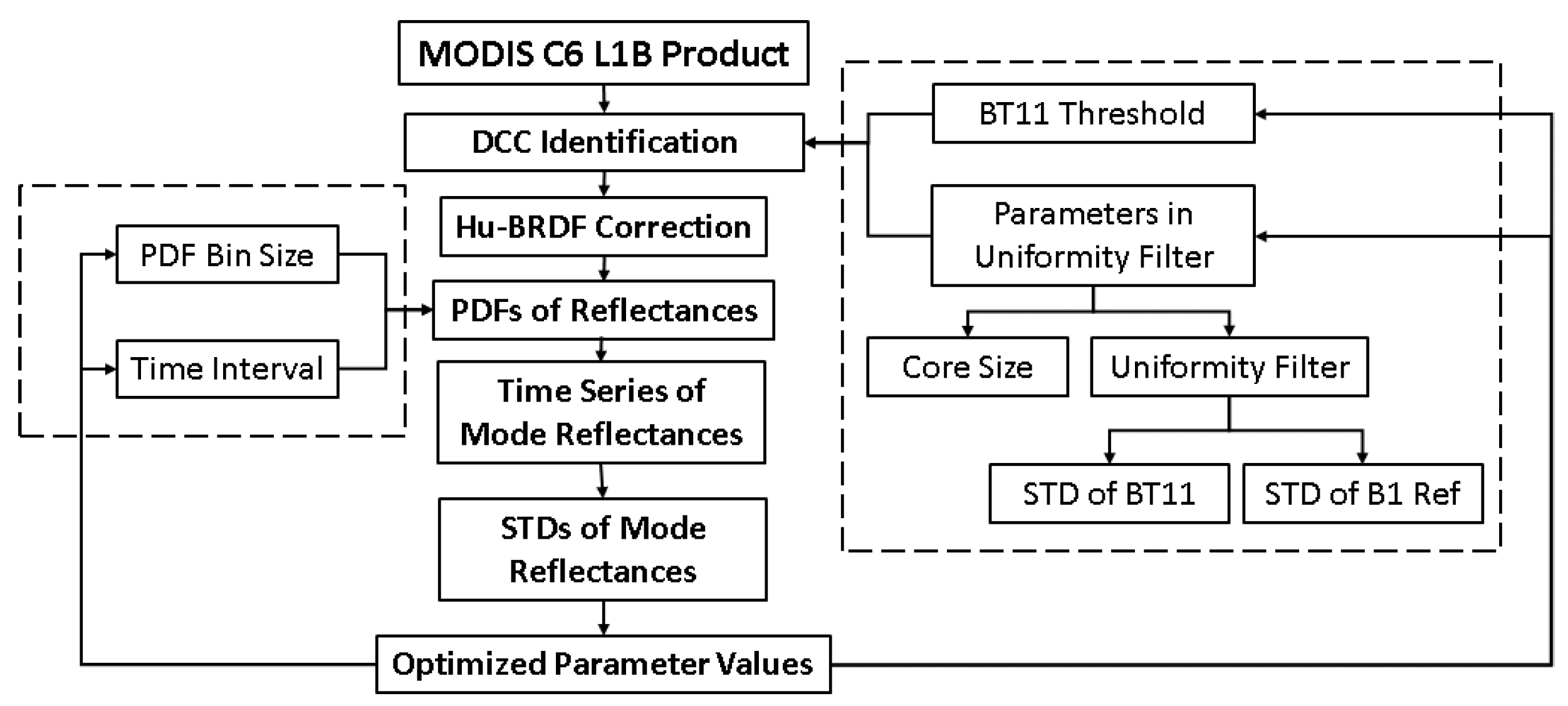
2.3. Derivation of Reflectance Trending Using the DCC Technique

In order to obtain a long-term trend and uncertainty for each band, all the identified DCC pixel reflectances during a given time interval are compiled into a PDF. Then the reflectance value corresponding to the peak probability density, i.e., mode reflectance, or the average reflectance over all the DCC samples is obtained from the PDF. The method of using mode reflectances from PDFs for DCC calibration is preferred over using average reflectances over all the DCCs for wavelengths less than 1 µm [15]. In order to simplify the operational DCCT method, only the mode reflectances are used to analyze the temporal STDs of the selected RSB. The success of this DCCT depends on identifying enough DCC samples that allow for a smooth and near-similar PDF over each data collection time interval. A monthly time interval is set as the data collection time in the baseline experiment. We compare the PDFs of the monthly reflectance and STDs of monthly mode reflectances for different RSB, with no BRDF corrections and with the BRDF corrections, as previously reported by Doelling et al. [13].

To investigate the potential impact of the BRDF effects on the reflectance at different wavelengths over the DCCs, we perform BRDF corrections to the reflectances using Hu et al.’s model [21] and compare the Hu-BRDF corrected results with the uncorrected results. The Hu et al. model [21] was designed for use with MODIS Visible and Infrared Scanner (VIRS) band 1 (0.65 µm). In order to avoid direct forward and backward scattering, the relative azimuth angle is restricted between 10 and 170 degrees [16]. Figure 2 shows the monthly PDFs of reflectance over DCCs with and without Hu-BRDF corrections in July for Terra and Aqua band 1 from July 2002 to October 2016, i.e., containing the July PDFs for 15 years. There are a substantial number, more than 100,000 per month [16], of DCC pixels, and the PDF curves are very smooth. Though the pixel frequency is low for some months, there are still around two million DCC pixels for Terra and around one million DCC pixels for Aqua each month. The PDFs with Hu-BRDF correction have less noise than the ones with no BRDF corrections for Terra and Aqua RSB 1, 3–4, and 18.

3. Sensitivity Tests

If no instrument uncertainty is involved, the PDF of DCC reflectance is a single-peak asymmetric density function with a long tail on the low reflectance side [15]. It is challenging to characterize the DCC reflectance PDF and DCC sample identification also depends on sensor measurements. The actual distribution of the measured DCC reflectance is the convolution of DCC asymmetric distribution and normal distribution of measurement uncertainty. Since the PDF is a statistical function of the measurement data, the uncertainty of the mode reflectance depends on the sample number and histogram processing parameters. The focus of our work is to minimize the uncertainty impact on the trending. Figure 3 indicates the diagram of the designed sensitivity test experiments showing the parameters to be optimized, and the Hu-BRDF correction for reflectance in DCCT.

In the baseline experiment, DCCT uses a BT11 threshold of 205 K for DCC identification, a uniformity filter of 1 K of BT11 STD and 3% of 0.65-µm reflectance STD over a spatial extent of 3 by 3 pixels for exclusion of DCC edges, a PDF bin reflectance interval of 0.001, and monthly time intervals or time steps. For all of the sensitivity tests, except for the tested parameter, all the other parameter values are as same as those in the baseline experiment, as shown in

Table 2. Parameter values in the baseline experiment and parameter value ranges in the sensitivity test experiments using the DCC technique (DCCT). BT: ~11-µm brightness temperature; Ref: 0.65-µm reflectance.

All Channels	BT11 Threshold (K)	Uniformity Filter Thresholds			PDF Bin (Ref)	Time Interval (Month)	BRDF
		BT11 (K)	Ref STD (%)	Extent (Pixel × Pixel)
Baseline DCCT	205	1	3	3 × 3	0.001	1	Hu
Sensitivity Tests	189–210	0.5–3	1, 3, 5	3 × 3, 5 × 5, 7 × 7, 9 × 9	0.0005–0.005	1, 3, 6, 12	Hu

. The optimal parameter values are chosen in their full parameter value spaces with ranges shown in Table 2 [13,15].

3.1. PDF Bin Interval

The success of DCCT relies on the fact that the DCC reflectances when analyzed collectively as a large ensemble are stable over time, with a small residual seasonal variation. An inadequately populated PDF may have distortion, and a fine bin size may cause a noisy curve or multiple peaks. The bin size impacts on the mode reflectances also depend on the magnitudes of the mode reflectances. If a noisy PDF has multiple mode peaks, the mode reflectance is calculated as the average over the multiple mode reflectance. A larger bin size may result in a smoother PDF but cause larger discretization steps between the monthly DCC reflectances. In the baseline test, we use a bin size of 0.001. In this subsection, we check the bin size effects on the uncertainties by using different bin size values from 0.0005 through 0.005.

No invariant target is perfect and would add noise on top of the instrument stability. The DCCT with the lowest STD to the regressed values is usually closest to detect the actual instrument performance. Small bin sizes may increase the standard error of the regression. The goal is to optimize the bin size to find the lowest standard error given the sampling frequency. Figure 4 shows the impacts of bin size on STDs of long-term mode reflectances for each RSB. The STDs are normalized to the fitted mode reflectance at the starting time point July 2002 in percentage. Figure 4 indicates that Hu-BRDF corrected results have lower STDs than the ones without BRDF correction for MODIS RSB 1, 3–4, and 18. For MODIS SWIR bands 5–7 and 26, Hu-BRDF correction is not recommended since it increases the STDs of the temporal mode reflectances. This is to be expected since the Hu model was intended for wavelengths near 0.65 µm [16,21].

To optimize the bin size in DCCT for MODIS calibration evaluation, we choose the bin size with the least temporal STD for each RSB. Overall, the bin size does not affect the uncertainties in reflectance significantly. For Terra and Aqua RSB 1, 3–6, and 18, all the bin size values can be used without deriving much difference in the STDs. Aqua has more noisy and inoperable detectors in the SWIR bands than Terra from prelaunch, which induces higher STDs in Aqua SWIR bands than in Terra SWIR bands. Overall, bin sizes of 0.035–0.005 are not recommended for Terra and Aqua band 7 (2.1 µm). However, the serious detector issue in Aqua RSB 6 does not affect the optimization of bin size because the variation and shape of STDs against bin size is similar to Terra RSB 6 (Figure 4). The optimal bin size is set as 0.002 for RSB 1, 3–5, 18 and 26 but set as 0.001 for RSB 6–7 due to the low magnitudes of their reflectances (see Section 3.4.1 for more details).

3.2. Data Collection Time Interval Effects

In this subsection, we check if the mode reflectances from PDFs over DCCs using different data collection time intervals affect the uncertainties in MODIS RSB. For different collection time intervals, the time periods of the data coverage are different. The data coverage time period is July 2002–October 2016 for monthly time interval, July 2002–September 2016 for three-monthly, July 2002–June 2016 for six-monthly, and January 2003–December 2015 for yearly time interval. The Terra and Aqua mode reflectance values are obtained from the reflectance PDFs over DCCs sampled over the certain collection time intervals of L1B data.

In Section 3.1, the bin sizes with the least trend STDs are used as a criterion to check for the optimal bin size. However, in each year, there are 12 data points for the monthly results, four data points for the three-monthly results, two data points for the six-monthly results, and one data point for the yearly results. The STDs of mode reflectances using different data collection time intervals are not comparable due to different numbers of data points. Figure 5 shows the STDs of DCC mode reflectances normalized to their corresponding first fitted values over different time intervals and STD changes relative to STD from baseline experiment in percentage for RSB 1, 3–7, 18, and 26. The results for bands 1, 3–4 and 18 are from the Hu-BRDF corrected reflectances, and from the non-BRDF corrected reflectances for the SWIR bands 5–7 and 26. There is an intrinsic seasonal cycle in the DCC reflectances due to the annually repeating movements of the DCCs mitigating with the sun and the satellite sampling angles. Since the DCC movement is nearly the same from year to year and the angles are replicated each year, the yearly results smooth out the DCC seasonal cycle and average out the short-term instrument noise. As expected, longer-time intervals decrease the STDs in Figure 5. All channels benefit from annual time intervals. The monthly time interval corresponds to the highest STD and the least STD is from using the yearly time interval for each RSB.

In the long-term stability monitoring and instrument lifetime trending assessment analyses of MODIS L1B product, the minimal time interval of three, or six, or 12 months for each RSB as shown in

Table 3. The minimum DCC sample collection time intervals in in the long-term stability monitoring for Terra and Aqua RSB 1, 3–7, 18, and 26 over July 2002–October 2016. The unit is in month.

	B1	B3	B4	B18	B5	B6	B7	B26
Terra	3	6	6	12	6	12	12	3
Aqua	3	6	12	12	12	12	6	12

is recommended to minimize the intrinsic seasonality and the uncertainty error in the DCCT results. However, in operational assessment using the DCCT, three, six or 12 months is too long to find any abnormal behavior in MODIS L1B calibration promptly. The seasonal cycle is small for RSB with wavelengths less than 1 µm and larger for RSB with longer wavelengths (Figure 5). If the user has a requirement for an uncertainty less than a certain value, Figure 5 can provide the smallest temporal interval to achieve the uncertainty required. For operational stability monitoring purposes, the monthly data collection time is recommended in the future standard MCST’s operational DCC technique.

3.3. Effects from Parameters in the Uniformity Test

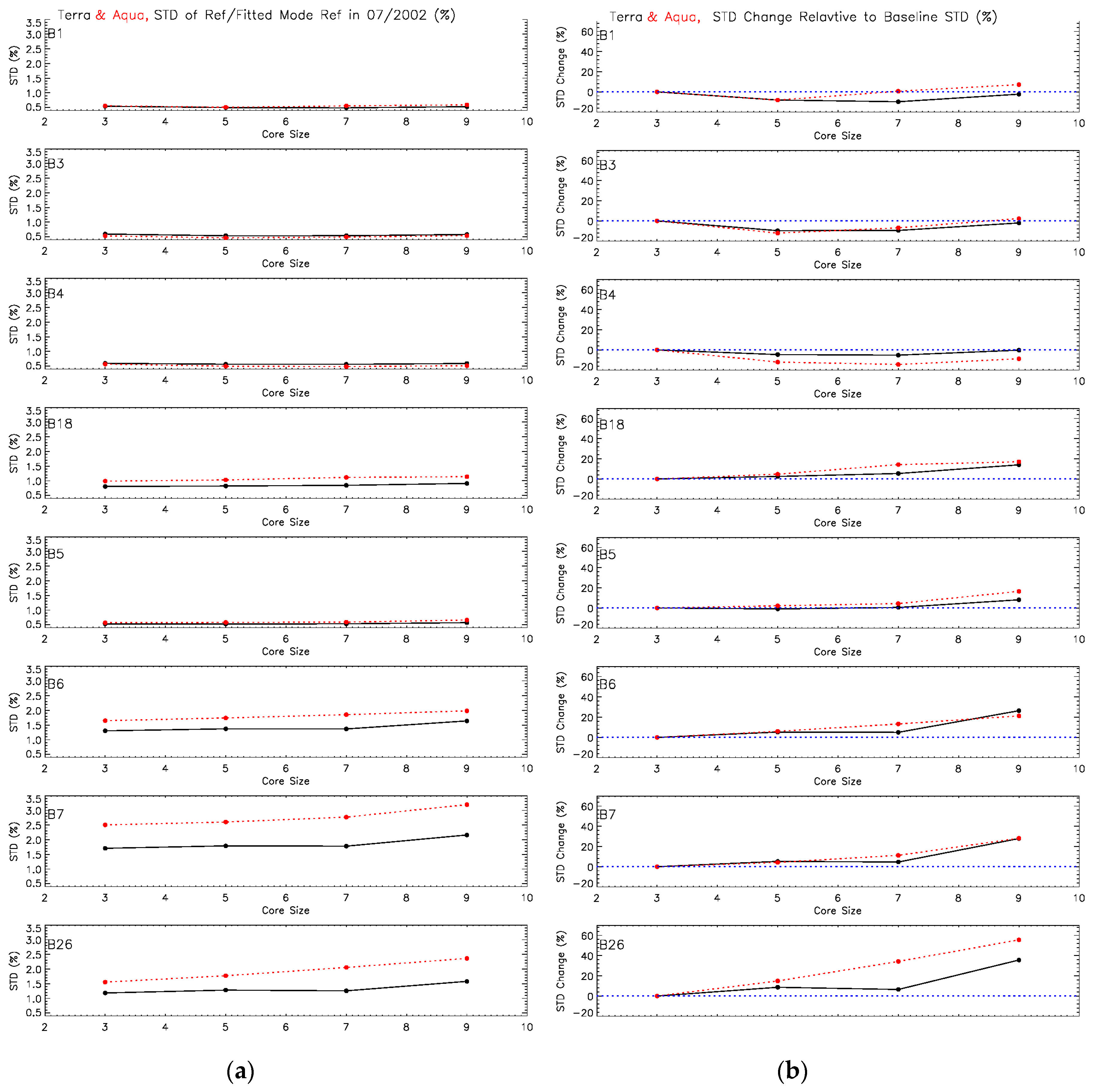
3.3.1. Core Size Extent Impact on the Uniformity Filter

We perform the uniformity test to avoid the DCC cloud edges and anvils as discussed in Section 2. In the baseline experiment using the DCC technique, surrounding each potential identified DCC pixel, a block of 8 neighboring pixels is chosen, i.e., with a core size of 3 by 3 pixels following Doelling et al. [15,16] and Wang and Cao [27]. Uniformity tests that incorporate larger core sizes would decrease the frequency of the identified DCC pixels by excluding anvils or DCC edges. Larger core sizes would be more likely to select DCC pixels located at the convective cloud cores, which should have greater reflectance uniformity [24,25,26] as shown in Figure 6. In this subsection, we use core sizes of 3 by 3, 5 by 5, 7 by 7, and 9 by 9 to evaluate the impact of the core size on the performance of the DCCT.

The identified DCC pixels located at the convective cloud cores using larger core sizes have higher reflectances than the DCC edges and anvils [24,25,26]. As predicted, the mode peaks of the reflectance PDFs shift towards right using larger core sizes as indicated in Figure 7. The average mode reflectance derived from a core size of 9 by 9 increases around 2.1% relative to that derived using a core size of 3 by 3. However, a larger core size reduces the number of DCC samples (Figure 7) and reduces the smoothness and the month-to-month similarity of the PDFs. With a core size of 9 by 9, insufficient monthly DCC samples generate noisy PDFs and unreliable mode peaks, hence high uncertainties in mode reflectances for some bands such as Terra RSB 4 and Aqua RSB 26. Figure 8a shows the STDs of monthly mode reflectances normalized to their corresponding fitted mode reflectances in July 2002 versus core size for Terra and Aqua RSB 1, 3–7, 18, and 26. Figure 8b shows the changes in STDs relative to those derived from the baseline experiment versus core size for Terra and Aqua RSB 1, 3–7, 18, and 26. The corresponding values are calculated using Hu-BRDF corrected reflectances over DCCs for RSB 1, 3–4 and 18, and non-BRDF corrected reflectance for RSB 5–7 and 26. Compromising the sufficient DCC samples for smooth PDFs, the uniformity of the DCCs, and the magnitude of STDs against core size, we recommend an optimal core size of 5 by 5 for RSB 1, 3–4 and 18, 3 by 3 for RSB 5–7 and 26 in the uniformity test.

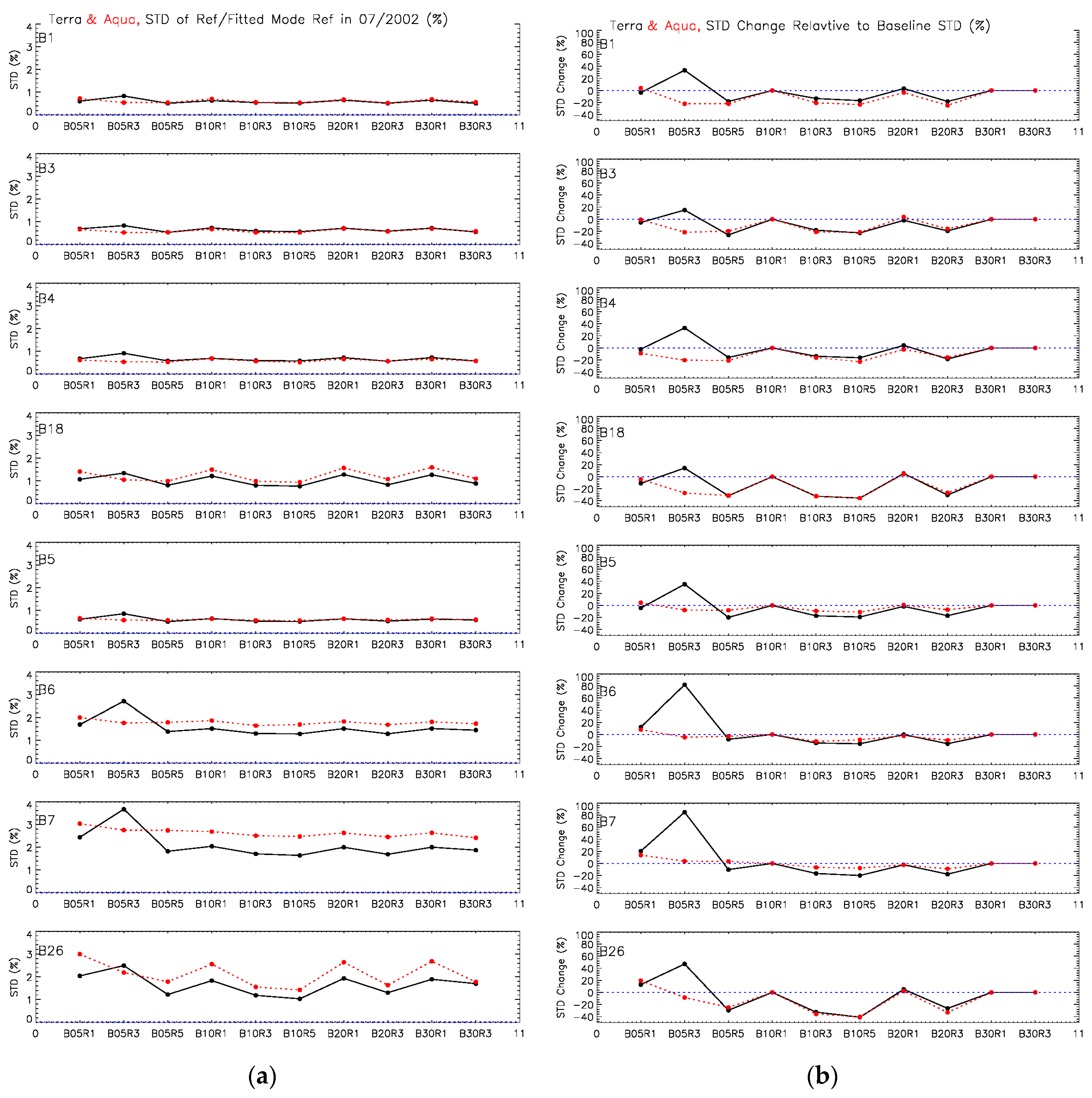
3.3.2. Criteria for Spatial Standard Deviations of Brightness Temperature and 0.65-µm Reflectance in the Uniformity Test

The homogeneity test identifies more uniform top or Lambertian part of the convection. In the baseline experiment, criteria of 1 K for BT11 STD and 3% for RSB 1 (~0.65 µm) reflectance STD over the 3 by 3 pixel block is used in the uniformity test [15,16]. In this subsection, we perform several sensitivity tests by varying the BT11 STD threshold by 0.5 K, 1 K, 2 K, or 3 K, and the RSB 1 reflectance STD threshold by 1%, 3%, or 5%. Higher thresholds exclude fewer heterogeneous DCCs after the uniformity test. In Figure 9, the x-axis label such as B05R1 means 0.5 K as the criteria for BT11 STD and 1% as the criteria for RSB 1 reference STD. In this study, we only perform the uniformity test experiments by combining any B05, B10 and B20 with R1, R3 and R5 except for B20R5, in addition with B30R1 and B30R3. These tests are enough to get the sensitivity of the DCCT to the two thresholds and to get the optimal threshold values with high uniformity. The variations in the STDs of the mode reflectances using different criteria combinations in Figure 9 indicate that RSB 26 is very sensitive to the criteria in the DCCT uniformity test. The optimal criteria are recommended as 1 K and 3%, or 1 K and 5% for BT11 STD and RSB 1 reflectance STD, respectively, for all the study Terra and Aqua RSB.

3.4. Brightness Temperature Threshold Effects

The DCC identification is dependent on the brightness temperature and the homogeneity of the visible reflectance and long-wave-infrared thermal temperature at the pixel level [16]. Previous studies [17,28,29,30] used BT11 thresholds between 190 K and 210 K to identify bright uniform DCC targets. Doelling et al. [13] carried out sensitivity tests to check the stability of the DCC technique in Aqua MODIS. A lower temperature threshold targets only DCC clouds rather than thick cirrus clouds, the latter of which are usually associated with the convective anvils [13]. A 2% (0.5%) increase in the mean (mode) reflectance was observed with each 5 K decrease in the BT11 threshold because a lower BT11 threshold removes the dark-pixel radiances in the PDF. However, a 94% reduction in DCC frequency and a noisy PDF was observed when reducing the threshold from 205 K to 195 K. The 190 K threshold produced a very noisy PDF owing to the lack of sufficient DCC samples. In this subsection, we systematically check the BT11 threshold effects on the Terra and Aqua MODIS DCC evaluation results and choose the optimal BT11 threshold values for different RSB.

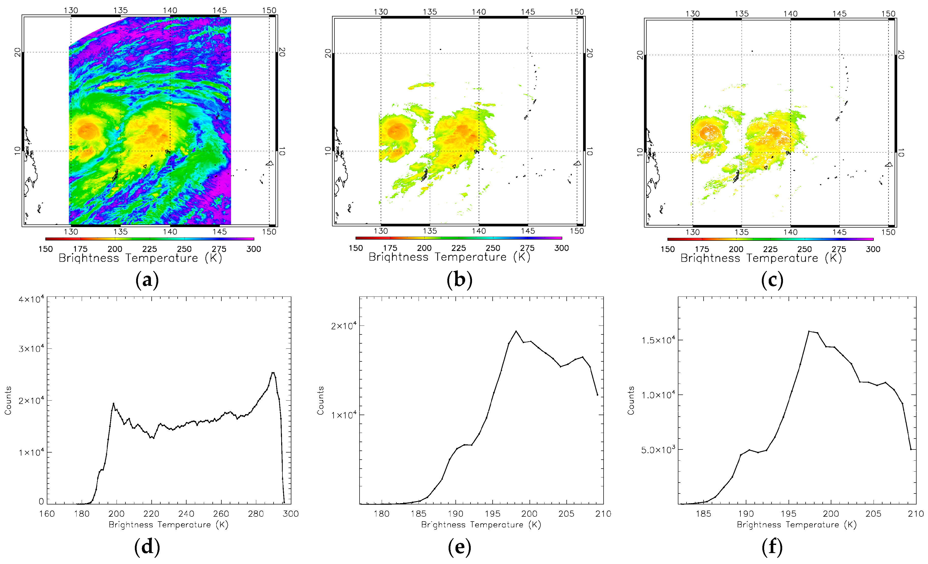
3.4.1. Monthly Frequency of DCC Pixels Reflectance versus BT11

The monthly DCC pixels are chosen using different BT11 thresholds from 189 K to 210 K for both Terra and Aqua MODIS. The monthly frequency of DCC samples is calculated during the study period from July 2002 to October 2016 with each BT11 threshold. Figure 10a shows the average monthly DCC number over the study time period versus BT11 threshold. Lower BT11 threshold decreases the average monthly frequency of DCCs significantly. Reducing the BT11 from 205 K to 195 K, the DCC sampling frequency was reduced by 85.3% for Terra RSB 1 and 84.4% for Aqua RSB 1 relative to the average monthly number at 205 K. The percentages of the reductions or increases in average monthly frequency of DCC samples relative to that from baseline versus different BT11 thresholds are shown in Figure 10b for Terra and Aqua RSB 1.

DCCs detected using lower BT11 thresholds are more likely to be associated with convective cores than those using greater BT11 thresholds [13,31]. DCC effective ice particle size decreases with cloud temperatures [31]. Generally, smaller particles in DCCs have higher reflectances [32,33]. The SWIR bands have great reduction of reflectance as the BT11 increases especially for SWIR band 26. In addition, RSB 26 is a cirrus cloud band and RSB 18 is water vapor band [34], both of which are strong water vapor absorption bands [32,34]. The convective cores of DCCs detected with a lower BT11 threshold reduce the water vapor absorptions by RSB 26 and 18. As a result, the largest percentage of change in average reflectance is with RSB 26, second largest with RSB 18, followed by RSB 1, 3–4, and the least with RSB 5–7 as shown in Figure 11a. Average reflectance is over all the DCCs which might include the misidentified DCCs. The DCCs corresponding to the mode peaks are less likely to be cirrus clouds. The results with mode reflectance are more reliable than those with average reflectance over all the identified DCCs. Figure 11b shows that the largest percentage of change in average mode reflectances is still with RSB 26, the second largest is with RSB 18 and 7, the third is with RSB 5–6, and the least is with 1 and 3–4. Overall, the impacts of ice particle size on the SWIR bands and the impacts of water vapor absorption on RSB 18 and 26 derive the greatest changes to the SWIR bands and RSB 18 in mode reflectances over DCCs.

3.4.2. Optimal Brightness Temperature Threshold

STDs of monthly mode reflectances using different BT11 thresholds are normalized to their corresponding first fitted mode reflectance in July 2002 (Figure 12a). The changes in STDs using different BT11 thresholds are calculated as percentage to the STDs derived from the baseline experiment with BT11 at 205 K for Terra and Aqua RSB 1, 3–7, 18, and 26 (Figure 12b). In principle, more DCC samples with a higher BT11 threshold in the DCC identification process should generate smoother PDFs and hence significantly reduce the STD of monthly mode reflectances for any RSB. However, increasing BT11 thresholds can misclassify the lower and warmer cirrus clouds as DCCs. DCCs are at the tropopause level that has minimal water vapor above it. Cirrus clouds are at the troposphere level which has more water vapor column above. The 1.38-µm RSB 26 and RSB 18 are strong water vapor absorption bands. Cores of DCCs identified by lower BT11 reduce the effects of water vapor absorption on RSB 26 and 18. In addition, the increase in ice particle size in DCCs by greater BT11 reduces the reflectance of RSB 26. As a result, STDs begin to increase with higher BT11 thresholds after BT11 reaches around 199 K for RSB 26 and 18 as shown in Figure 12.

Different MODIS RSB show different sensitivity to the BT11 threshold values in the DCC technique. RSB 6 and 7 have the largest magnitude in variations of STDs and trends (not shown) versus BT11, followed by RSB 5 and 26, and RSB 1, 3–4 and 18 have the least variations in STD variations. The underlying reasons for the different magnitudes in STD and trend variations for different RSB are explained as following.

(1)

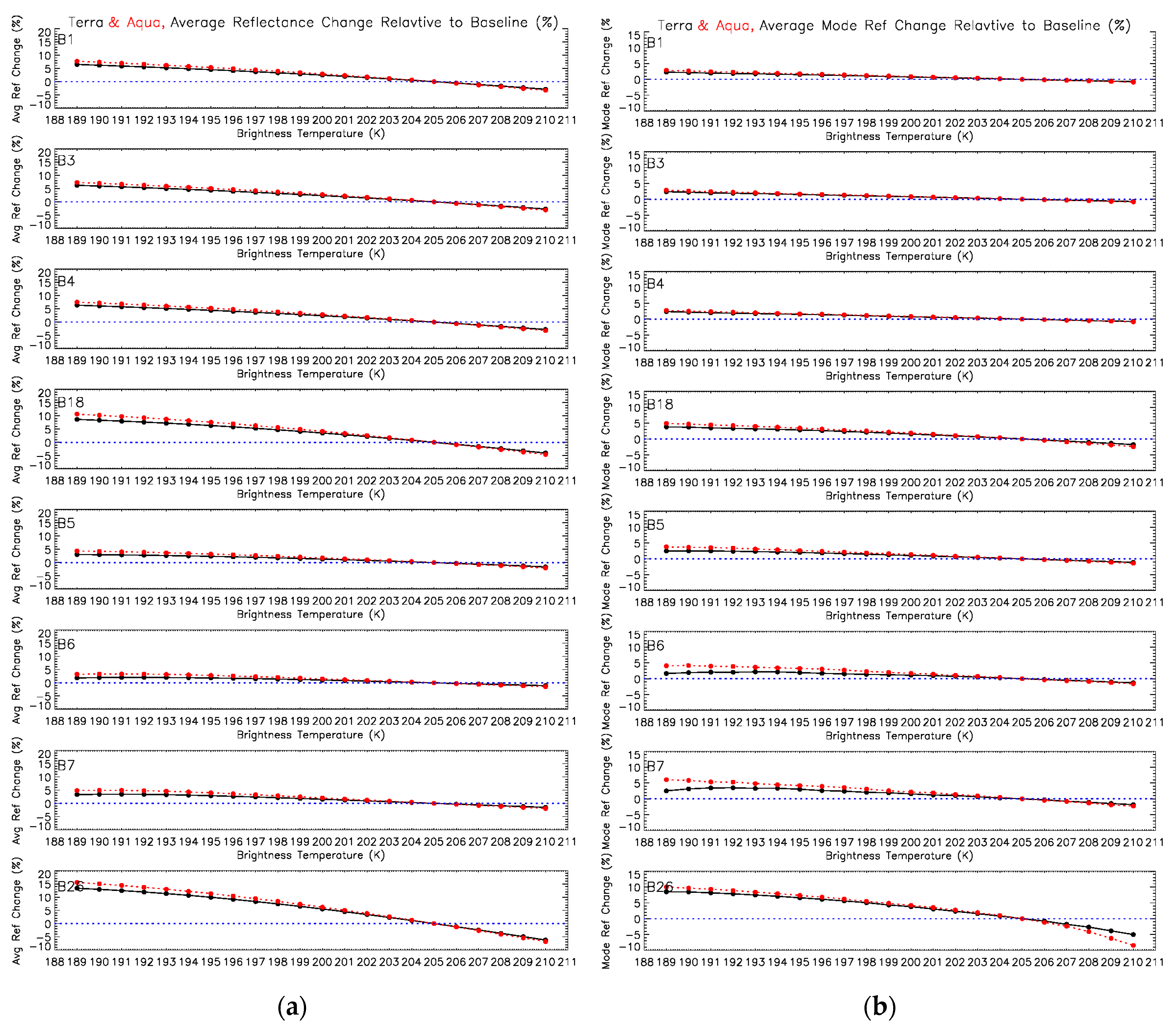
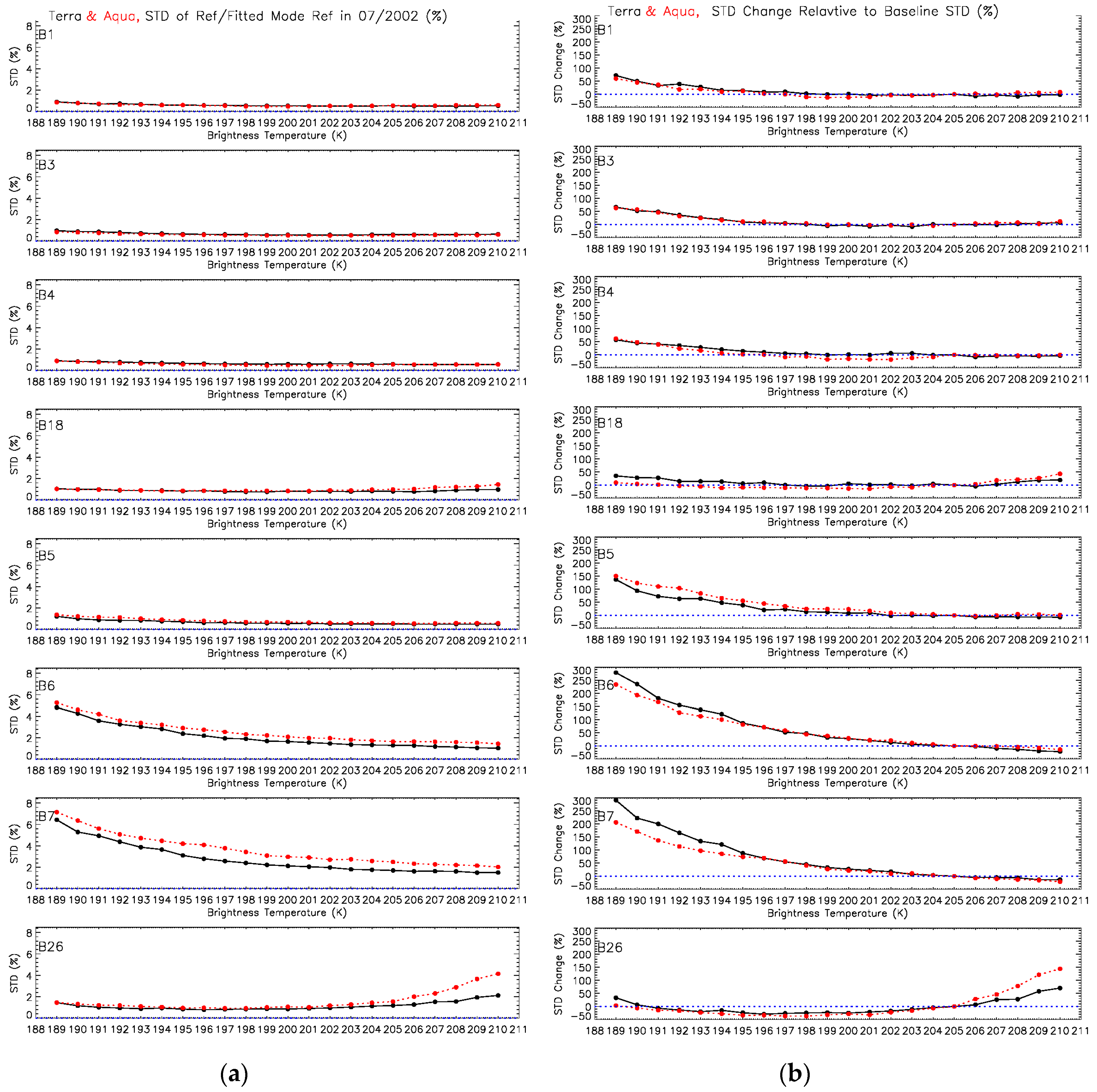
The magnitudes of monthly mode reflectances vary for different RSB. The mode reflectances are low for RSB 6–7, around 0.24 for RSB 6 and around 0.13 for RSB 7. The mode reflectances are at about the same level for RSB 5 and 26, around 0.67 for RSB 5 and around 0.6 for RSB 26. The highest mode reflectances are with RSB 1, 3–4 and 18, above 0.85. Therefore for the same absolute STD variation across all MODIS RSB, RSB 6–7 would have a larger relative STD change than the relative STD change for RSB 5 and 26, and RSB 1 and 3–4 would have the smallest relative STD change (Figure 12).

(2)

Reflectance is most sensitive to the particle size in clouds at wavelengths near 1.63 µm (RSB 6), 2.11 µm (RSB 7), then at wavelengths near 1.24 µm (RSB 5) and 1.38 µm (RSB 26) [32]. The ice particle size in the DCCs changes with brightness temperature [31]. The difference in reflectance responses to particle size derives great sensitivity of RSB to BT11 thresholds for the SWIR bands.

In this subsection, the magnitudes of STDs are used as a criterion to select the optimal BT11 threshold for DCC identification.

Table 4. The recommended ranges of brightness temperature threshold values (BT11) for Terra and Aqua MODIS RSB 1, 3–7, 18, and 26 (B1, B3–B7, B26).

	Terra BT11	Aqua BT11	Terra and Aqua BT11
B1	198–210	198–210	198–210
B3	195–210	195–210	195–210
B4	197–210	197–210	197–210
B18	197–206	189–206	197–206
B5	202–210	202–210	202–210
B6	203–210	203–210	203–210
B7	203–210	203–210	203–210
B26	190–206	189–205	190–205
All	203–206	203–205	203–205

lists the recommended BT11 threshold values for Terra and Aqua RSB. For RSB 1, 3–4 and 18 with wavelength less than 1 µm, a larger range of BT11 can be used as threshold for DCC identification. For the SWIR bands 5–7 and 26, especially for band 7, only a small range of BT11 is recommended. Column “Terra and Aqua BT11” in Table 4 lists the BT11 thresholds that work as optimal BT11 both for each Terra and Aqua RSB. It shows that any BT11 threshold between 203 K and 205 K for all Terra and Aqua RSB is recommended to identify the DCC pixels.

3.5. Optimized DCCT Parameters

As derived from the sensitivity experiments, the optimal parameter values utilized in the standard operational MCST DCCT calibrations are shown in the following

Table 5. Optimal parameter values as recommended for all the RSB.

Baseline DCCT	BT Threshold (K)	Uniformity Filter Thresholds			PDF Bin (Ref)	Time Interval	BRDF
		BT11 (K)	Ref (%)	Extent (Pixel × Pixel)
B1	205	1	3, 5	5 × 5	0.002	monthly	Hu
B3	205	1	3, 5	5 × 5	0.002	monthly	Hu
B4	205	1	3, 5	5 × 5	0.002	monthly	Hu
B18	205	1	3, 5	5 × 5	0.002	Monthly	Hu
B5	205	1	3, 5	3 × 3	0.002	Monthly	none
B6	205	1	3, 5	3 × 3	0.001	monthly	none
B7	205	1	3, 5	3 × 3	0.001	monthly	none
B26	205	1	3, 5	3 × 3	0.002	monthly	none

. For the long-term stability test of MODIS L1B product, six-monthly or yearly data collection time interval is recommended to minimize the seasonality of MODIS L1B product. These optimal parameter values in MODIS DCCT are wavelength dependent. The optimal MODIS DCCT parameter values can also be recommended for the Visible Infrared Imaging Radiometer Suite (VIIRS) instruments onboard the joint NASA/NOAA Suomi National Polar-orbiting Partnership (SNPP) and the future operational Joint Polar Satellite System (JPSS) satellites.

4. Comparisons between the Uncertainty Errors Using the Optimized DCC Technique, Desert and Dome-C Observations

MCST uses Libya-4 and Dome-C observations to operationally evaluate the stability of the MODIS L1B product. Here the trend uncertainties from the optimized DCC technique for each RSB is compared with that derived from Libya-4 and Dome-C data. Libya-4 data are collected every 16 days, which are significantly contaminated by the atmospheric absorption for some of the SWIR bands [10,14]. Dome-C is located in Antarctica. It provides very stable conditions of surface properties such as albedo, emissivity, plus an extremely dry and clear atmosphere. The disadvantages are a relatively short period (~4 months) of available data for RSB collected at high solar zenith angles. Due to the favorable atmospheric conditions, Dome-C is widely used as a ground calibration reference site for satellite sensors. However, Dome-C is viewed under oblique sun conditions and the signal to noise ratio (SNR) is small [10,14]. RSB 5–7 with weak reflectance are not monitored using Dome-C data. RSB 26 and 18 are not monitored using Libya-4 or Dome-C data due to the strong water vapor absorption effects. Stability is not monitored at Libya-4 for Aqua RSB 6 due to the noisy or dead detector issues.

Table 6. Terra (T) and Aqua (A) standard deviations of the monthly reflectances from DCCT, Libya-4 and Dome-C in percentage for (DCCT) baseline, optimized DCC (O-DCCT), Libya-4 and Dome-C over July 2002–October 2016 for all the RSB. The optimized parameters in DCCT are listed in Table 5. The unit is percentage of STDs to their corresponding fitted reflectance values in July 2002.

Terra				Band	Aqua
DCCT	O-DCCT	Libya-4	Dome-C		DCCT	O-DCCT	Libya-4	Dome-C
0.54	0.50	1.15	2.59	B1	0.56	0.49	1.00	2.15
0.59	0.51	1.51	1.70	B3	0.53	0.45	1.74	1.22
0.59	0.59	1.15	2.72	B4	0.57	0.47	1.33	2.34
0.72	0.67			B18	0.77	0.78
0.52	0.51	0.92		B5	0.58	0.54	0.87
1.37	1.30	1.00		B6	1.74	1.64
1.79	1.70	2.33		B7	2.60	2.50	1.85
1.28	1.18			B26	1.77	1.50

compares the uncertainties between the baseline and optimized DCC, Libya-4, and Dome-C. Results from DCCT have the lowest uncertainties for RSB with wavelengths less than 1 µm. The DCC uncertainties are greater for the SWIR bands. However, DCCT can be applied across all MODIS RSB that do not saturate. For RSB 7, the Libya-4 and DCC uncertainties are mixed between Terra and Aqua. In addition, the optimized channel DCCT has reduced the trend uncertainty when compared with the baseline DCCT for most channels. DCCT is an important MODIS operational stability monitoring tool to ensure the highest quality MODIS data for users.

5. Conclusions

Both MODIS instruments have been operating beyond their designed lifetime. To evaluate the performance of the on-orbit calibration algorithms, the stability of Terra and Aqua MODIS Level 1B product is monitored using the DCC technique for RSB 1, 3–7, 18, and 26 over the study time period from July 2002 to October 2016.

We carry out several sensitivity experiments to optimize the key parameters in the DCC technique such as the BT11 threshold for DCC identification, criteria and core size in the uniformity test to exclude the DCC edges, bin size in the histogram process to get the mode reflectance values, and the time interval of the DCC sampling. The goal is to optimize the parameters with the lowest standard error. The optimal parameter values listed in Table 5 will be incorporated in the MCST operational DCC technique for future evaluations of MODIS on-orbit calibration performance.

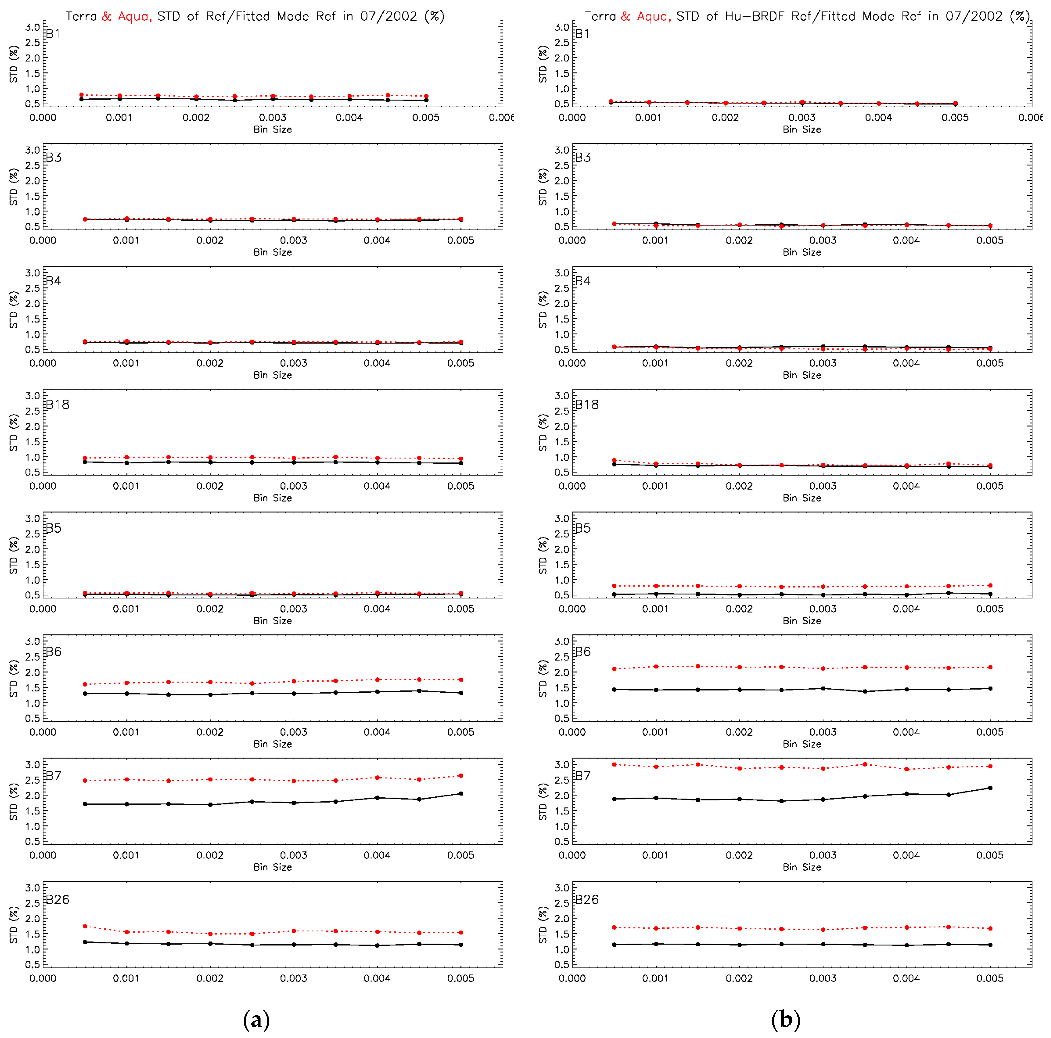
1

The bin size in the histogram processing has minimal impact on the stability of the DCC technique. The largest impact is on the SWIR bands 6–7, and the difference in the STDs compared to those from the baseline is less than 20%. Based on the magnitude of the STDs and the stability of the trends against bin size, the optimal bin size value is set as 0.002 for RSB 1, 3–5, 18, and 26, and 0.001 for RSB 6–7.

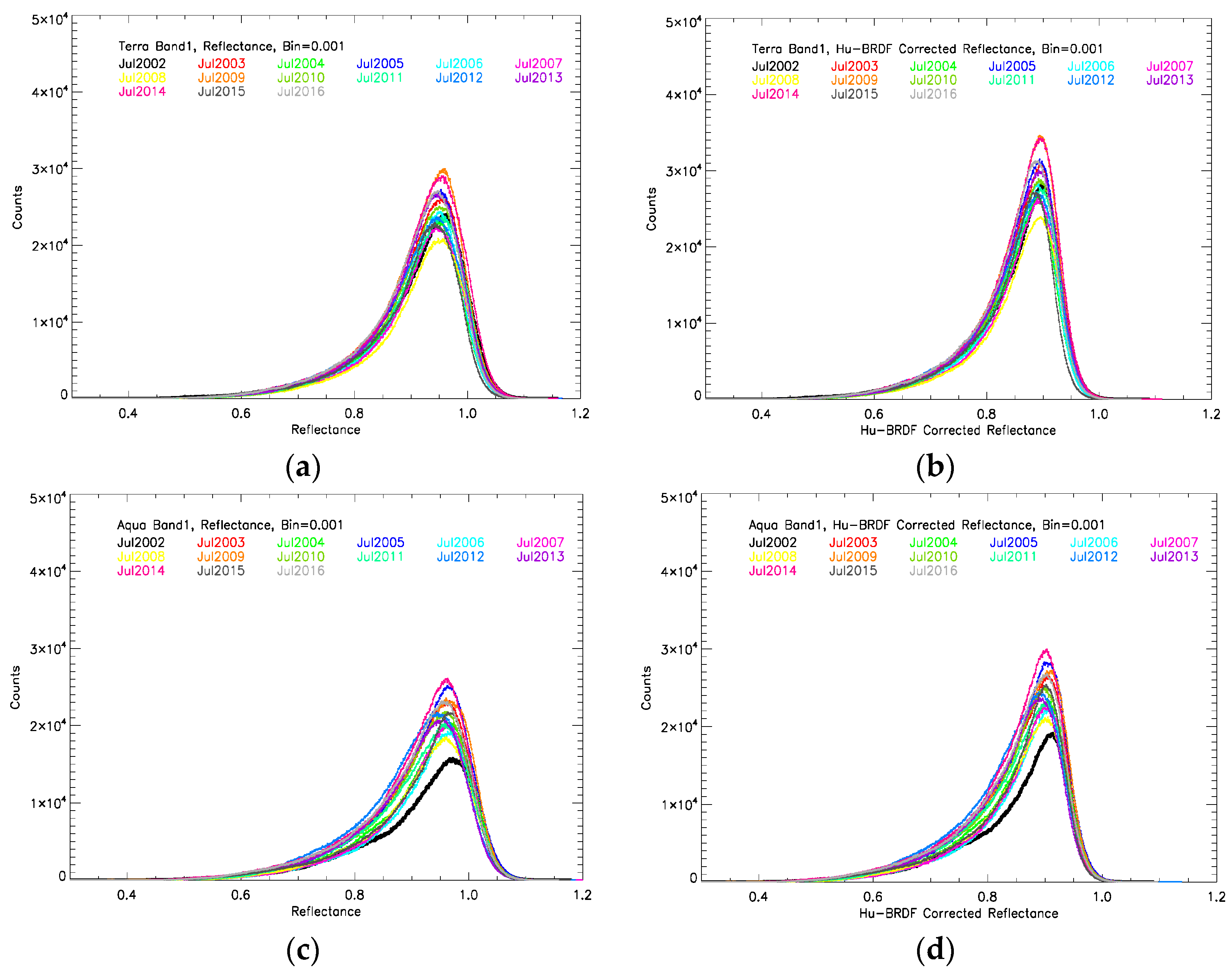
2

The BRDF correction model designed by Hu et al. (2004) for the VIRS at wavelength of 0.65 µm is applied to the results using the baseline method for all channels. For wavelengths less than 1 µm, the Hu model reduces the trend uncertainty. However, for the SWIR channels, the Hu model is inadequate and may increase the trend standard error.

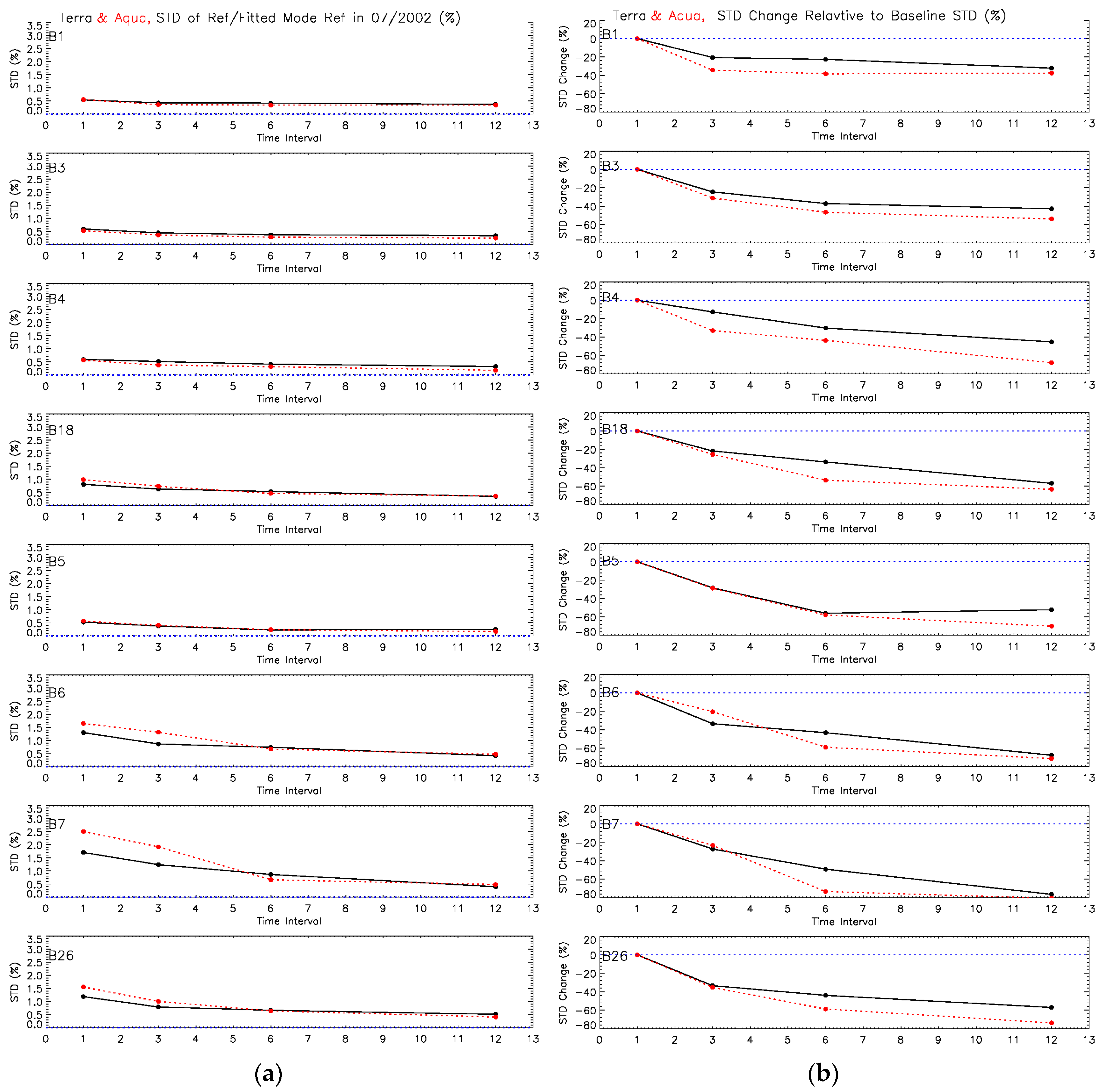
3

Increasing the time interval from one month to a year can reduce the intrinsic seasonality and the uncertainty error in the DCCT results. The seasonal cycle is small for RSB with wavelengths less than 1 µm and larger for RSB with longer wavelengths. The seasonal cycle of DCC properties mostly affects the SWIR bands that are impacted by cloud microphyiscs. For long-term evaluation of the performance of MODIS calibrations, the minimal time interval of 3, or 6, or 12 months are recommended. However, for operational stability monitoring purposes, monthly time interval is recommended as the optimal data collection time in the future standard MCST operational DCC technique. If the user has a requirement for an uncertainty less than a certain value, Figure 5 can provide the smallest temporal interval to achieve the uncertainty required.

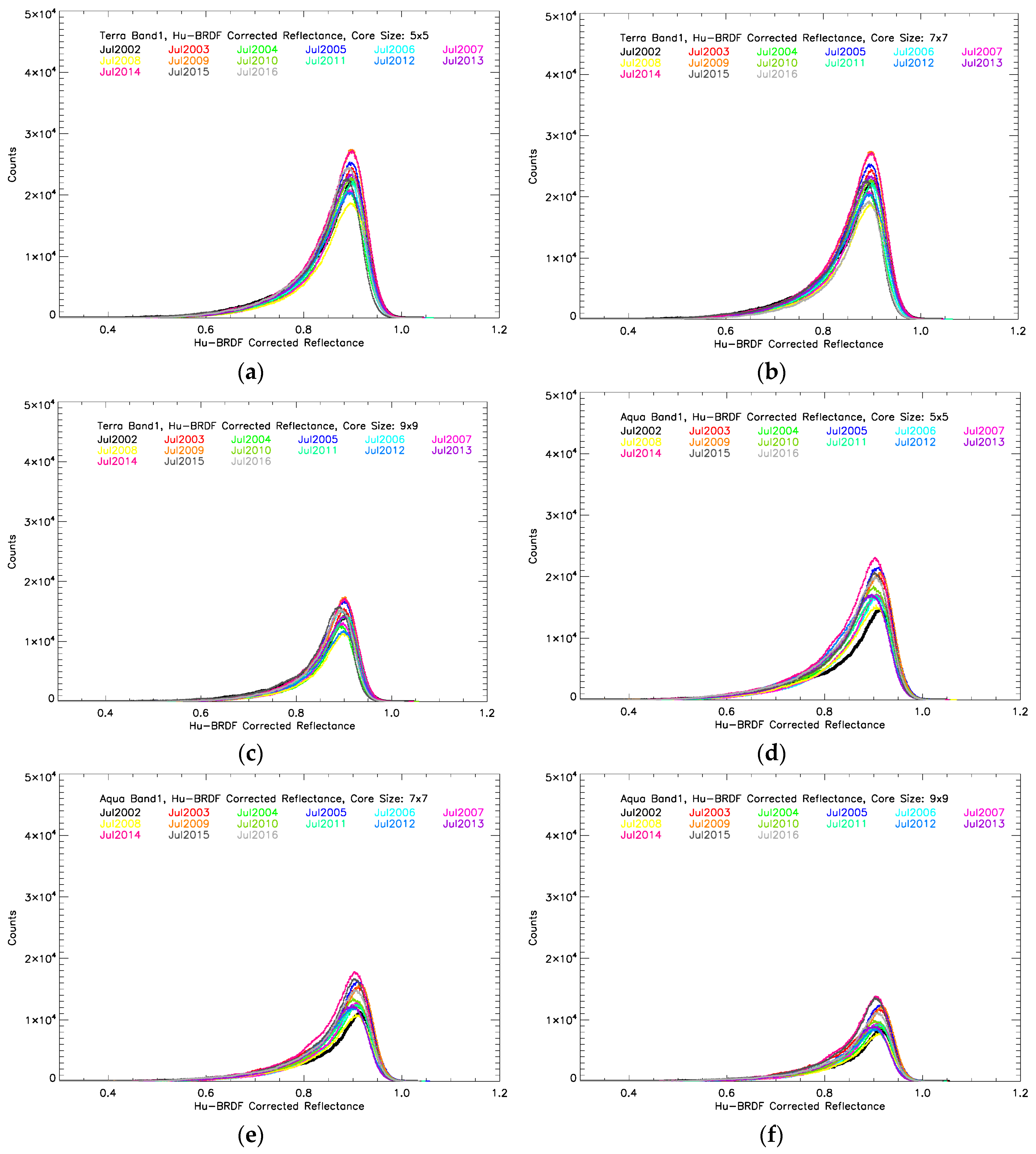
4

The uniformity test parameters of the BT11 STD, the RSB 1 reflectance STD and the spatial extent used to compute the STD play an important role in the DCCT to exclude the heterogeneous DCC samples. The criteria of BT11 STD and RSB 1 reflectance STD as 1 K and 3%, or 1 K and 5%, respectively, are recommended as optimal uniformity filter thresholds for the MODIS performance monitoring using DCCT. Using larger core sizes results in actual DCCs with higher uniformity, but shrinks the number of the DCC samples and reduces the smoothness of the PDFs. By balancing the core size with sampling frequency, a core size of 5 by 5 for RSB 1, 3–4 and 18 and 3 by 3 for RSB 5–7 and 26 is recommended in the uniformity test.

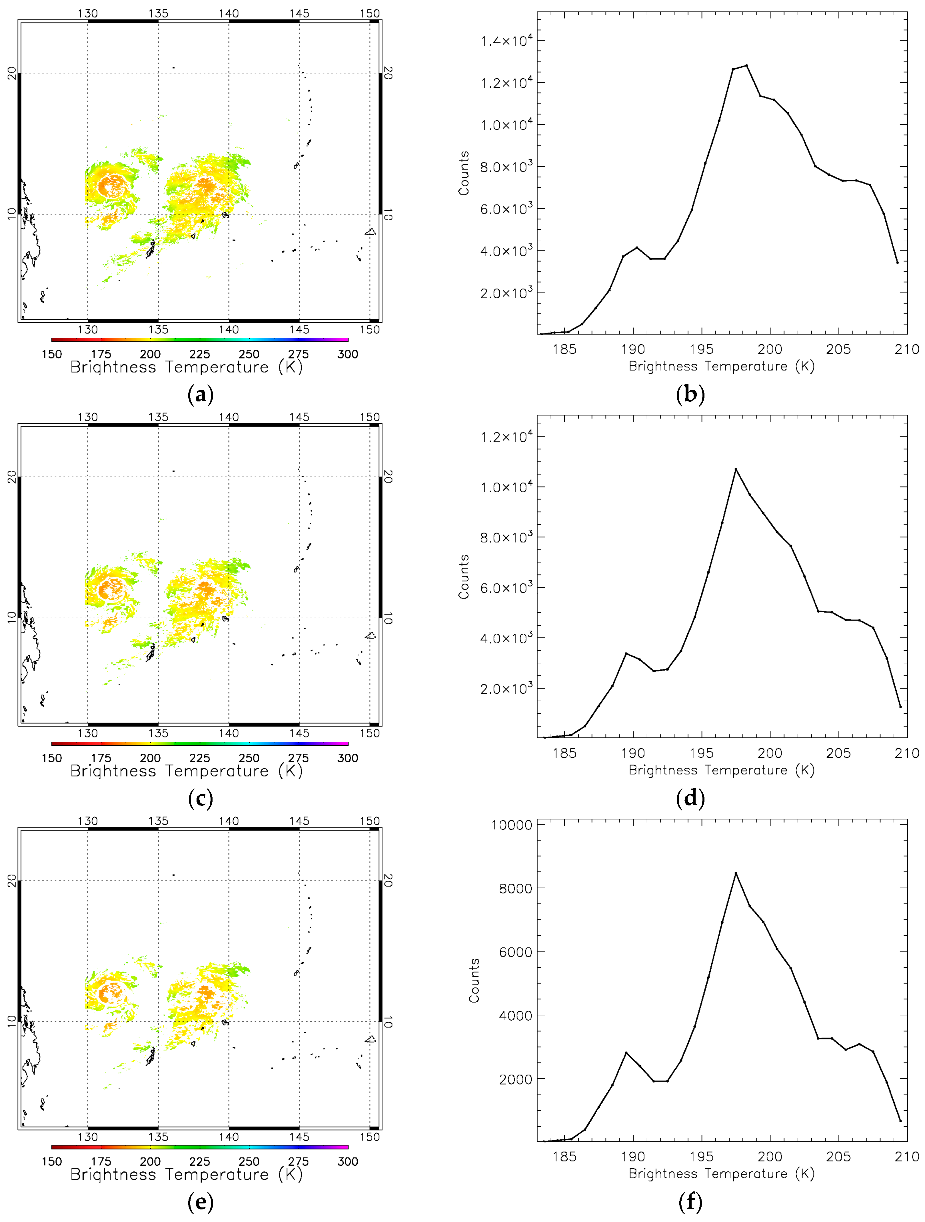
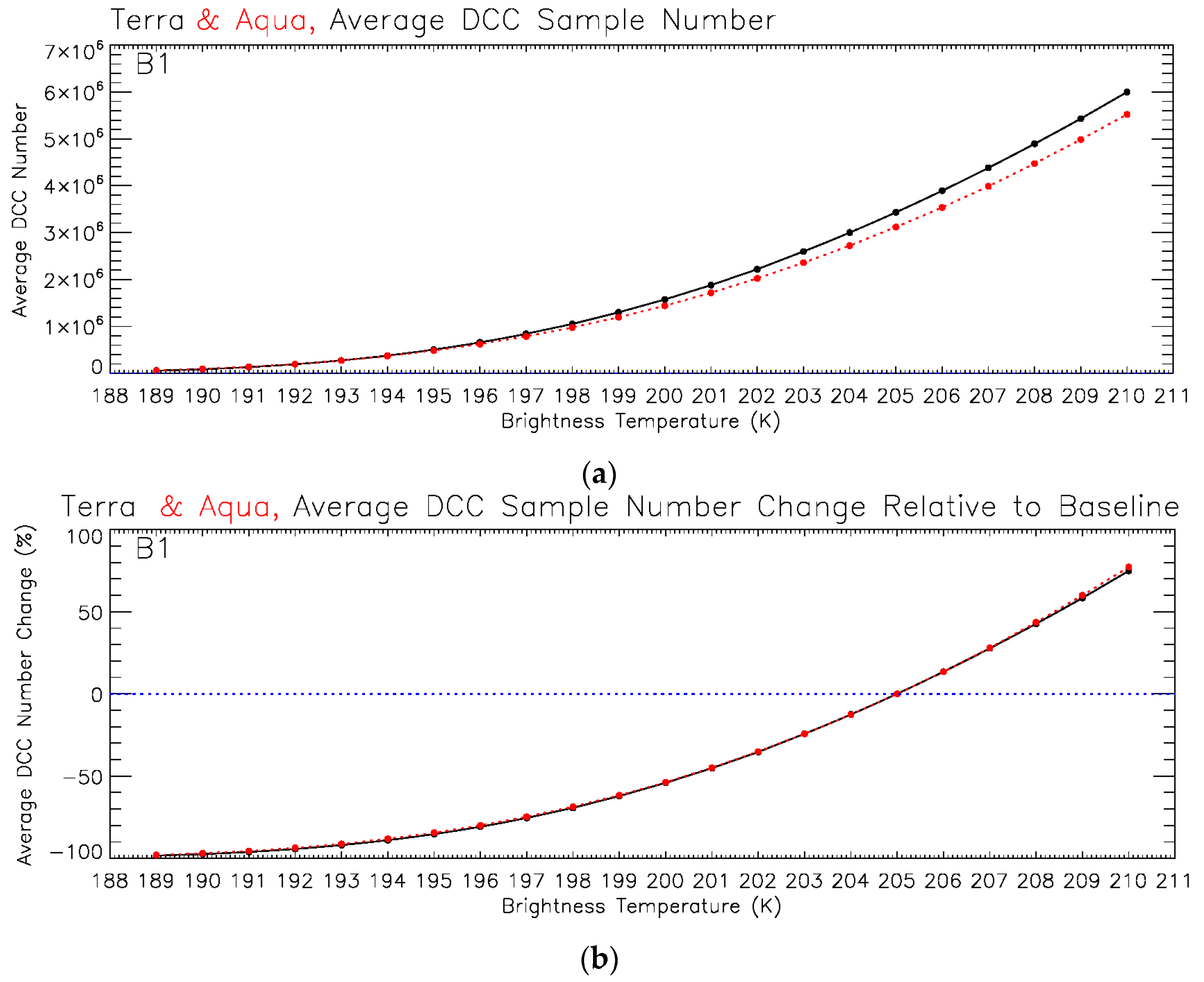
5

The DCC technique is most sensitive to the BT11 threshold in the DCC identification. Increasing the BT11 thresholds can increase the DCC sampling, leading to more predictable PDF shapes and therefore more stable mode reflectances. However, DCCs identified using lower BT11 thresholds are more likely to be associated with convective cores than those using greater BT11 thresholds. As a result, the trend uncertainties will decrease with increasing BT11 and remain constant between 205 K and 210 K. This does not hold true for band 26 and 18, for which the trend uncertainty starts increasing rapidly when BT11 is greater than 205 K. With increasing BT11 thresholds, lower and warmer cirrus clouds are misidentified as DCCs. The water vapor column above them strongly affects the reflectance of RSB 26 and 18, and hence induces larger uncertainties [32,34]. BT11 threshold is recommended between 203 and 205 K for all of the studied Terra and Aqua RSB.

Using the optimal parameter values, we compare the uncertainties derived from the baseline DCC experiment, the optimized DCC experiment, the Libya-4, and Dome-C. Because DCC observations are minimally impacted by atmospheric water vapor absorption, the standard error of regression for the DCC mode reflectance decreases significantly when compared to those from the Libya-4 and Dome-C invariant ground sites except for the SWIR bands at the Libya-4 site (Table 6). The optimal parameter values in MODIS DCCT are wavelength dependent. VIIRS is one of the key earth-observing instruments onboard SNPP and future JPSS. DCCs as invariant earth targets can be utilized to facilitate the calibration transfer from MODIS to VIIRs and other instrument by the Global Space-based Inter-Calibration System (GSICS) operational community [35]. The DCCT have been applied to the stability assessment of VIIRS RSB (M-bands, M1–M5, M7–M11, and I-bands, I1–I3) except for band M6 [27,28,36]. The parameter optimization of DCCT can be referenced in the VIIRS stability monitoring and to improve the assessment accuracy.

References

- Xiong, X.; Sun, J.; Barnes, W.; Salomonson, V.; Esposito, J.; Erives, H.; Guenther, B. Multi-year On-orbit Calibration and Performance of Terra MODIS Reflective Solar Bands. IEEE Trans. Geosci. Remote Sens. 2007, 45, 879–889. [Google Scholar] [CrossRef]
- Xiong, X.; Wenny, B.; Barnes, W. Overview of NASA Earth Observing Systems Terra and Aqua Moderate Resolution Imaging Spectroradiometer Instrument Calibration Algorithms and On-orbit Performance. J. Appl. Remote Sens. 2009, 3, 032501. [Google Scholar] [CrossRef]
- Xiong, X.; Sun, J.; Xie, X.; Barnes, W.; Salomonson, V. On-Orbit Calibration and Performance of Aqua MODIS Reflective Solar Bands. IEEE Trans. Geosci. Remote Sens. 2010, 48, 535–546. [Google Scholar] [CrossRef]
- Sun, J.; Xiong, X.; Barnes, W.; Guenther, B. MODIS Reflective Solar Bands On-Orbit Lunar Calibration. IEEE Trans. Geosci. Remote Sens. 2007, 45, 2383–2393. [Google Scholar] [CrossRef]
- Sun, J.; Xiong, X. Solar and lunar observation planning for Earth-observing sensor. SPIE Remote Sens. 2011. [Google Scholar] [CrossRef]
- Sun, J.; Xiong, X.; Angal, A.; Chen, H.; Wu, A.; Geng, X. Time-Dependent Response Versus Scan Angle for MODIS Reflective Solar Bands. IEEE Trans. Geosci. Remote Sens. 2014, 52, 3159–3174. [Google Scholar] [CrossRef]
- Xiong, X.; Cao, C.; Chander, G. An Overview of Sensor Calibration Inter-comparison and Applications. Front. Earth Sci. China 2010, 4, 237–252. [Google Scholar] [CrossRef]
- Xiong, X.; Wu, A.; Wenny, B.; Choi, J.; Angal, A. Progress and Lessons from MODIS Calibration Inter-comparison Using Ground Test Sites. Can. J. Remote Sens. 2010, 36, 540–552. [Google Scholar] [CrossRef]
- Wu, A.; Xiong, X.; Cao, C. Examination of Calibration Performance of Multiple POS Sensors Using Measurements over the Dome C Site in Antarctica, Sensors, Systems, and Next Generation Satellites XII. SPIE Remote Sens. 2008. [Google Scholar] [CrossRef]
- Wu, A.; Xiong, X.; Doelling, D.R.; Morstad, D.; Angal, A.; Bhatt, R. Characterization of Terra and Aqua MODIS VIS, NIR, and SWIR Spectral Bands’ Calibration Stability. IEEE Trans. Geosci. Remote Sens. 2013, 51, 4330–4338. [Google Scholar] [CrossRef]
- Kwiatkowska, E.J.; Franz, B.A.; Meister, G.; McClain, C.R.; Xiong, X. Crosscalibration of Ocean-Color Bands from Moderate-Resolution Imaging Spectrometer on Terra Platform. Appl. Opt. 2008, 47, 6796–6810. [Google Scholar] [CrossRef] [PubMed]
- Meister, G.; McClain, C.R. Point-spread function of the ocean color bands of the Moderate Resolution Imaging Spectroradiometer on Aqua. Appl. Opt. 2010, 49, 6276–6285. [Google Scholar] [CrossRef] [PubMed]
- Doelling, D.R.; Morstad, D.; Scarino, B.R.; Bhatt, R.; Gopalan, A. The characterization of deep convective clouds as an invariant calibration target and as a visible calibration technique. IEEE Trans. Geosci. Remote Sens. 2013, 51, 1147–1159. [Google Scholar] [CrossRef]
- Doelling, D.R.; Wu, A.; Xiong, X.; Scarino, B.R.; Bhatt, R.; Haney, C.O.; Morstad, D.; Gopalan, A. The radiometric stability and scaling of collection 6 Terra- and Aqua-MODIS VIS, NIR, and SWIR spectral bands. IEEE Trans. Geosci. Rem. Sens. 2015, 53, 4520–4535. [Google Scholar] [CrossRef]
- Doelling, D.R.; Nguyen, L.; Minnis, P. On the use of deep convective clouds to calibrate AVHRR data. In Proceedings of the Optical Science and Technology, the SPIE 49th Annual Meeting, International Society for Optics and Photonics, Denver, CO, USA, 2–6 August 2004. [Google Scholar]
- Doelling, D.R.; Morstad, D.L.; Bhatt, R.; Scarino, B. Algorithm Theoretical Basis Document (ATBD) for Deep Convective Cloud (DCC) Technique of Calibrating GEO Sensors with Aqua-MODIS for GSICS, GSICS. Available online: http://gsics.atmos.umd.edu/pub/Development/AtbdCentral/GSICS_ATBD_DCC_NASA_2011_09.pdf (accessed on 27 May 2017).
- Aumann, H.H.; Pagano, T.; Hofstadter, M. Observations of deep convective clouds as stable reflected light standard for climate research: AIRS evaluation. SPIE 2007. [Google Scholar] [CrossRef]
- Fougnie, B.; Bach, R. Monitoring of radiometric sensitivity changes of space sensors using deep convective clouds: Operational application to PARASOL. IEEE Trans. Geosci. Remote Sens. 2009, 47, 851–861. [Google Scholar] [CrossRef]
- Chang, T.; Xiong, X.; Angal, A.; Mu, Q. Assessment of MODIS RSB detector uniformity using deep convective clouds. J. Geophys. Res. Atmos. 2016, 121, 4783–4796. [Google Scholar] [CrossRef]
- Mu, Q.; Wu, A.; Chang, T.; Angal, A.; Link, D.; Xiong, X.; Doelling, D.R.; Bhatt, R. Assessment of MODIS on-orbit calibration using a deep convective cloud technique. In Proceedings of the SPIE 9972, Earth Observing Systems XXI, San Diego, CA, USA, 28 August–1 September 2016. [Google Scholar]
- Bhatt, R.; Doelling, D.R.; Angal, A.; Xiong, X.; Scarino, B.; Gopalan, A.; Haney, C.O.; Wu, A. Characterizing response versus scan-angle for modis reflective solar bands using deep convective clouds. J. Appl. Remote Sens. 2016, 11, 016014. [Google Scholar] [CrossRef]
- Li, Y.; Wu, A.; Xiong, X. Evaluating Calibration of MODIS Thermal Emissive Bands Using Infrared Atmospheric Sounding Interferometer Measurements. Proc. SPIE 2013, 8724. [Google Scholar] [CrossRef]
- Hu, Y.B.; Wielicki, B.A.; Yang, P.; Stackhouse, P.W., Jr.; Lin, B.; Young, D.F. Application of deep convective cloud albedo observation to satellite-based study of the terrestrial atmosphere: Monitoring the stability of spaceborne measurements and assessing absorption anomaly. IEEE Trans. Geosci. Remote Sens. 2004, 42, 2594–2599. [Google Scholar]
- Tian, B.; Soden, B.J.; Wu, X. Diurnal cycle of convection, clouds, and water vapor in the tropical upper troposphere: Satellites versus a general circulation model. J. Geophys. Res. 2004, 109, D10101. [Google Scholar] [CrossRef]
- Hong, G.; Heygster, G.; Miao, J.; Kunzi, K. Detection of tropical deep convective clouds from AMSU-B water vapor channels measurements. J. Geophys. Res. 2005, 110, D05205. [Google Scholar] [CrossRef]
- Liu, C.; Zipser, E.J.; Nesbitt, S.W. Global distribution of tropical deep convection: Different perspectives from TRMM infrared and radar data. J. Clim. 2007, 20, 489–503. [Google Scholar] [CrossRef]
- Wang, W.; Cao, C. DCC radiometric sensitivity to spatial resolution, cluster size, and LWIR calibration bias based on VIIRS observations. J. Atmos. Ocean. Technol. 2015, 32, 48–60. [Google Scholar] [CrossRef]
- Chang, T.; Xiong, X.; Mu, Q. VIIRS Reflective Solar Band Radiometric and Stability Evaluation Using Deep Convective Clouds. IEEE Trans. Geosci. Remote Sens. 2016, 54, 7009–7017. [Google Scholar] [CrossRef]
- Minnis, P.; Doelling, D.R.; Nguyen, L.; Miller, W.; Chakrapani, V. Assessment of the visible channel calibrations of the TRMM VIRS and MODIS on Aqua and Terra. J. Atmos. Ocean. Technol. 2008, 25, 385–400. [Google Scholar] [CrossRef]
- Sohn, B.J.; Ham, S.H.; Yang, P. Possibility of the visible-channel calibration using deep convective clouds overshooting the TTL. J. Appl. Meteorol. Climatol. 2009, 48, 2271–2283. [Google Scholar] [CrossRef]
- Hong, G.; Minnis, P.; Doelling, D.; Ayers, J.K.; Sun-Mack, S. Estimating effective particle size of tropical deep convective clouds with a look-up table method using satellite measurements of brightness temperature differences. J. Geophys. Res. Atmos. 2012. [Google Scholar] [CrossRef]
- King, M.D.; Tsay, S.C.; Platnick, S.E.; Wang, M.; Liou, K.N. Cloud Retrieval Algorithms for MODIS: Optical Thickness, Effective Particle Radius, and Thermodynamic Phase. Available online: https://cimss.ssec.wisc.edu/dbs/China2011/Day2/Lectures/MOD06OD_Algorithm_Theoretical_Basis_Document.pdf (accessed on 27 May 2017).
- Platnick, S.; Li, J.Y.; King, M.D.; Gerber, H.; Hobbs, P.V. A solar reflectance method for retrieving the optical thickness and droplet size of liquid water clouds over snow and ice surfaces. J. Geophys. Res. Atmos. 2001, 106, 15185–15199. [Google Scholar] [CrossRef]
- Gao, B.; Kaufman, Y.J. The MODIS Near-IR Water Vapor Algorithm. Product ID: MOD05—Total Precipitable Water; Algorithm Technical Background Document. Available online: https://modis-atmos.gsfc.nasa.gov/_docs/atbd_mod03.pdf (accessed on 27 May 2017).
- Xiong, X.; Angal, A.; Butler, J.; Cao, C.; Doelling, D.; Wu, A.; Wu, X. Global space-based inter-calibration system reflective solar calibration reference: From Aqua MODIS to S-NPP VIIRS. In Proceedings of the SPIE 9881, Earth Observing Missions and Sensors: Development, Implementation, and Characterization IV, New Delhi, India, 4–7 April 2016. [Google Scholar]
- Bhatt, R.; Doelling, D.R.; Wu, A.; Xiong, X.; Scarino, B.R.; Haney, C.O.; Gopalan, A. Initial Stability Assessment of S-NPP VIIRS Reflective Solar Band Calibration Using Invariant Desert and Deep Convective Cloud Targets. Remote Sens. 2014, 6, 2809–2826. [Google Scholar] [CrossRef]