Identifying the Lambertian Property of Ground Surfaces in the Thermal Infrared Region via Field Experiments

Abstract

Lambertian surfaces represent an important assumption when constructing thermal radiance transfer equations for remote sensing observations of ground surface temperatures. We identify the properties of ground surfaces in thermal infrared regions as Lambertian surfaces via field experiments. Because Lambertian surfaces present homogeneous thermal emissions levels in hemispheric directions for a specific ground surface under specific kinetic temperatures and emissions, we conducted a series of field experiments to illustrate the properties of such ground surfaces. Four typical ground surfaces were selected for the experiments to observe thermal emissions: bare soil, grass, water, and concrete. Radiance thermometers were used to observe ground emissions from seven directions: 30°, 45°, 60°, 90°, 120°, 135°, and 150°. Solar zenith angles were considered for the observation of ground emissions. Experiments were conducted in five different regions of China (Beijing, Nanjing, Xilinguole, Yongzhou, and Jiangmen) during both daytime and nighttime. To determine whether different observation angles have significantly different effects on radiance, statistical analyses (ANOVA and Friedman test) were conducted. Post hoc multiple comparison tests and pairwise multiple comparisons were also conducted to examine the various pairings of observation angles and to measure the radiance differences. Roughly half of the radiance groups of all observed sites were tested via an ANOVA, and the remaining groups with unequal variances were subjected to the Friedman test. The results indicate that statistically significant differences in the radiance levels occurred among the seven angles for almost all of the sites (39 of the 40 groups). The results of our experiments indicate that the selected ground surfaces, especially the grass and the bare soil, may not behave with Lambertian properties in the thermal infrared region. This is probably attributed to the roughness of the selected surface, because we found that roughness is an important factor affecting the observed magnitude of thermal emission from different directions of the ground surface under study. Therefore, whether or not a terrestrial surface can be assumed to be a Lambertian surface should be based on their geometric structure. When the surface is relatively smooth, we can say that it is close to the Lambertian property in thermal emission.

1. Introduction

Lambertian characteristics play an important role in thermal infrared remote sensing. Many studies on thermal radiation are based on the assumption that the earth’s surface is a Lambertian surface. Most methods of land surface temperature (LST) retrieval assume that the earth’s surface is Lambertian. For example, a mono-window algorithm retrieves LST from Landsat Thematic Mapper data [1]; the single-channel method uses the radiance measured by a satellite sensor in a single channel [2]; split-window algorithms retrieve LST from National Oceanic and Atmospheric Administration (NOAA)-advanced very high resolution radiometer data [3]; linear split-window algorithms express the LST as a simple linear combination of the two brightness temperatures measured in two thermal infrared (TIR) channels [4]; and the improved mono-window algorithm for land surface temperatures is based on Landsat 8 thermal infrared sensor data [5]. However, whether the land surface is Lambertian in thermal infrared regions has not yet been confirmed.

Thermal infrared anisotropy has been widely examined in many studies (e.g., the directional anisotropy of thermal infrared measurements over urban areas [6,7,8,9,10,11]; row crop canopies or soil and vegetation (to differentiate these parameters via temperatures) [12,13,14,15,16,17,18,19,20]; over forest or tree cover [21,22]; over soil [23]; and large area targets [24,25]).

Although many studies have examined surface thermal radiation directivity, the definitions of thermal radiation directivity are based on changes in observed objects caused by remote sensing observation angles. For example, many studies have focused on field of view (FOV) effects occurring over several years and have found different regular results [6,26]. FOV effects occur when different parts of the same target reach different measured brightness temperatures because of FOV variations [27]. Many remote image sensors (such as MODIS) operate at a relatively low spatial resolution and cover vast areas in a sensor’s FOV. These sensors employ a high observational zenith, which exacerbates the anisotropic effect [6]. In studies based on remote sensing data, the radiance directionality of infrared radiation is mainly derived from the components and 3D structure of a pixel, especially for low spatial resolution images. Hotspot effects are also shaped by the irradiation direction of the sun. Suits and Gwynn [28] derived the non-Lambertian directional reflectance of a multilayer vegetative canopy and discussed a new and potential useful canopy property leading to the down sun “hot spot”. Sobrino and Caselles [29] established a geometric model for illustrating the angle change in crop thermal radiation. FOV effects and pixel composition changes can cause thermal differences. Furthermore, the concept of “component temperatures” has been discussed in many studies. Gillespie [30] argued that remote measurements of light that is reflected or emitted from terrestrial scenes are often integrated over sufficiently large areas that include more than one component. Weng et al. [31] argued that the isothermal assumption of one pixel may not be valid for many methods designed to retrieve component temperature or emissivity, and this argument is especially true for urban landscapes where the component surfaces are often smaller than the instantaneous field of view (IFOV) of satellite sensors.

In most of these previous studies, thermal anisotropy was caused by the high roughness levels and complex structures of observed objects [7,32,33,34] or by atmospheric effects [35]. Although we cannot refute that the earth’s surface is a Lambert body in other cases (e.g., low roughness earth surfaces), the objective of this study is to demonstrate whether the ground surface is Lambertian in thermal infrared regions. We conducted experiments on sites characterized by pure pixels and low roughness levels over a very small area. We designed an experimental observation system that addresses certain problems (e.g., eliminating noise caused by time differences). In our observational study, we used pure single objects as much as possible. Before each observation was made, we adjusted our observational equipment to prevent the occurrence of shadow interference. Then, we analyzed ground surface radiance changes that occur in response to changes in the observation direction.

2. Experiments and Methodology

2.1. Theoretical Background of the Study

In order to simplify the mathematical expression of thermal emission from the ground and the derivation of the expression for the practical solution in thermal remote sensing, the ground surface has frequently been assumed as a Lambertian surface which has homogeneous thermal emission in all directions within the hemispheric space of the ground. This means that the thermal emission of ground is observed to be identical, or without any significance differences in statistics, when measuring the emission from any direction of the hemispheric space above the ground surface. However, measuring the thermal emission from the ground in the field faces many challenges due to the fact that many factors, especially thermal emission from the atmosphere and surrounding objectives, may have certain effects on the measurements. Moreover, the ground is not a black body in the thermal region of the spectrum (for example, 8–14 μm). This implies that the ground emissivity has to be considered in the identification of Lambertian properties of the ground surface. Another consideration is the roughness of the ground surface, which may consequently lead to the fact that heterogeneous sub-surfaces with different temperature hence different thermal emissions may be observed when viewing from different directions of the hemispheric space above the ground. In this case, the differences in the observed thermal radiance from different directions may not truly indicate a non-Lambertian surface. Thus, to identify whether or not a ground surface is a Lambertian surface, one have to carefully consider all possible effects from these factors functioning in the measurement system.

To conduct such an identification, we start from the physics of thermal emission from an objective with specific temperature. As is well known, any object with a temperature exceeding absolute zero (0 K = −273.16 °C) emits a certain amount of thermal radiation or emission in a specific wavelength of the spectrum, and the intensity of the emission can be described by Planck’s law when the objective is viewed as a blackbody. Mathematically, Planck’s law of spectral emission from a blackbody with a temperature T for the wavelength λ can be expressed as follows [36,37]:

$$E_{\lambda ,T}=\frac{2\pi h{c}^2}{{\lambda }^5\left[exp\left(\frac{ch}{k\lambda T}\right)-1\right]}=\frac{\pi C_1}{{\lambda }^5\left[exp\left(\frac{C_2}{\lambda T}\right)-1\right]}$$

(1)

Since we measure the emission of the ground surface from a specific direction, we then can calculate the observed radiance of the ground by the above equation when there is no effect from other factors, such as atmospheric downward emission, as follows:

$$B_{\lambda }\left(T\right)=\frac{E_{\lambda ,T}}{\pi }=\frac{C_1}{{\lambda }^5\left[exp\left(\frac{C_2}{\lambda T}\right)-1\right]}$$

(2)

where B_λ(T) is the spectral radiance (W·m⁻²·μm⁻¹·sr⁻¹) of a blackbody at temperature T (K) and wavelength λ (μm), c = 2.99793 × 10⁸ m/s, h = 6.626 × 10⁻³⁴ J·s, k = 1.3806 × 10⁻²³ J/K, and C1 and C2 are the physical constants (C1 = $2h{c}^2$ = 1.191 × 10⁸ W·μm⁴·sr⁻¹·m⁻²; C₂ = $hc/k$ = 1.439 × 10⁴ μm·K). The wavelength of the thermal infrared region in the spectrum examined in this study is 8–14 μm. A wavelength of λ ≈ 12.15 μm is considered the effective mean wavelength in this study.

As shown in Figure 1a, radiance is emitted from the ground to all directions within a hemispheric space. However, many factors affect observations of the emitted radiance from a specific direction. As shown in Figure 1b, the thermal radiance observed from a specific direction can be composed of at least three components: the ground emission, which is the main source of the measured thermal radiance; the upward atmospheric radiance from the ground to the measuring point; and the reflected radiance of the downward atmospheric radiance because of the non-blackbody nature of the ground surface.

Therefore, the observed thermal radiance at points A1, A2, and An can be expressed as follows:

$$\begin{gathered} I{R}_{A1}=I_{gA1}+I_{arA1}+I_{aA1}^{\uparrow } \\ I{R}_{A2}=I_{gA2}+I_{arA2}+I_{aA2}^{\uparrow } \\ \dots \dots \\ I{R}_{An}=I_{gAn}+I_{arAn}+I_{aAn}^{\uparrow } \end{gathered}$$

where $I{R}_{An}$ is the radiance observer at point n, $I_{gAn}$ is the radiance emitted by the ground surface, $I_{arAn}$ is the reflected downward atmospheric emittance, and $I_{aAn}^{\uparrow }$ is the upward atmospheric emittance. If the ground surface is a Lambertian surface, we should obtain observations as follows: $I_{gA1}$ = $I_{gA2}$ = … = $I_{gAn}$. To conduct the comparison, we have to compute $I_{gA1}$, $I_{gA2}$, …, $I_{gAn}$ from the above equations, which implies that we have to remove the atmospheric radiance from the measured radiance. This can be done through the correction of atmospheric effects.

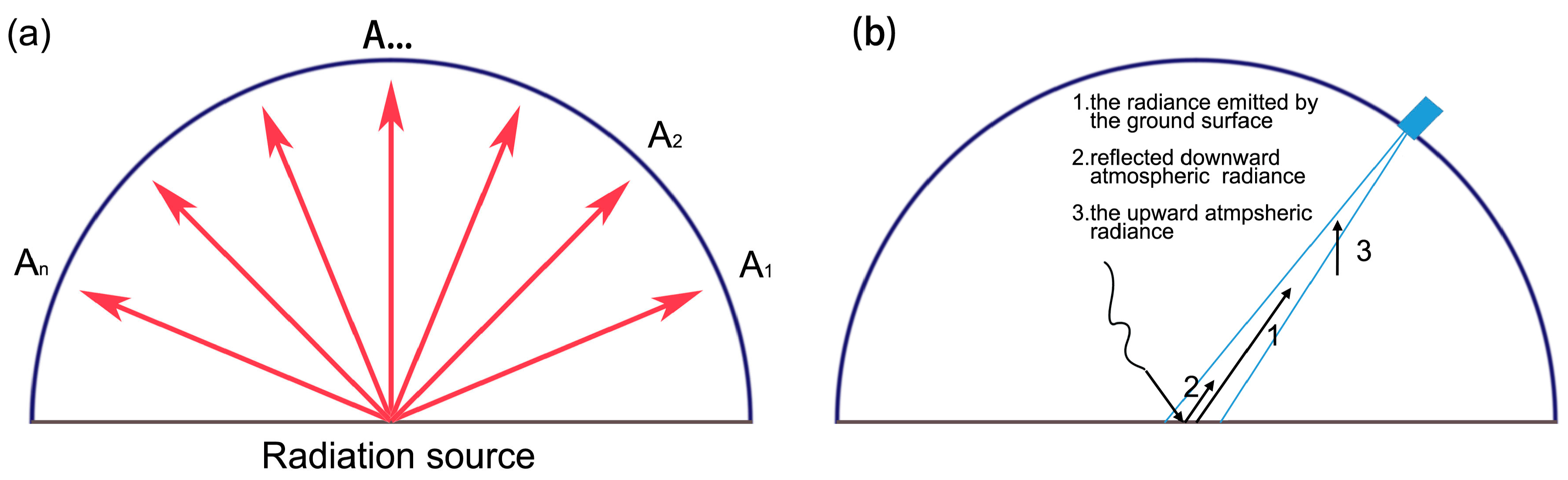
2.1.1. Correction of Atmospheric Effects

An infrared (IR) thermometer measures radiant temperatures of the ground through its observations of the thermal radiance reaching the sensor. The thermal radiance reaching the thermometer sensor is not only the emittance from the ground surface but also the emittance from the air reflected by the surface. Because the ground is not a blackbody with an emissivity of 1, they have the ability to reflect the downward thermal radiance from the air. Furthermore, the air between the IR thermometer and the ground surface can also emit a certain amount of thermal radiance to the IR thermometer. Thus, when we measure the thermal radiance of the ground surface, we may have the observation expressed as follows [38]:

$$I=I_g+I_{ar}+I_a^{\uparrow }$$

(3)

where I is the total thermal radiance reaching the IR thermometer, which can be converted from the measured radiant temperature of the IR thermometer by the Planck equation; $I_g$ is the thermal emittance from the ground surface under measurement, which is the target that we aim at because it is the term that we use to determine the surface property; $I_{ar}$ is the reflected downward atmospheric emittance by the ground; and $I_a^{\uparrow }$ is the upward atmospheric emittance between the ground and the IR thermometer.

The $I_{ar}$ term is dependent on the ground emissivity and downward atmospheric emittance $I_a^{\downarrow }$, and is generally expressed as follows [38]:

$$I_{ar}=\left(1-\mathsf{\epsilon }\right)I_a^{\downarrow }$$

(4)

where $I_a^{\downarrow }$ is the downward atmospheric emittance, which is heavily dependent on the effective atmospheric mean temperature, the atmosphere vapor content, and its distribution in the profile [1,38,39]. In remote sensing, the value can be approximated as follows [38]

$$I_a^{\downarrow }=\left(1-{\tau }_{\lambda }\right)B_{\lambda }(T_a^{\downarrow })$$

(5)

where ${\mathsf{\tau }}_{\mathsf{\lambda }}$ is the atmospheric transmittance at wavelength λ, and $B_{\lambda }(T_a^{\downarrow })$ is the Planck radiance function. The sky during our experiment days was clear. We measured the air temperature near the ground surface T_a0 at each experiment site (

Table 1. Estimation of parameter A for various surfaces at the experimental sites.

Sites	Nanjing	Beijing	Yongzhou	Jiangmen	Xilinguole
Date	2 August 2015	3 July 2015	24 October 2015	29 October 2015	31 August 2015
Ta0 day (°C)	35	30	28	30	23
$(T_a^{\downarrow })$ day (°C)	26.02	21.41	19.56	21.41	14.96
$B_{\lambda }(T_a^{\downarrow })$ (W/m2)	9.7915	9.0764	8.7994	9.0764	8.1295
w (g/cm2)	2.80	2.00	2.50	2.80	1.50
τλ	0.65	0.72	0.67	0.65	0.76
Ia (W/m2)	3.4270	2.5414	2.9038	3.1767	1.9511
Iar (W/m2)	0.0857	0.0635	0.0726	0.0794	0.0488
A water	1.0092	1.0064	1.0073	1.0080	1.0057
A grass	1.0069	1.0060	1.0064	1.0072	1.0047
A concrete	1.0065	1.0057	1.0058	1.0067	1.0041
A bare soil	1.0061	1.0046	1.0055	1.0065	1.0040

). Thus we can estimate the effective downward atmospheric temperature $T_a^{\downarrow }$ for each site. Using the corresponding standard atmospheres (subtropical and mid-latitude summer) and the relationship given in Qin et al. [1] for the standard atmospheres, we estimate the $T_a^{\downarrow }$ for the sites. Accordingly we compute the magnitude of the $B_{\mathsf{\lambda }}(T_{\mathrm{a}}^{\downarrow })$ ranges for the wavelength of our IR thermometers at 8–14 μm (Table 1). According to our in-site observation during the experiment days which were clear sky, we estimated the amount of atmospheric water vapor from the corresponding standard atmospheres so that the atmospheric transmittance τ_λ can be estimated for computation of the downward atmospheric emission to correct our observed thermal radiance (Table 1).

As indicated in Equation (4), ground emissivity is an important parameter for the correction. Since we selected typical ground surfaces for the experiments, we could use the available estimates of such typical surfaces to determine the magnitude of ground emissivity in our case, which is 0.995 for water, 0.985 for grass, 0.97 for concrete, and 0.96 for bare soil. With these estimates of ground emissivity, we are able to compute the term $I_{ar}$ with Equation (4). As shown in Table 1, $I_{ar}$ was numerically estimated to be roughly 0.064–0.086 W/m², which is very small in comparison with the value of $I_g$ (generally $I_g$ = 9.32–14.01 W/m² for ground surface temperature T_S = 23–50 °C) in our experimental sites. The small portion of $I_{ar}$ in comparison with $I_g$ makes the simplification of computing the kinetic surface temperature (KST) from the measured radiant surface temperature (RST) possible. Moreover, the distance between the ground and the IR thermometer is only about 1.5 m in our case, which makes the $I_a^{\uparrow }$ item too small to be considered. Thus, we have

$$I=I_g+I_{ar}\approx A{I}_g$$

(6)

where A is a parameter, with A = (1 + $I_{ar}$/$I_g$). The magnitude of parameter A is dependent on the amount of downward atmospheric emission $I_{ar}$, which can be estimated by Equation (4). In order to simplify the correction, the average T_s was used for each surface at each site to estimate the ground emission $I_g$ in Equation (6). With this simplification, we obtained the values of parameter A for the various surfaces of the sites (Table 1). Using the parameter A and Equation (6), we are able to determine the thermal radiance of the measured ground $I_g$ from the observed I for each experimental site, which gives $I_g$ = I/A. Though this correction of observed I into the $I_g$ is not very accurate due to the above simplifications, the accuracy of the correction is high enough for our study. According to our computation, the possible error involved in the correction is expected to be <0.1%, which is quite small in comparison to the amount of the term $I_g$.

2.1.2. Emissivity Determination

The ground surface of the earth is not a blackbody. Most natural objects on the ground surface can emit only part of their potential radiant energy [40]. The direct output of temperature measurements from an IR thermometer (or a remote sensing system) can only show the radiant (apparent) temperature change in the objects under measurement. Therefore, the emissivity ε value, which is defined as the ratio between the observed radiance of the object under measurement and the emittance of a blackbody with the same kinetic temperature, must be considered in our identification of the ground surface to determine its Lambertian property. Moreover, ground emissivity is also an important factor affecting the capability of thermal emission from the ground surface under measurement [38]. To determine the true ground radiance and true kinetic ground temperature change, ground emissivity must be considered to calculate the observed radiant temperature.

Previous studies indicated that the ground emissivity has a property of variation with the viewing angles [41,42,43,44,45,46]. However, variations in the ground emissivity with the viewing angle is usually very small when the View Zenith Angle (VZA) is smaller than 60°, especially when the angle is smaller than 40° [41,44]. Schott developed a model for the incorporation of the angular emissivity of longwave radiation [47]. According to this study, the emissivity of the concrete surface (ε = 0.94) behaves roughly in a manner very close to a Lambertian surface. According to the study of Chen et al. [48], the ground emissivity of vegetation is relatively unchangeable with VZA when the Leaf Area Index (LAI) of the vegetation is above 2. In our case, the LAI of grass in the observation sites is very high and we estimated that it is over 2. Thus, we used a fixed value (0.98) of emissivity for the grass sites in our analysis of the Lambertian property of the ground surface. Though our study has a VZA between −60° and 60°, we believe that the emissivity of the experimental sites can be determined as a fixed value. This determination of a fixed value for ground emissivity that is unchangeable with VZA may not lead to significant bias in the identification of the thermal property of the ground surface under study. The four ground surfaces examined in our study are very typical: water, concrete, bare soil, and grass. The emissivities of these typical surfaces have been examined in many studies [38,40,41,42,43,44,45,46] because they are central in shaping the environmental quality of the earth’s surface.

The emissivity of water in the thermal infrared region is the highest among the materials over the ground surface and it is very close to that of a blackbody [49]. The value of water emissivity is generally estimated as 0.995 [40,49]. Thus we also used this value in this study. Urban building materials usually have an emissivity of 0.92–0.96 depending on their structure and surface colour [50,51]. A study on urban surface emissivity based on unmixed pixels [52] found that the mean emissivity of an urban building was 0.94 in the thermal range of the spectrum. In our case, the concrete surface is normal without a light colour. Thus we assume the urban building to have an emissivity value of 0.94 for the concrete surface in this study.

Fuchs and Tanner [53] believed that the emissivity of soil is related to the volumetric water content level. Mira et al. [54] stressed the importance of an accurate determination of emissivity variations in soil water content to allow for suitable temperature retrievals for sandy soils, which show the greatest levels of variation, as well as for a variety of soils with different soil textures. According to these studies, we assumed the emissivity of bare soil to be 0.96 in our study.

Idso et al. [55] determined the emissivity values of a number of different plant leaves and found emissivity values of 0.97 to 0.99. Davies and Idso [56] concluded that most canopy emissivity values likely range from 0.965 to 0.985 and argued that a value of 0.98 should be used for most radiation balance calculations. Humes et al. [57] described the reported emissivity of vegetation as follows: grass with partial cover, 0.956; shrubs with partial cover, 0.976; and shrubs with complete cover, 0.986. Labed and Stoll [58,59] measured the emissivity of grassland (≈15 cm) at 0.983 and bush (≈100 cm) at 0.994 according to their field measurements. We use an emissivity value of 0.98 for the grass surface in four of our five study sites, and for the Xilingoule site in Inner Mongolia we use the value of 0.97, due to its location in a climatically semiarid region.

2.1.3. Computing the Ground Surface Radiance from the Observed Radiant Temperatures

The output of the IR thermometers in the study is the radiant surface temperature (RST) of the ground. According to Equation (6), the observed radiance is expressed as $\mathrm{I}\approx A{I}_g$. Since the IR thermometers used in the study measured the radiant temperature of the ground surface by detecting the radiance intensity emitted from the surface and then converting the detected radiance into temperature with a blackbody emissivity (ε = 1), the radiance of the ground surface can be expressed in the form of:

$$I=B\left(RST\right)$$

(7)

where I is the observed radiance observed by the IR thermometer and B(RST) denotes the Planck equation of the observed radiance with radiant surface temperate RST. Therefore, we can derive the ground surface radiance $I_g$ from the observed radiant surface temperature as follows:

$$I_g\approx \frac{\mathrm{I}}{A}=\frac{B\left(RST\right)}{A}$$

(8)

Since the ground surface is not a blackbody and has an emissivity, we have

$$I_g=\epsilon B\left(KST\right)$$

(9)

According to Planck’s law about radiance and temperature, we obtain

$$\mathrm{KST}=\frac{c_2}{\lambda \ln \left(A\epsilon \left(e^{c_2/\lambda T_r}-1\right)+1\right)}$$

(10)

where C₂ is the second spectral constant with C₂ = 1.439 × 10⁴ μm·K, ε is the ground emissivity, and λ is the effective mean wavelength of the IR thermometer with λ ≈ 12.15 μm. On the basis of this computation, we are able to compare the difference of the observed thermal radiance ($I_g$) and the KST of the typical ground surfaces in the five experimental sites over various viewing angles to determine their thermal characteristics behavior or Lambertian properties.

2.2. Experimental Designs

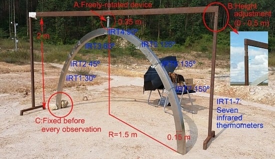
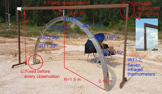
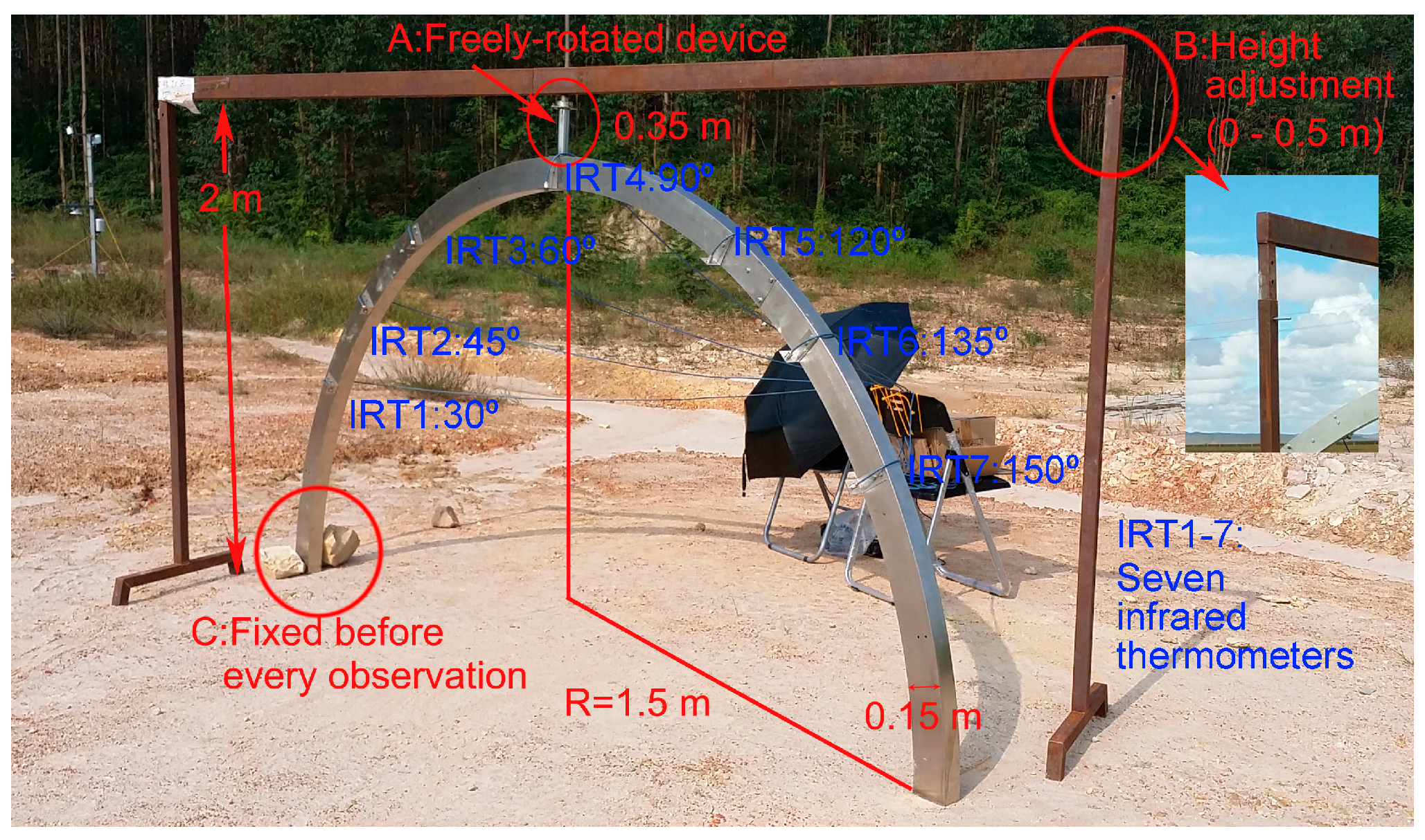
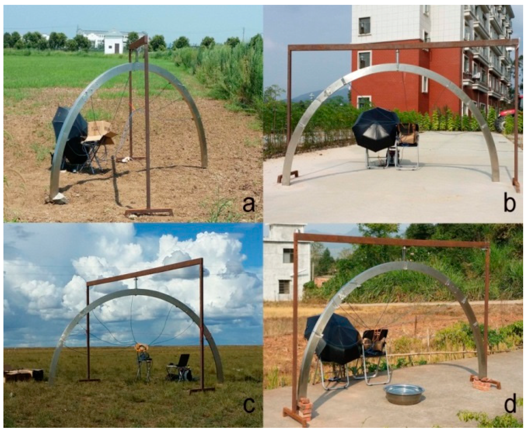
2.2.1. Experimental Observation System Design

According to the above theoretical framework for the identification of the Lambertian property of the ground surfaces, we have designed an experimental observation system to conduct the necessary measurements of the thermal radiance of typical surfaces over five experimental sites in various climate regions of China. The sites were selected to be located in different places with various climate conditions, with consideration of avoiding the possible latitude effects from solar radiation. The observation system included the following components:

Thermal infrared temperature sensor. Measurements were conducted using seven IR thermometers operating in a spectral range of 8–14 μm within the thermal spectrum. The thermometers used in study are miniature infrared sensor “MI3” from Raytek, USA. The output of the IR thermometers is RST, with a resolution of 0.1 °C and an accuracy of ±1%. With the output of the IR thermometer, we are able to calculate thermal radiance from the ground surface, using Equation (8). In order to compare the radiance from the ground in different viewing angles for the determination of the ground’s Lambertian property, we mounted the IR thermometers in 7 directions with VZAs of 30°, 45°, 60°, 90°, 120°, 135°, and 150°, respectively (Figure 2). Before observations were conducted in the field, we performed calibration of the thermal IR thermometers to keep their measurements comparable. The details of the calibration and its results are presented in Section 2.2.3. The IR thermometers can quickly (in 130 ms) respond to the thermal radiance of the target. Using the framework mounted with 7 IR thermometers for the measurement, we are able to simultaneously conduct the measurement of thermal radiance in the 7 directions, which can help us to eliminate the possible noise caused by the time difference if only one IR thermometer is used for the measurement. The output frequency of the IR thermometers is set to one record per second so that a slight change of thermal radiance can be observed through the measurements. A data logger and storage module were used to record the output of the IR thermometers.

Half-ring stainless steel plate. In order to punctually measure the thermal radiance from the exact same point of the ground surface, we designed the measurement framework in the form of a hemi-circle movable in all directions (360°) within the hemispheric space. To precisely mount the IR thermometers, we asked a factory to manufacture a framework with a half-ring stainless steel plate, using a laser cutting technique to accurately make the plate into a semicircular shape to fix the IR thermometers. The IR thermometers were installed on a freely rotated plate so that slight adjustment can be done for precise measurement. In order to minimize the possible effects from the steel framework to the IR thermometers, a plastic pipe was used for each of the IR thermometers to mount on the steel framework so that the heat from the steel can be thermally isolated to not affect the thermometers. For the convenience of transportation among different experimental sites, the framework was designed in different parts that can be assembled at the sites. Specifically, the half-ring plate was designed to be three equal parts. In each experimental site, the framework was fixed to ensure its stability for the measurements.

Iron stand. In order to avoid the possible effects from the frameworks on the measurement, an iron stand was designed to fix the IR thermometers. To be able to place the iron stand on different ground surfaces, height adjustment holes on both sides of the iron stand were designed. We drilled holes spaced 5 cm apart into the iron pipe over a total area length of approximately 60 cm. The total elongation value reached 50 cm. In the joint of the half-ring fixed plate and iron stand, a freely rotating device was designed to ensure that we could adjust the plate to the right location according to the actual observation conditions. The iron stand was assembled using four parts to facilitate transport and assembly.

A computer and different software programs were also used in the experiments. In each experimental site, the framework was set up so that the observation plate was to face the direction of solar radiation to minimize possible effects from the surrounding terrain and the shadows of the framework.

2.2.2. Experimental Sites and Period

Five experimental sites were selected for this study. These five sites were located in typical climate regions in China. The Latitude difference was 23°10′ between the northernmost site, Xilinguole in North China, and the southernmost site, Jiangmen in South China. At each site, four typical ground surfaces were selected for the experiments to observe thermal emissions: concrete, bare soil, grass, and water. In order to have a representative of the surface type in the region, the sampling site cannot be too small. Thus, we selected the area of at least 10 m² with a homogeneous surface as the sampling site except for the water surface, in which a big pan with water was used for the measurements.

For the sites selected for observation, the concrete surfaces had the simplest features among the four typical ground surfaces and hence were easily selected. Soils and grasses were more complicated to select because of their obvious spatial heterogeneity. Bare soils were characterized by different clod sizes at different sites. As to the grass, there are obvious differences in such factors such as species, leaf density, and so on, which would directly affect the consistency of the surface selected as the sample site. Furthermore, because our observation system is not very suitable for installing over natural water bodies for the observation, we altered the experimental observation over the water surface by using a water pan filled with water to represent the water surface in the sampling site. Water was in the pan with 60 cm in diameter and 20 cm in depth. Figure 3 shows the four types of observed ground surfaces.

To obtain comparable results, measurements were conducted over approximately half an hour for each surface type at the site so that the effects of different measurement periods could be minimized. We collected measurements at a time interval of 1 s for half an hour, meaning that we obtained a dataset with at least 1800 records for each observation. In order to compare with the possible effects from solar radiation, measurements were conducted at each site during the day and the following night (

Table 2. Measurement periods for the 20 sites.

Style	Measurement Time	No.	Style	Measurement Time	No.
Concrete	11:00–11:30, 4 July 2015	C1Day	Soil	16:10–16:40, 9 July 2015	S1Day
	22:00–22:30, 3 July 2015	C1Night		00:30–01:00, 10 July 2015	S1Night
	16:40–17:10, 1 August 2015	C2Day		11:10–11:40, 2 August 2015	S2Day
	22:00–22:30, 1 August 2015	C2Night		20:10–20:40, 2 August 2015	S2Night
	14:20–14:50, 1 September 2015	C3Day		16:20–16:50, 31 August 2015	S3Day
	22:45–23:15, 1 September 2015	C3Night		20:50–21:20, 31 August 2015	S3Night
	13:10–13:40, 25 October 2015	C4Day		14:00–14:30, 24 October 2015	S4Day
	21:30–22:00, 25 October 2015	C4Night		20:00–20:30, 24 October 2015	S4Night
	15:00–15:30, 29 October 2015	C5Day		11:00–11:30, 28 October 2015	S5Day
	21:00–21:30, 29 October 2015	C5Night		20:30–21:00, 27 October 2015	S5Night
Grass	10:30–11:00, 7 July 2015	G1Day	Water	09:30–10:00, 9 July 2015	W1Day
	22:00–22:30, 7 July 2015	G1Night		23:40–00:10, 9 July 2015	W1Night
	10:40–11:10, 4 August 2015	G2Day		11:00–11:30, 20 September 2015	W2Day *
	21:30–22:00, 3 August 2015	G2Night		23:30–24:00, 19 September 2015	W2Night*
	15:00–15:30, 31 August 2015	G3Day		16:50–17:20, 1 September 2015	W3Day
	21:35–22:05, 31 August 2015	G3Night		20:20–20:50, 1 September 2015	W3Night
	11:00–11:30, 25 October 2015	G4Day		15:10–15:40, 25 October 2015	W4Day
	21:30–22:00, 24 October 2015	G4Night		20:20–20:50, 25 October 2015	W4Night
	11:00–11:30, 29 October 2015	G5Day		11:00–11:30, 30 October 2015	W5Day
	20:00–20:30, 28 October 2015	G5Night		20:00–20:30, 29 October 2015	W5Night

* Because of a loss of W2 data, we conducted the observations again, and slight differences in the observation date sequence were observed.

).

Table 2 shows the specific observation times and areas used. C, S, G, and W denote the concrete site, bare soil site, grass site, and water site, respectively. Arabic numerals 1, 2, 3, 4, and 5 denote the Beijing (BJ), Nanjing (NJ), Xilinguole (XLGL), Yongzhou (YZ), and Jiangmen (JM) stations, respectively.

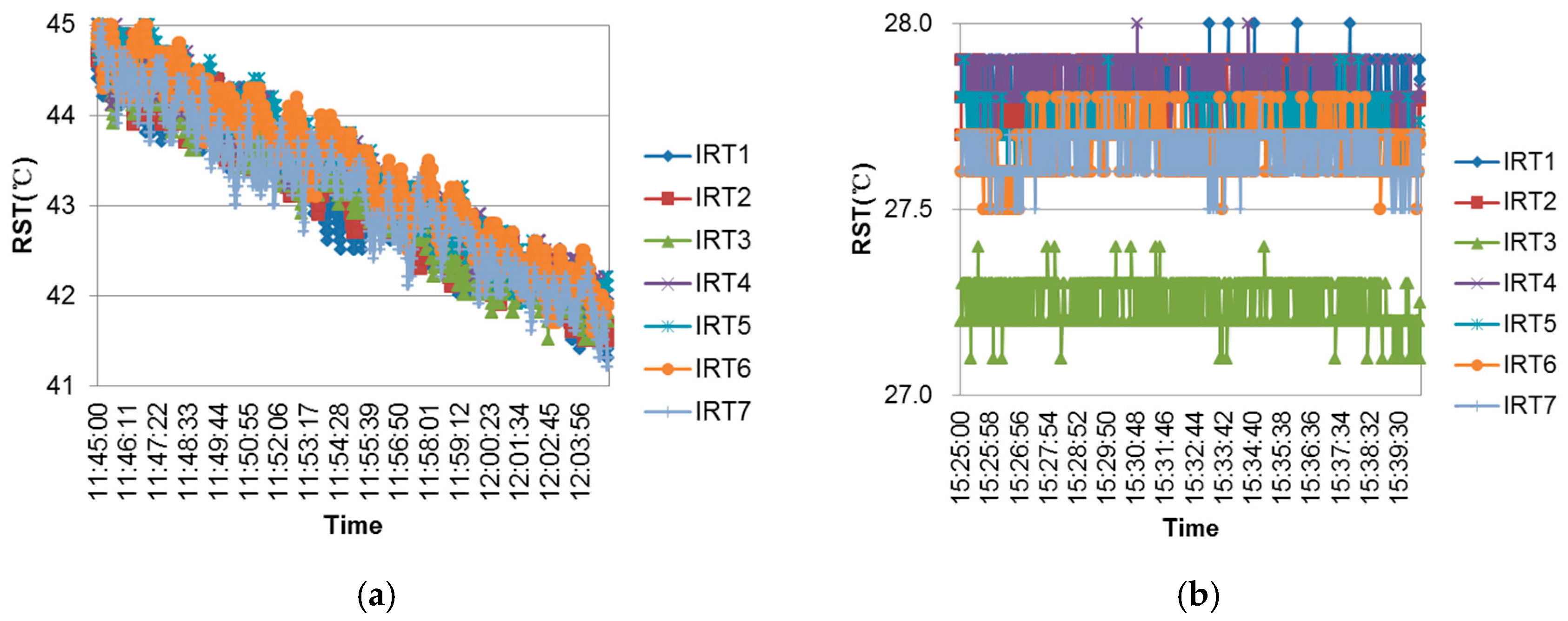
2.2.3. Calibration of the IR Thermometers

Generally, slight internal errors may occur among the seven IR thermometers when measuring the same volume of thermal emissions. In our study, seven IR thermometers were mounted at different VZAs to simultaneously measure the thermal emissions from the same ground surface point in different directions. To ensure the accuracy of the measurements, we had to calibrate the IR thermometers before using them to conduct the measurements at the experimental sites. Two steps were involved in the calibration of the IR thermometers: selecting a thermometer as a base to calibrate the others and determining the calibration constants for each thermometer. Thus, we first tested the consistency among the thermometers by using another independent handhold thermometer to measure different ground objects, including water, bare soil, and green vegetation leaves. We then selected the thermometer with the closest value to the handhold thermometer and labeled it as IRT1. The other six thermometers were numbered from IRT2 to IRT7.

To determine the calibration constants for the thermometers, we selected water as the measurement object. This is because water has very good thermal conductivity and we can rationally assume that the kinetic temperature over the water surface would be homogeneous to meet the requirement of the calibration measurements. Two temperature conditions were considered for the calibration: high and low. For the high temperature condition, we heated the water to above 45 °C to meet the potential temperature level of the ground surface during the hot summer season. We put the hot water into a container for the measurement. When the water in the container showed a stable surface, we used a device to hold the thermometers together to point at a small area of the water surface over the container at ~0.5 m to measure its temperature. The measurement was conducted in our laboratory for ~20 min, i.e., from 11:45 to 12:05.

Figure 4a shows the measurement results of the seven IR thermometers over the water at the high temperature condition. It can be seen in Figure 4a that the thermometers have very similar responses to the thermal emission from the water. The measured temperatures gradually decreased as the water cools down with time. In spite of slight fluctuation among the measurements, their average temperature difference from IRT1 can be used as the calibration constants for IRT2–IRT7 under the high temperature condition. After 2 h, the water was ultimately cooled down to normal temperature at ~27 °C, and we conducted the calibration measurement under the low temperature condition for ~25 min, i.e., from 15:25 to 15:47. The results are shown in Figure 4b, which indicated that the measurements were quite stable for each thermometer at the low temperature condition in spite of the slight differences among them, which can be used as the exact calibration constants after averaging. Finally, we determined the calibration constants for the seven IR thermometers used in the study as shown in

Table 3. Calibration constants for the 7 thermometers used in the study.

	IRT1	IRT2	IRT3	IRT4	IRT5	IRT6	IRT7
10–30 °C	0	−0.06	−0.60	−0.03	−0.11	−0.17	−0.20
30–50 °C	0	0.03	−0.03	0.26	0.28	0.30	0

.

2.3. Statistical Analysis Methods

Since a Lambertian surface has the property of homogeneous thermal emission in all directions within the hemispheric space, a comparison has been carried out with the measurement outputs from the various VZAs to determine whether or not the ground surface has the Lambertian property. In another words, we have to conduct statistical tests to the measurement outputs of the thermal radiance emitted from the ground surface and observed at the seven different VZAs (30°, 45°, 60°, 90°, 120°, 135°, and 150°) to see if there is, statistically, a significant difference among the observed thermal radiance from the VZAs. The statistical tests, i.e., analysis of variance (ANOVA) and Friedman tests used in the study, were conducted via SPSS (statistical package for the social sciences) software.

2.3.1. One-Way ANOVA and Friedman Test

The ANOVA test is a powerful tool for isolating the effects of different nominal variables (both separately and in combination) on a dependent variable. The analytical procedure of ANOVA reveals the proportion of variation in a dependent variable that can be accounted for by variations in one or more independent variables [60]. The Friedman test is a nonparametric test method to detect differences between several related groups. These analysis methods have been used in many studies including both geography and remote sensing [61,62,63].

The homogeneity of variance is an important premise of ANOVA. A test of the homogeneity of variance, the Levene test, was conducted before ANOVA. If the variance was homogeneous, one way ANOVA was used. When the variance was not homogeneous, a nonparametric Friedman test was conducted. In our study, the one-way ANOVA method and Friedman test were used to test how variations in the observed VZAs affected the observation results of the thermal radiance emitted from the same ground surface under measurement.

2.3.2. Post Hoc Multiple Comparison Tests

One-way ANOVA and Friedman tests are only able to show the occurrence of at least one difference among the various groups, implying that they are not able to identify the difference among any pairs of the groups. Thus, once differences were observed among the means, post hoc range tests and pairwise multiple comparisons need to be conducted so that the differences between each pair of the groups or any two-angle combinations in our study can be revealed.

The least significant difference (LSD) tests are commonly used as multiple comparison test methods [64,65] and are suitable for our study because we examined 7 groups and 21 pairwise comparisons. Applying the LSD pairwise multiple comparison test method is equivalent to conducting multiple individual t-tests between all pairs of groups. Tukey’s honest significant difference test is another commonly-used multiple comparison test method [61,66,67] , which uses studentized range statistics to draw pairwise comparisons between groups and sets the experiment-wise error rate to the error rate for all pairwise comparisons. The LSD is less restrictive. Thus, a statistically significant result can be easily obtained. As a contrast, Tukey’s method is more conservative. To improve the accuracy of our results, these two commonly-used test methods were used in our study. When the variances were unequal, the Tamhanes T2 test method (conservative pairwise comparison test based on a t-test) was used to draw pairwise multiple comparisons.

3. Results and Analysis

3.1. Test for Radiance in Different Directions

3.1.1. Significant Difference Test Results

About half of the radiance values observed for our study sites were tested via an ANOVA, and the remaining groups with unequal variances were examined via the Friedman test method.

Table 4. Analysis of variance and Friedman test of the seven directions. (Sig. 1: P of the homogeneity of variance test; Sig. 2: P of the F test (one-way ANOVA); Sig. 3: P of the Friedman test; HOV: homogeneity of variance; SD: significant difference; BJ, NJ, XLGL, YZ and JM denote Beijing, Nanjing, Xilinguole, Yongzhou, and Jiangmen, respectively; D and N denote day and night).

		Concrete-D	Concrete-N	Grass-D	Grass-N	Soil-D	Soil-N	Water-D	Water-N
BJ	Sig. 1	0.002	0.005	0.000	0.050	0.992	0.879	0.000	0.045
	HOV	No	No	No	No	Yes	Yes	No	No
	Sig. 2	——	——	——	——	0.000	0.000	——	——
	Sig. 3	0.000	0.000	0.000	0.000	——	——	0.000	0.000
	SD	Yes	Yes	Yes	Yes	Yes	Yes	Yes	Yes
NJ	Sig. 1	0.603	0.618	0.888	0.000	0.193	0.642	0.036	0.001
	HOV	Yes	Yes	Yes	No	Yes	Yes	No	No
	Sig. 2	0.000	0.000	0.000	——	0.000	0.000	——	——
	Sig. 3	——	——	——	0.000	——	——	0.000	0.000
	SD	Yes	Yes	Yes	Yes	Yes	Yes	Yes	Yes
XLGL	Sig. 1	0.851	0.260	0.000	0.000	0.736	0.006	0.002	0.001
	HOV	Yes	Yes	No	No	Yes	No	No	No
	Sig. 2	0.005	0.000	——	——	0.974	——	——	——
	Sig. 3	——	——	0.000	0.000	——	0.000	0.000	0.000
	SD	Yes	Yes	Yes	Yes	No	Yes	Yes	Yes
YZ	Sig. 1	0.021	0.127	0.007	0.000	0.000	0.991	0.000	0.120
	HOV	No	Yes	No	No	No	Yes	No	Yes
	Sig. 2	——	0.000	——	——	——	0.000	——	0.000
	Sig. 3	0.000	——	0.000	0.000	0.000	——	0.000	——
	SD	Yes	Yes	Yes	Yes	Yes	Yes	Yes	Yes
JM	Sig. 1	0.000	0.415	0.730	0.462	0.118	0.692	0.011	0.416
	HOV	No	Yes	Yes	Yes	Yes	Yes	No	Yes
	Sig. 2	——	0.000	0.000	0.000	0.000	0.000	——	0.000
	Sig. 3	0.000	——	——	——	——	——	0.000	——
	SD	Yes	Yes	Yes	Yes	Yes	Yes	Yes	Yes

shows the results of the statistical tests of the thermal emission difference among different viewing angles. The results indicate that the difference in radiance was found to be statistical significance among the seven viewing angles for most observed sites (39 of 40 groups). This implies that the selected ground surfaces under study may not behave with the Lambertian property in the thermal infrared region. Moreover, we also found that the difference of observed thermal radiance is most obvious in the grass among the selected surfaces. This is probably attributed to the roughness of the grass since the roughness of the ground surface may have important effects on the observation of its thermal emission from different viewing angles.

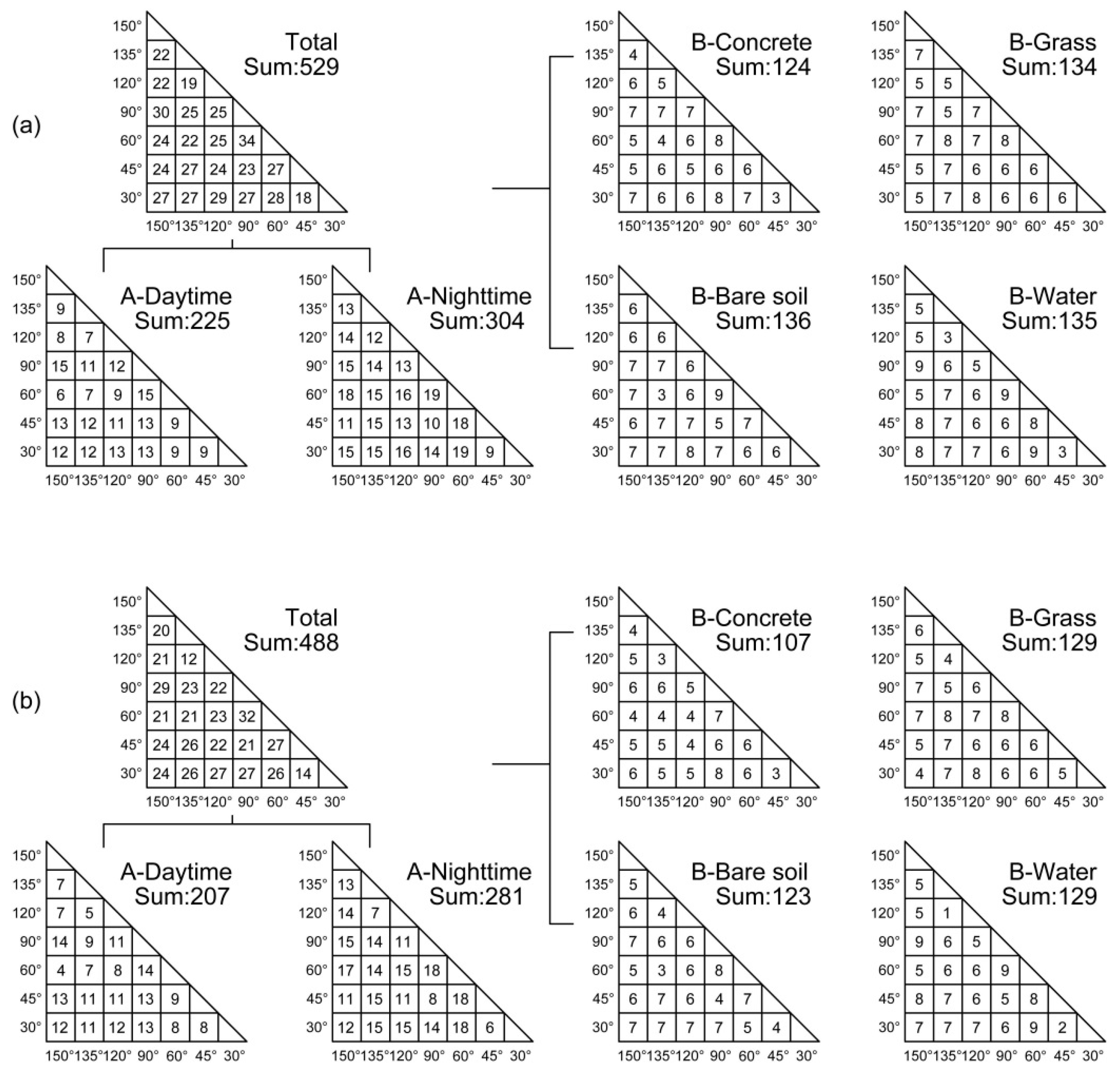
3.1.2. Post Hoc Multiple Comparison Tests

The above test results show that the radiance values observed in the seven directions present significant differences. However, the results only show that at least one difference occurred among the various groups, and they do not identify the groups that are different. To determine the difference in radiation values among all directions, post hoc multiple comparison tests were conducted. We conducted post hoc multiple comparison tests based on the LSD and Tukey’s significant difference tests and the Tamhanes T2 test approach.

Figure 5 shows the results of the multiple comparison tests. Significant differences were found between every pair of the seven angles. Our multiple comparison tests of every two directions show that significant differences occur between two directions in all seven cases but are less common for concrete surfaces than for the other three types of land surfaces (Figure 5), because the concrete surfaces have the smallest roughness. The multiple comparison tests also show that the significant differences that occur between two directions are less common during the daytime than the nighttime. These results may have been related to the effect of solar radiation and the heterogeneity of the ground surface. In the daytime, the angular variation in the ground surface radiance may be caused by the heterogeneity of the ground surface and the solar irradiance received by different parts of the sampling sites. During the night, the angular variation in the ground surface radiance was only caused by the heterogeneity of the ground surface. The significant differences that occur between every two directions are less common during the daytime than the nighttime because the solar radiation more strongly affected the radiance emitted from different angles than the heterogeneity of the ground surface. This created less significant differences in the radiance from each pair of angles.

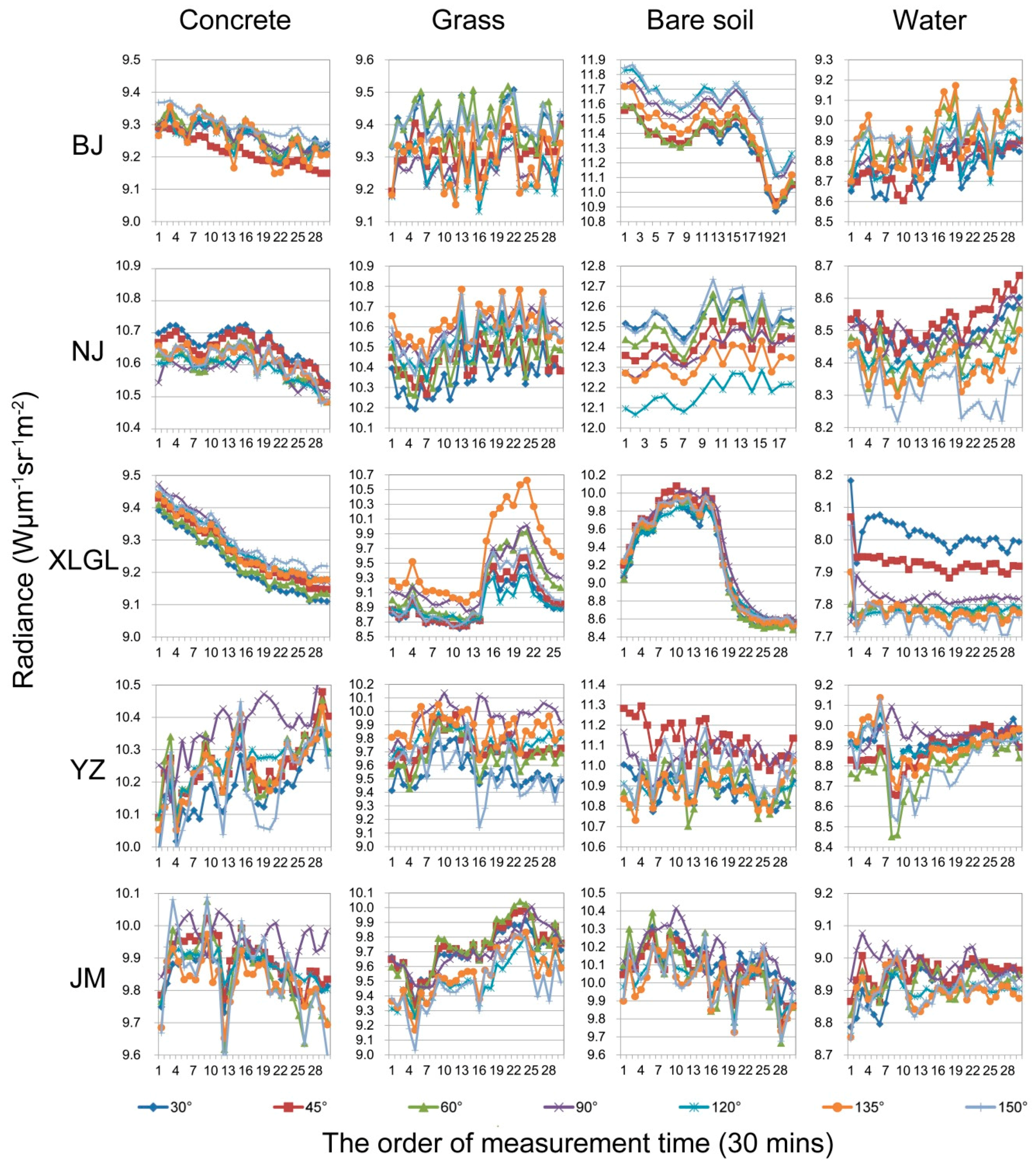
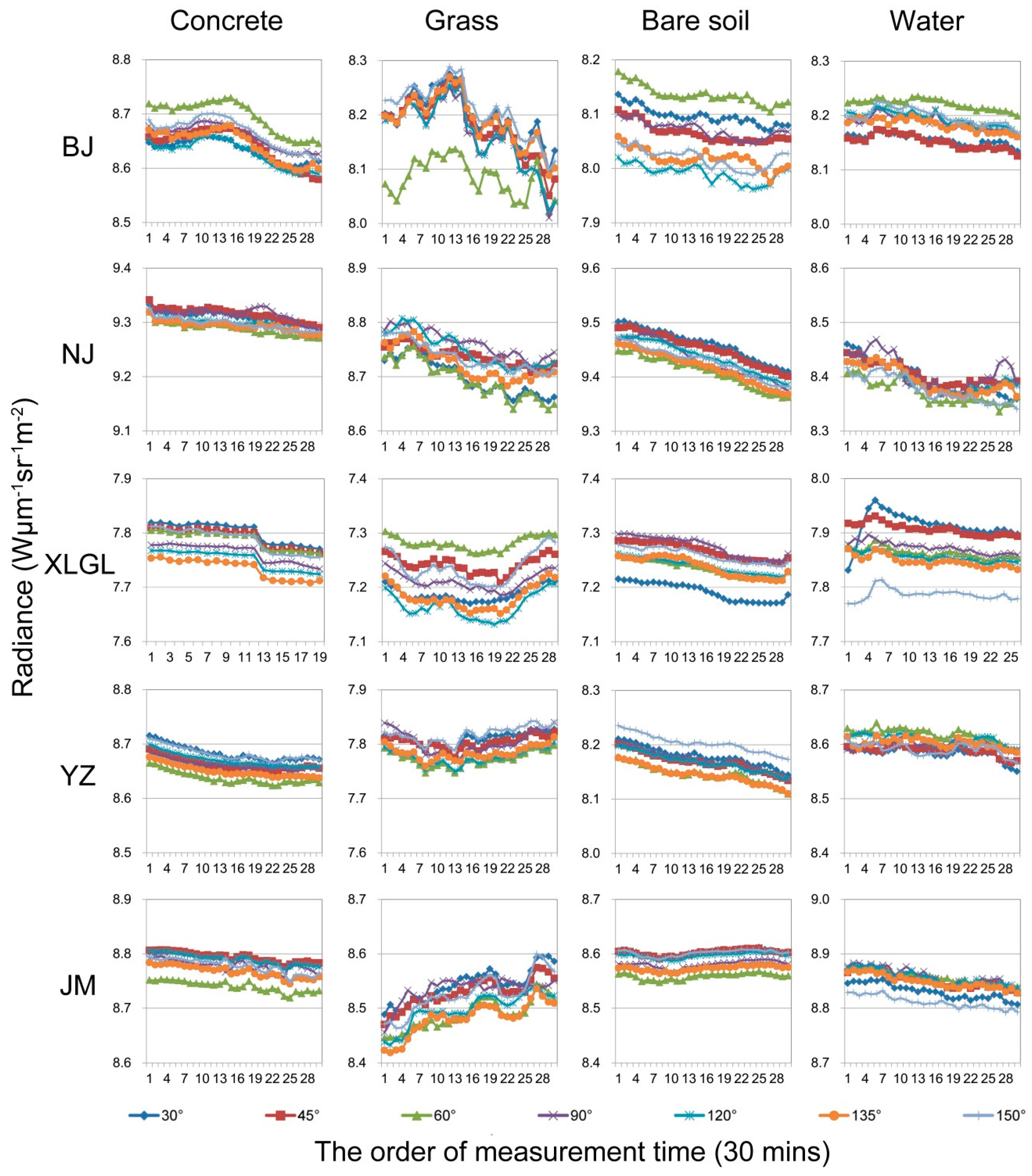
3.2. Radiance Directionality Change

Figure 6 shows the radiance change that occurs over 30 continuous minutes of measurement during the daytime at the 20 sites. During the observation period, changes were observed in the radiance of the seven observed angles and differences in radiance were observed among the angles. The radiation difference was also different across the four types of ground surfaces. Grass and bare soil presented the highest radiance directional difference. These two types of ground surfaces present relatively significant radiance differences, and the radiance values of the seven directions include a fluctuating region exceeding a value of 0.5 W·μm⁻¹·sr⁻¹·m⁻² followed by water (~0.5 W·μm⁻¹·sr⁻¹·m⁻²). The concrete surface generated the smallest fluctuating region (less than 0.5 W·μm⁻¹·sr⁻¹·m⁻²) (Figure 6) because of the varying physical and geometric characteristics of these four types of ground surfaces. In YZ and JZ, the material heterogeneity of the concrete surface may have been larger than that in the other three concrete sites, which caused the results to differ. We knew that the water surfaces have relatively lower surface roughness, while Figure 6 shows a larger variation in the radiance of the water surface. It may be due to two reasons: (1) Although we have made great efforts to ensure that the observed target of IRT in these different angles is the water (such as choosing a certain area and height of the basin according to the detailed parameters of thermometers), the basin may have still affected our observations. (2) The other reason may be the fluctuations of the water surface, which make the different thermal emissions observed from different directions.

Many studies found that different levels of solar irradiance received by different parts of objects cause radiance directionality [7,12,17]; therefore, radiance directionality is influenced by direct sunlight irradiance during the daytime. For higher roughness observation objects, such as grass and bare soil, the radiance directionality caused by solar irradiance is more obvious. A small difference in radiance values between the concrete and water was observed because of their relatively smooth surfaces. However, the results in Figure 6 do not show any obvious radiance change trend caused by the view angle. For example, the radiance of the seven VZAs for the bare soil site in Beijing exhibits the following relationship: 120° > 150° > 90° > 135° > 30° $\approx$ 45° $\approx$ 60°. However, this order only appeared at this site.

Figure 7 shows the radiance change values for 30 continuous minutes at night for 20 sites. As shown in this figure, the radiance differences for different angles at night were much less significant than they were during the day. During the observation period, seven directions of radiance present a fluctuating region of less than 0.3 W·μm⁻¹·sr⁻¹·m⁻². In most of the sites, this range is roughly 0.1 W·μm⁻¹·sr⁻¹·m⁻². The radiance of directions in the grass sites present a larger fluctuating region than the other three.

A comparison of Figure 6 and Figure 7 shows that the radiance difference between the seven directions is clear during the day but much less significant at night. This result is consistent with other studies [32]. We also found that the radiance of the seven directions stayed relatively stable at night but fluctuated throughout the experiments performed during the day. This finding implies that solar radiation affected not only the surface radiance value but also radiance anisotropy. According to the results of the above statistical test, the radiance differences during the night are smaller than those during the daytime, although significant differences in the radiance appeared over different observed angles during both the day and night.

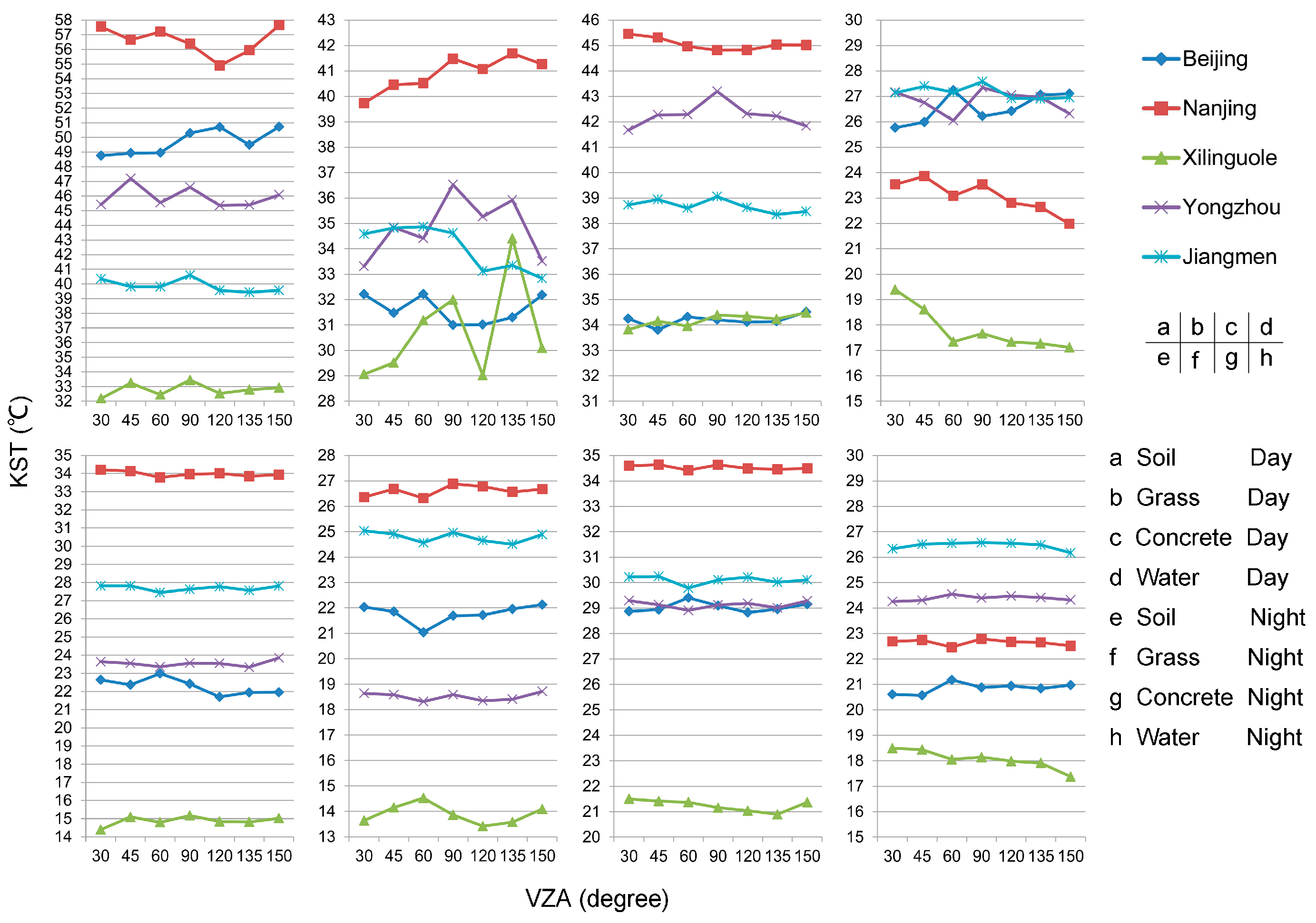
3.3. KST Directionality Change

To determine the thermal characteristics of the typical ground surfaces, the KST of the typical ground surfaces in the five experimental sites over various viewing angles were calculated (Figure 8).

Figure 8 shows the KST changes at the 20 sites, including four typical ground surfaces at five stations. KST differences existed among the different zenith angles. During the day, the KST differences among the four surface patterns were obvious. Grass had the highest KST difference in every site with a value of 2–5 °C (Figure 8b), followed by soil and water (2–3 °C) (Figure 8a,d). The concrete had the lowest KST difference between the different angles, approximately 1–2 °C (Figure 8c). During the night, the KST differences were not obvious and were mostly about 0.5–1 °C (Figure 8e–h). No fixed variation trends with the viewing angle were present.

3.4. Radiance and KST Directional Differences with Surface Roughness

The objects observed in this study are natural ground surfaces. Therefore, it is very difficult to have observation sites with identical characteristics over the same types of ground surfaces. We can logically assume that the characteristic differences between the different sites are negligible for the concrete and water surfaces due to their relative homogeneous features over the surface. For the sites of bare soil and grass, the characteristic differences are relatively obvious. According to the clod size of the bare soils, we divided the surface roughness of five bare soil sites into three categories: high roughness soil (diameter of the clod size is roughly 1–2 cm), medium roughness soil (diameter of the clod size is roughly 0.5–1 cm), and low roughness soil (diameter of the clod size is less than 0.5 cm). Soil sites S1 (BJ) and S2 (NJ) belong to the high roughness soil category. Soil site S4 (YZ) exhibits moderate roughness, and soil sites S3 (XLGL) and S5 (JM) exhibit low roughness. Our bare soil roughness classification is different from that of Zhang [27], and the three levels of soil roughness (high roughness soil, moderate roughness soil, and low roughness soil) belong to the low roughness soil category according to Zhang’s study.

Grass sites were also divided into three levels of roughness. Grass site G1 (BJ) and grass site G2 (NJ) are trimmed lawn sites with high leaf area coverage. The roughness levels in these two sites belong to the low roughness class. Grass sites G3 (XLGL), G4 (YZ), and G5 (JM) belong to the natural growth grass class. Greater differences between grass heights in a site increase the grass surface roughness. Among the three natural growth grass sites, G3 has the highest roughness, and grass grows more sparsely in this site. Figure 9 shows the five soil sites and five grass sites.

The roughness levels in the five bare soil sites exhibit the following relationship: S1 ≈ S2 > S4 > S3 ≈ S5. Figure 6 and Figure 8 show that the radiance changes and the average KST changes calculated across the five sample sites exhibit the following relationship: S2 > S1 > S4 > S5 > S3. S1 and S2 present the highest roughness values and the largest differences in radiance across the seven directions. S4 and S5 present minor radiance differences because of the presence of low roughness levels. Figure 6 and Figure 8 show that the radiance changes and the average KST changes calculated across the five grass sample sites are in the following order: G3 > G4 > G5 > G2 > G1. We also found that the roughness of these five grass sites adheres to the following pattern: G3 > G4 ≈ G5 > G1 ≈ G2. Thus, we concluded that the radiance differences were positively correlated with the surface roughness.

Although the examined sites were divided into three categories according to the roughness levels, the identified roughness values were still small. For certain studies, the roughness of observed targets is larger, thus revealing a complex three-dimensional structure. Therefore, certain regularities may be found in specific directions. Chen et al. [68] found that crops are frequently planted in rows, which may create large differences between sunlit and shaded soil surfaces and foliage temperatures, thus causing pixels to vary in their azimuth orientations and generating changes in the radiant directionality of row crops in the zenith and azimuth orientations. This regularity can be used to study targets rather than simply assuming the presence of Lambert bodies. Furthermore, in certain studies, assuming that observed targets are Lambert bodies will not exacerbate the errors.

4. Discussion

4.1. Effect of FOV on Observed Thermal Emission

Rough ground may have different planes when viewed from different directions. These planes may behave with different thermal properties due to their differences in facing solar radiation. In this case, one might observe thermal differences when viewing from different directions, which has been termed as FOV effects [6,7,8]. Such phenomena usually occur in city environment because buildings in the city have different faces which may have obvious differences in temperature as a result of sunshine. In sparse forest, the tree canopy may not completely cover the ground and some trees may be taller than others, which consequently may lead to the tree canopy having relatively higher temperature on the side facing the sunshine than the other side backing the sunshine. Coarse bare soil in the field may also behave with similar thermal differences [27]. This difference in temperature as a result of different solar radiation has been described as a directional rule for thermal emission [6,7,8,21,27]. Our results from the experiments indicated that no directional rule was observed in the relatively rough ground surfaces, i.e., grass. Instead we observed some temperature differences among different viewing angles. Since this difference is not regular, we think that it may be due to the random distribution of the grass leaves in the 3-dimensional space, which is quite different from the regular arrangement of building faces in the city environment or the tree canopy in a sparse forest. Moreover, the distance between our IR thermometers and the ground surface was only 1.5 m. The short distance of observation may cause the thermometer to focus on a relative small ground surface, which consequently may lead to bias in the observation. As a result, we obtained some difference in their thermal emissions. In this case, the observed difference of thermal emission over the rough surface does not deny its Lambertian property. This is especially true in an urban environment. The radiance difference was also obvious in different directions, due to their facing to the sunshine or not [35].

4.2. Lambertian Property of Thermal Infrared Regions and Reasonable Assumptions

Our statistical test reveals a significant radiance difference between different angles, indicating that the earth’s surface does not present Lambertian characteristics in thermal infrared regions that can be observed via thermal remote sensing. The experimental results of this study also reveal that the ground surface tends to behave with a Lambertian property when the roughness of the surface is small.

For remote sensing applications, specific analyses should be conducted in conjunction with the use of specific research objects, satellite observation times, and research goals before a proper Lambertian hypothesis is developed. Sometimes, objects are located in an urban region with tall buildings, and mountains and other observed targets have complex three-dimensional structures. Assuming that the earth’s surface is a Lambert body that can introduce errors, the influence of FOV effects, hotspot effects, and component temperatures should be considered in certain instances. We should consider such effects comprehensively to mitigate the errors caused by them. For example, “component temperatures” must be considered in the case of very low spatial resolution remote sensing images. Spatial and temporal thermal anisotropy methods have been studied, and many algorithms and models have been proposed as methods of performing angular corrections to LST or extracting component temperatures from multi-angular remotely sensed data [13,19,23].

5. Conclusions

The presence of Lambertian surfaces represents an important assumption for the construction of thermal radiance transfer equations for the remote sensing of ground surface temperatures. Four typical ground surfaces were selected for our experiments to observe thermal emissions: bare soil, grass, water, and concrete. Our experiments were conducted in five different regions of China. Down-welling atmospheric emissions were considered for the correction of observed radiance values to ground surface radiance values in our experiments. What we wanted to demonstrate is whether or not the ground surfaces in the above typical patterns behave with a Lambertian property in the thermal infrared region (8–14 μm), to have an equal ability of emission into all directions for observation. The results of our experiments indicate that the selected ground surfaces, especially the grass and the bare soil, may not behave with the Lambertian property in thermal infrared region. This is probably attributed to the roughness of the selected surface, because we found that roughness is an important factor affecting the observed magnitude of thermal emission from different directions of the ground surface under study. Therefore, whether or not a terrestrial surface can be assumed to be a Lambertian surface should be based on their geometric structure. When the surface is relatively smooth, we can say that it is close to the Lambertian property regarding thermal emission. On the other hand, we also understand that many factors may play important roles in affecting the thermal emission of the ground surface to the hemispheric space and our experiments are still lacking consideration of the possible effects from all these factors. Therefore, great effort it still needed to continue the work in identifying the Lambetian property of the ground surfaces of the Earth, and in particular, precise experiments of observation and the selection of as many typical ground surfaces as possible.

References

1. Qin, Z.; Karnieli, A.; Berliner, P. A mono-window algorithm for retrieving land surface temperature from Landsat TM data and its application to the Israel-Egypt border region. Int. J. Remote Sens. 2001, 22, 3719–3746. [Google Scholar] [CrossRef]
2. Hook, S.J.; Gabell, A.R.; Green, A.A.; Kealy, P.S. A comparison of techniques for extracting emissivity information from Thermal Infrared data for geologic studies. Remote Sens. Environ. 1992, 42, 123–135. [Google Scholar] [CrossRef]
3. Qin, Z.; Dall’Olmo, G.; Karnieli, A.; Berliner, P. Derivation of split window algorithm and its sensitivity analysis for retrieving land surface temperature from NOAA—advanced very high resolution radiometer data. J. Geophys. Res. 2001, 106, 22655–22670. [Google Scholar] [CrossRef]
4. McMillin, L.M. Estimation of sea surface temperatures from two infrared window measurements with different absorption. J. Geophys. Res. 1975, 80, 5113–5117. [Google Scholar] [CrossRef]
5. Wang, F.; Qin, Z.; Song, C.; Tu, L.; Karnieli, A.; Zhao, S. An improved mono-window algorithm for land surface temperature retrieval from Landsat 8 thermal infrared sensor data. Remote Sens. 2015, 7, 4268–4289. [Google Scholar] [CrossRef]
6. Zhan, W.; Chen, Y.; Voogt, J.A.; Zhou, J.; Wang, J.; Ma, W.; Liu, W. Assessment of thermal anisotropy on remote estimation of urban thermal inertia. Remote Sens. Environ. 2012, 123, 12–24. [Google Scholar] [CrossRef]
7. Lagouarde, J.P.; Hénon, A.; Kurz, B.; Moreau, P.; Irvine, M.; Voogt, J.; Mestayer, P. Modelling daytime thermal infrared directional anisotropy over toulouse city centre. Remote Sens. Environ. 2010, 114, 87–105. [Google Scholar] [CrossRef]
8. Lagouarde, J.P.; Hénon, A.; Irvine, M.; Voogt, J.; Pigeon, G.; Moreau, P.; Masson, V.; Mestayer, P. Experimental characterization and modelling of the nighttime directional anisotropy of thermal infrared measurements over an urban area: Case study of Toulouse (France). Remote Sens. Environ. 2012, 117, 19–33. [Google Scholar] [CrossRef]
9. Lagouarde, J.P.; Irvine, M. Directional anisotropy in thermal infrared measurements over toulouse city centre during the CAPITOUL measurement campaigns: First results. Meteorol. Atmos. Phys. 2008, 102, 173–185. [Google Scholar] [CrossRef]
10. Lagouarde, J.P.; Moreau, P.; Irvine, M.; Bonnefond, J.M.; Voogt, J.A.; Solliec, F. Airborne experimental measurements of the angular variations in surface temperature over urban areas: Case study of Marseille (France). Remote Sens. Environ. 2004, 93, 443–462. [Google Scholar] [CrossRef]
11. Voogt, J.A. Assessment of an urban sensor view model for thermal anisotropy. Remote Sens. Environ. 2008, 112, 482–495. [Google Scholar] [CrossRef]
12. Ren, H.; Yan, G.; Liu, R.; Nerry, F.; Li, Z.L.; Hu, R. Impact of sensor footprint on measurement of directional brightness temperature of row crop canopies. Remote Sens. Environ. 2013, 134, 135–151. [Google Scholar] [CrossRef]
13. Zhan, W.; Chen, Y.; Zhou, J.; Li, J. An algorithm for separating soil and vegetation temperatures with sensors featuring a single thermal channel. IEEE Trans. Geosci. Remote Sens. 2011, 49, 1796–1809. [Google Scholar] [CrossRef]
14. Liu, Q.; Yan, C.; Xiao, Q.; Yan, G.; Fang, L. Separating vegetation and soil temperature using airborne multiangular remote sensing image data. Int. J. Appl. Earth Obs. Geoinf. 2012, 17, 66–75. [Google Scholar] [CrossRef]
15. Liu, Q.; Chen, L.; Liu, Q.; Xiao, Q. A radiation transfer model to predict canopy radiation in thermal infrared band. J. Remote Sens. 2003, 7, 161–167. [Google Scholar]
16. Otterman, J.; Susskind, J.; Brakke, T.; Kimes, D.; Pielke, R.; Lee, T.J. Inferring the thermal-infrared hemispheric emission from a sparsely-vegetated surface by directional measurements. Bound.-Layer Meteorol. 1995, 74, 163–180. [Google Scholar] [CrossRef]
17. Yan, G.; Jiang, L.; Wang, J.; Chen, L.; Li, X. Thermal bidirectional gap probability model for row crop canopies and validation. Sci. China Ser. D Earth Sci. 2003, 46, 1241–1249. [Google Scholar] [CrossRef]
18. Yan, G.; Ren, H.; Hu, R.; Yan, K.; Zhang, W. A portable multi-angle observation system. In Proceedings of the 2012 IEEE International Geoscience and Remote Sensing Symposium (IGARSS), Munich, Germany, 22–27 July 2012; pp. 6916–6919. [Google Scholar]
19. Yu, T.; Gu, X.; Tian, G.; Legrand, M.; Baret, F.; Hanocq, J.F.; Bosseno, R.; Zhang, Y. Modeling directional brightness temperature over a maize canopy in row structure. IEEE Trans. Geosci. Remote Sens. 2004, 42, 2290–2304. [Google Scholar]
20. Li, Z.L.; Zhang, R.; Sun, X.; Su, H.; Tang, X.; Zhu, Z.; Sobrino, J.A. Experimental system for the study of the directional thermal emission of natural surfaces. Int. J. Remote Sens. 2004, 25, 195–204. [Google Scholar] [CrossRef]
21. Rasmussen, M.O.; Göttsche, F.M.; Olesen, F.S.; Sandholt, I. Directional effects on land surface temperature estimation from meteosat second generation for savanna landscapes. IEEE Trans. Geosci. Remote Sens. 2011, 49, 4458–4468. [Google Scholar] [CrossRef]
22. Lagouarde, J.P.; Ballans, H.; Moreau, P.; Guyon, D.; Coraboeuf, D. Experimental study of brightness surface temperature angular variations of maritime pine (pinus pinaster) stands. Remote Sens. Environ. 2000, 72, 17–34. [Google Scholar] [CrossRef]
23. Otterman, J.; Brakke, T.W.; Susskind, J. A model for inferring canopy and underlying soil temperatures from multi-directional measurements. Bound.-Layer Meteorol. 1992, 61, 81–97. [Google Scholar] [CrossRef]
24. Rasmussen, M.O.; Pinheiro, A.C.; Proud, S.R.; Sandholt, I. Modeling angular dependences in land surface temperatures from the seviri instrument onboard the geostationary meteosat second generation satellites. IEEE Trans. Geosci. Remote Sens. 2010, 48, 3123–3133. [Google Scholar] [CrossRef]
25. Yan, G.; Friedl, M.; Li, X.; Wang, J.; Zhu, C.; Strahler, A.H. Modeling directional effects from nonisothermal land surfaces in wideband thermal infrared measurements. IEEE Trans. Geosci. Remote Sens. 2001, 39, 1095–1099. [Google Scholar]
26. Yu, T.; Gu, X.; Tian, G.; Legrand, M.; Hanocq, J.F.; Bosseno, R. Analyzing the errors caused by FOV effect on the ground observations of directional brightness temperature over a row structured canopy. J. Remote Sens. 2004, 8, 443–450. [Google Scholar]
27. Zhang, R.; Sun, X.; Li, Z.L.; Stoll, M.P.; Su, H.; Tang, X. Revealing of major factors in the directional thermal radiation of ground objects. Sci. China Ser. E Technol. Sci. 2000, 43, 34–40. [Google Scholar] [CrossRef]
28. Suits, G.H. The calculation of the directional reflectance of a vegetative canopy. Remote Sens. Environ. 1973, 2, 117–125. [Google Scholar] [CrossRef]
29. Sobrino, J.A.; Caselles, V. Thermal infrared radiance model for interpreting thermal radiation from a terrestrial surface. J. Appl. Meteorol. 1990, 18, 759–763. [Google Scholar]
30. Gillespie, A.R. Spectral mixture analysis of multispectral thermal infrared images. Remote Sens. Environ. 1992, 42, 137–145. [Google Scholar] [CrossRef]
31. Weng, Q.; Fu, P.; Gao, F. Generating daily land surface temperature at Landsat resolution by fusing Landsat and MODIS data. Remote Sens. Environ. 2014, 145, 55–67. [Google Scholar] [CrossRef]
32. Sun, H.; Chen, Y.; Zhan, W.; Ma, W. Temperature diurnal change of walls and the effect on modeling urban thermal anisotropy. In Proceedings of the 2012 IEEE International Geoscience and Remote Sensing Symposium (IGARSS), Munich, Germany, 22–27 July 2012; pp. 6709–6712. [Google Scholar]
33. Laurent, V.C.; Verhoef, W.; Clevers, J.G.; Schaepman, M.E. Estimating forest variables from top-of-atmosphere radiance satellite measurements using coupled radiative transfer models. Remote Sens. Environ. 2011, 115, 1043–1052. [Google Scholar] [CrossRef]
34. Laurent, V.C.; Verhoef, W.; Clevers, J.G.; Schaepman, M.E. Inversion of a coupled canopy-atmosphere model using multi-angular top-of-atmosphere radiance data: A forest case study. Remote Sens. Environ. 2011, 115, 2603–2612. [Google Scholar] [CrossRef]
35. Emde, C.; Buras, R.; Mayer, B.; Blumthaler, M. The impact of aerosols on polarized sky radiance: Model development, validation, and applications. Atmos. Chem. Phys. 2010, 10, 383–396. [Google Scholar] [CrossRef]
36. Tang, H.; Li, Z.L. Quantitative Remote Sensing in Thermal Infrared: Theory and Applications; Springer Science & Business Media: Berlin, Germany, 2013. [Google Scholar]
37. Tian, G.; Liu, Q.; Chen, L. Thermal Remote Sensing, 2nd ed.; Publishing House of Electronics Industry: Beijing, China, 2014. [Google Scholar]
38. Qin, Z.; Berliner, P.R.; Karnieli, A. Ground temperature measurement and emissivity determination to understand the thermal anomaly and its significance on the development of an arid environmental ecosystem in the sand dunes across the Israel-Egypt border. J. Arid Environ. 2005, 60, 27–52. [Google Scholar] [CrossRef]
39. Sobrino, J.A.; Coll, C.; Caselles, V. Atmospheric correction for land surface temperature using NOAA-11 AVHRR channels 4 and 5. Remote Sens. Environ. 1991, 38, 19–34. [Google Scholar] [CrossRef]
40. Caselles, V.; Coll, C.; Valor, E. Land surface emissivity and temperature determination in the whole HAPEX-Sahel area from AVHRR data. Int. J. Remote Sens. 1997, 18, 1009–1027. [Google Scholar] [CrossRef]
41. Ren, H.; Liu, R.; Yan, G.; Li, Z.L.; Qin, Q.; Liu, Q.; Nerry, F. Performance evaluation of four directional emissivity analytical models with thermal SAIL model and airborne images. Opt. Express 2015, 23, A346–A360. [Google Scholar] [CrossRef] [PubMed]
42. Ren, H.; Liu, R.; Yan, G.; Mu, X.; Li, Z.L.; Nerry, F.; Liu, Q. Angular normalization of land surface temperature and emissivity using multiangular middle and thermal infrared data. IEEE Trans. Geosci. Remote Sens. 2014, 52, 4913–4931. [Google Scholar]
43. Ren, H.; Yan, G.; Chen, L.; Li, Z.L. Angular effect of MODIS emissivity products and its application to the split-window algorithm. ISPRS J. Photogramm. Remote Sens. 2011, 66, 498–507. [Google Scholar] [CrossRef]
44. Sobrino, J.A.; Cuenca, J. Angular variation of thermal infrared emissivity for some natural surfaces from experimental measurements. Appl. Opt. 1999, 38, 3931–3936. [Google Scholar] [CrossRef] [PubMed]
45. Tang, B.H.; Li, Z.L.; Bi, Y. Estimation of land surface directional emissivity in mid-infrared channel around 4.0 microm from MODIS data. Opt. Express 2009, 17, 3173. [Google Scholar] [PubMed]
46. Li, Z.L.; Wu, H.; Wang, N.; Qiu, S.; Sobrino, J.A.; Wan, Z.; Tang, B.H.; Yan, G. Land surface emissivity retrieval from satellite data. Int. J. Remote Sens. 2013, 34, 3084–3127. [Google Scholar] [CrossRef]
47. Schott, J.R. Incorporation of angular emissivity effects in long wave infrared image models. Proc. SPIE 1986. [Google Scholar] [CrossRef]
48. Chen, L.; Li, Z.L.; Liu, Q.; Chen, S.; Tang, Y.; Zhong, B. Definition of component effective emissivity for heterogeneous and non-isothermal surfaces and its approximate calculation. Int. J. Remote Sens. 2004, 25, 231–244. [Google Scholar] [CrossRef]
49. Qin, Z.; Li, W.; Xu, B.; Chen, Z.; Liu, J. The estimation of land surface emissivity for Landsat TM6. Remote Sens. Land Resour. 2004, 3, 28–32. [Google Scholar]
50. Avdelidis, N.P.; Moropoulou, A. Emissivity considerations in building thermography. Energy Build. 2003, 35, 663–667. [Google Scholar] [CrossRef]
51. Colinart, T.; Glouannec, P.; Pierre, T.; Chauvelon, P.; Magueresse, A. Experimental study on the hygrothermal behavior of a coated sprayed hemp concrete wall. Buildings 2013, 3, 79–99. [Google Scholar] [CrossRef]
52. Peng, D.Q.; Chen, Y.H.; Li, J.; Zhou, J.; Ma, W. Research on urban surface emissivity based on unmixing pixel. Int. Arch. Photogramm. Remote Sens. Spat. Inf. Sci. 2008, 37, 113–118. [Google Scholar]
53. Fuchs, M.; Tanner, C.B. Surface temperature measurements of bare soils. J. Appl. Meteorol. 1968, 7, 303–305. [Google Scholar] [CrossRef]
54. Mira, M.; Valor, E.; Boluda, R.; Caselles, V.; Coll, C. Influence of soil water content on the thermal infrared emissivity of bare soils: Implication for land surface temperature determination. J. Geophys. Res. 2007, 112, F04003. [Google Scholar] [CrossRef]
55. Idso, S.B.; Jackson, R.D.; Ehrler, W.L.; Mitchell, S.T. A method for determination of infrared emittance of leaves. Ecology 1969, 50, 899–902. [Google Scholar] [CrossRef]
56. Davies, J.A.; Idso, S.B. Estimating the surface radiation balance and its components. Modification of the Aerial Environment of Plants. ASAE Monograph; Amer Society of Agricultural: St. Joseph, MI, USA, 1979; pp. 183–210. [Google Scholar]
57. Humes, K.S.; Kustas, W.P.; Moran, M.S.; Nichols, W.D.; Weltz, M.A. Variability of emissivity and surface temperature over a sparsely vegetated surface. Water Resour. Res. 1994, 30, 1299–1310. [Google Scholar] [CrossRef]
58. Labed, J.; Stoll, M.P. Spatial variability of land surface emissivity in the thermal infrared band: Spectral signature and effective surface temperature. Remote Sens. Environ. 1991, 38, 1–17. [Google Scholar] [CrossRef]
59. Labed, J.; Stoll, M.P. Angular variation of land surface spectral emissivity in the thermal infrared: Laboratory investigations on bare soils. Int. J. Remote Sens. 1991, 12, 2299–2310. [Google Scholar] [CrossRef]
60. Rondeaux, G.; Steven, M.; Baret, F. Optimization of soil-adjusted vegetation indices. Remote Sens. Environ. 1996, 55, 95–107. [Google Scholar] [CrossRef]
61. Yang, J.; Jones, T.; Caspersen, J.; He, Y. Object-based canopy gap segmentation and classification: Quantifying the pros and cons of integrating optical and LiDAR data. Remote Sens. 2015, 7, 15917–15932. [Google Scholar] [CrossRef]
62. Leroux, D.J.; Kerr, Y.H.; Richaume, P.; Fieuzal, R. Spatial distribution and possible sources of SMOS errors at the global scale. Remote Sens. Environ. 2013, 133, 240–250. [Google Scholar] [CrossRef]
63. Fassnacht, F.E.; Hartig, F.; Latifi, H.; Berger, C.; Hernández, J.; Corvalán, P.; Koch, B. Importance of sample size, data type and prediction method for remote sensing-based estimations of aboveground forest biomass. Remote Sens. Environ. 2014, 154, 102–114. [Google Scholar] [CrossRef]
64. Jin, J.; Jiang, H.; Zhang, X.; Wang, Y.; Song, X. Detecting the responses of Masson pine to acid stress using hyperspectral and multispectral remote sensing. Int. J. Remote Sens. 2013, 34, 7340–7355. [Google Scholar] [CrossRef]
65. Wang, J.; Wang, T.; Shi, T.; Wu, G.; Skidmore, A.K. A wavelet-based area parameter for indirectly estimating copper concentration in carex leaves from canopy reflectance. Remote Sens. 2015, 7, 15340–15360. [Google Scholar] [CrossRef]
66. Hladik, C.; Alber, M. Accuracy assessment and correction of a LIDAR-derived salt marsh digital elevation model. Remote Sens. Environ. 2012, 121, 224–235. [Google Scholar] [CrossRef]
67. Wiley, J.F.; Pace, L.A. Analysis of variance. In Beginning R; Springer: Berlin, Germany, 2015; pp. 111–120. [Google Scholar]
68. Chen, L.; Zhuang, J.; Liu, Q.; Xu, X.; Tian, G. Study on the law of radiant directionality of row crops. Sci. China Ser. E Technol. Sci. 2000, 43, 70–82. [Google Scholar] [CrossRef]
Figure 1. Emission of the ground and its measurement in a specific direction. (a) Thermal radiation emitted from the ground into a hemispheric space. (b) Measurement of ground thermal radiance at a specific direction with the effects from atmospheric radiance.
Remotesensing 09 00481 g001
Figure 2. Observation framework for the experiment.
Remotesensing 09 00481 g002
Figure 3. Radiant surface temperature (RST) observation experiments over four typical surfaces: (a) bare soil in Nanjing, 2 August 2015; (b) concrete in Jiangmen, 29 October 2015; (c) grass in Xilinguole, 31 August 2015; and (d) water in Yongzhou, 25 October 2015.
Remotesensing 09 00481 g003
Figure 4. Responses of the seven thermometers to the same water surface under both high (a) and low (b) temperature conditions for the determination of calibration constants.
Remotesensing 09 00481 g004
Figure 5. Results of the post hoc multiple comparison tests of seven angles ((a) The least significant difference (LSD) test was used for the one-way ANOVA and Tamhanes T2 test was used for the Friedman test; (b) Tukey’s test was used for the one-way ANOVA and Tamhanes T2 test was used for the Friedman test; numbers shown in the grids mark the times at which significant difference occurred for the corresponding two angles).
Remotesensing 09 00481 g005
Figure 6. Radiance changes for the seven directions at all sites in the daytime over 30 min of observation (because incorrect data during the period of observation were deleted, the records for three sites are smaller than those of the others).
Remotesensing 09 00481 g006
Figure 7. Radiance changes in seven directions for all of the sites at night over 30 min of observation (because incorrect data during the period of observation were deleted, the records for two sites are smaller than the others).
Remotesensing 09 00481 g007
Figure 8. Average kinetic surface temperature (KST) in seven directions for the five sites.
Remotesensing 09 00481 g008
Figure 9. Bare soil and grass sites at the five stations.
Remotesensing 09 00481 g009