Article

A Three-Dimensional Localization Method for Multistatic SAR Based on Numerical Range-Doppler Algorithm and Entropy Minimization

School of Electronic Engineering, University of Electronic Science and Technology of China, Chengdu 611731, China
*
Author to whom correspondence should be addressed.
These authors contributed equally to this work.
Remote Sens. 2017, 9(5), 470; https://doi.org/10.3390/rs9050470
Submission received: 14 December 2016 / Revised: 5 May 2017 / Accepted: 9 May 2017 / Published: 11 May 2017
(This article belongs to the Special Issue Radar Systems for the Societal Challenges)

Abstract

:
In traditional localization methods for synthetic aperture radar (SAR), the range sum estimation and Doppler centroid estimation (DCE) are required. The DCE error can influence the localization accuracy greatly. In addition, the target height information cannot be obtained by these methods. In this paper, a three-dimensional localization method for multistatic SAR based on the numerical range-Doppler (RD) algorithm and entropy minimization principle is proposed. In this method, the raw data from each transmitter and receiver (T/R) pair are focused by the numerical RD algorithm with the initial location value of the reference target. Then, Newton iteration is used to solve the target location value with the information of the bistatic range sum (BRS) in different SAR images with respect to different T/R pairs. Generally, the initial location value of the reference target is not accurate, and it can influence the imaging quality and accuracy of other target locations. We use entropy to measure image quality and iterate imaging with the new location value of the reference target, until the entropy gets the minimum value. Therefore, we can get the optimal location value of the reference target, which can make image entropy reach the minimum. Finally, all targets can be located by the Newton iteration method with their BRS in each T/R pair that are obtained from the images with minimum entropy. Compared with traditional localization methods for monostatic SAR, the proposed method not only effectively eliminates the influences of DCE errors, but also can get the target height information. Therefore, it improves the localization accuracy and can achieve three-dimensional localization. The effectiveness of the localization approach is validated by a numerical simulation experiment.

1. Introduction

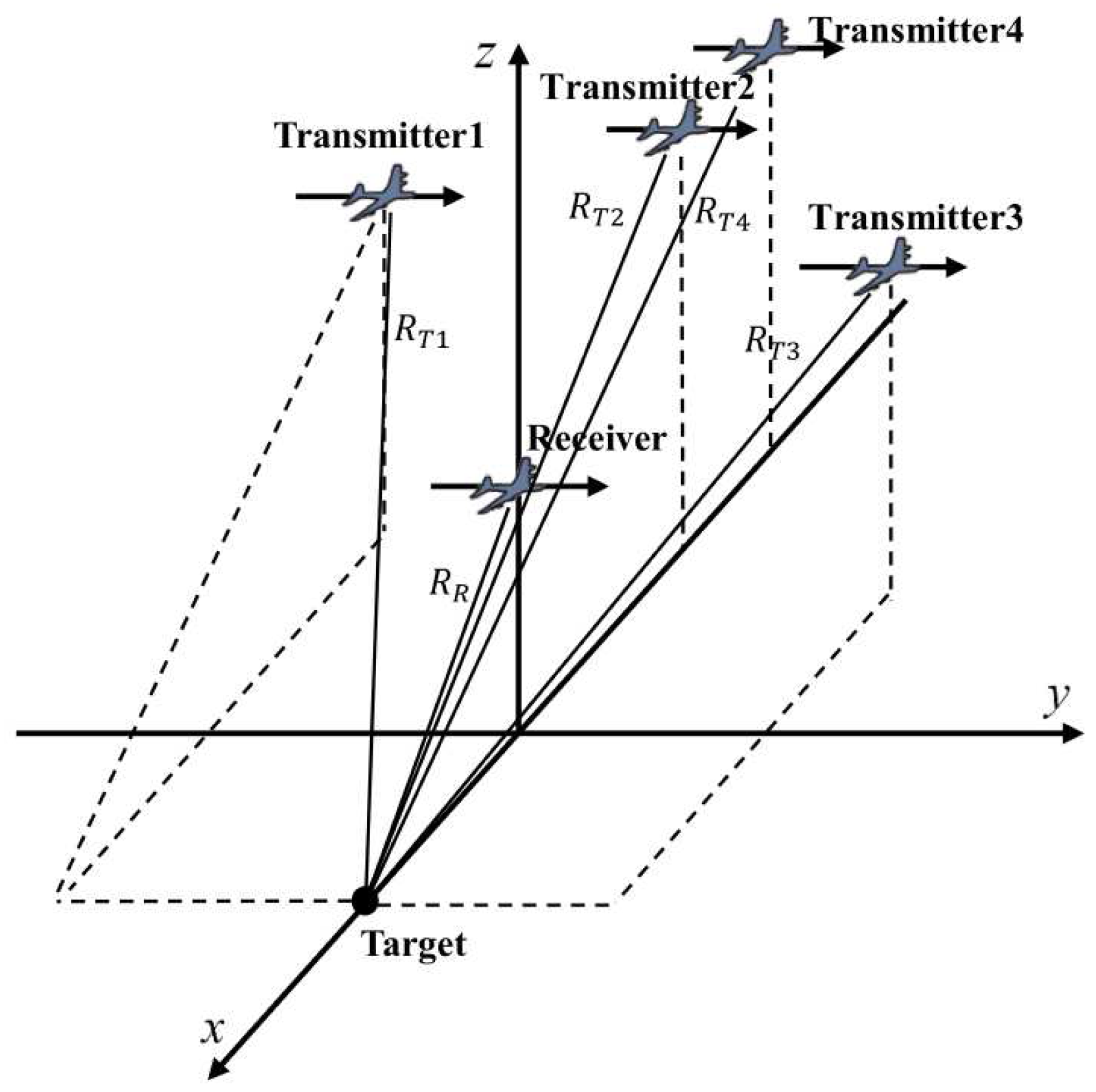
Multistatic synthetic aperture radar (SAR) has more than one transmitter and receiver, which makes it obtain more information of targets at different angles of view. Current studies on multistatic SAR mainly focus on imaging algorithm [1,2,3,4], synchronization [5], experiments [6] and target detection [7,8]. Target localization is of significant importance for both monostatic and multistatic SAR applications. It is necessary for ensuring the geometry calibration accuracy and effective understanding and interpretation of the radar images. Target localization plays a key role in target reconnoitering, map mapping and flood disaster evaluation. Therefore, it is significant to research the method and accuracy of localization. However, very limited research works are reported on this aspect for multistatic SAR. In addition, different from monostatic SAR, multistatic SAR can obtain more target information. Therefore, it makes the three-dimensional localization possible. To obtain the location information, generally we need to know the bistatic range sum (BRS). Nevertheless, multistatic SAR has more complicated geometrical relationships, as the transmitters and receivers are independent of each other. The double hyperbolic range histories lead to double square roots in the range equation of every transmitter and receiver (T/R) pair in multistatic SAR. Therefore, we can see that the localization of multistatic SAR, compared with monostatic SAR, is much more complicated.
For geolocation of monostatic SAR, there are three different kinds of localization methods. They are positioning with stereo SAR images, the fundamental principles of interferometric SAR images for positioning and positioning with a single SAR image. Positioning with stereo SAR images is based on the SAR structure model. Additionally, the three-dimensional coordinates of the corresponding ground points are calculated by the coordinates of the same image points of two SAR images. However, the number and the spatial distribution of ground control points can influence the accuracy of target localization [9]. The fundamental principles of interferometric SAR images for positioning utilize the interferometric phase information to achieve the target localization [10]. However, the target height information that is obtained with interferometric SAR has large error in areas with dramatic altitude changes, such as mountain terrain. Positioning with a single SAR image is based on the range-Doppler (RD) model for spaceborne monostatic SAR [11,12]. Additionally, target coordinates can be obtained by solving the range equation and Doppler equation. However, this method cannot obtain target height information.
When it comes to the localization problem of multistatic SAR, the three-dimensional localization is a significant advantage of multistatic SAR, but has not received enough attention. In [13], a three-dimensional surface reconstruction method is proposed. It uses the information of BRSs and phases of the target in each T/R pair image to solve the height of the target. However, it only uses the first order approximation of the height estimation function’s Taylor expansion. When the height range becomes larger, its accuracy cannot satisfy the request of localization. The localization problem in multistatic SAR is similar to localization in the ground-based multistatic radar system. There are some localization methods for multistatic radar systems. In [14], a localization method based on Taylor-series estimation is proposed. However, it cannot capture a close enough starting point and has large computational burden. Therefore, this method cannot be applied to multistatic SAR.
In addition, the accuracy of BRS estimation greatly influences the localization accuracy. The influence factor of BRS estimation error can be classified into two parts: (1) time of arrival (TOA) estimation error; (2) time synchronization error. In traditional multistatic radar systems, TOA estimation is a considerable challenge especially when the signal-to-noise ratio (SNR) is low. The multistatic SAR has a similar problem, which may affect the BRS estimation accuracy. In [15,16], TOA estimation algorithms are proposed to improve the estimation accuracy. As another main influence factor, time synchronization is also a big challenge for the application of the multistatic radar system, as well as multistatic SAR. Without time synchronization, BRS cannot be estimated accurately. The work in [5] proposes time synchronization technology for distributed SAR, including bistatic and multistatic SAR. In [17], a mathematical model considering the time synchronization error is given. Both [5,17] can observably reduce the time synchronization error between transmitters and receivers. Therefore, according to [5,17], the BRS estimation error in multistatic SAR is less than 5 m, because the maximum of time synchronization error is 15 ns.
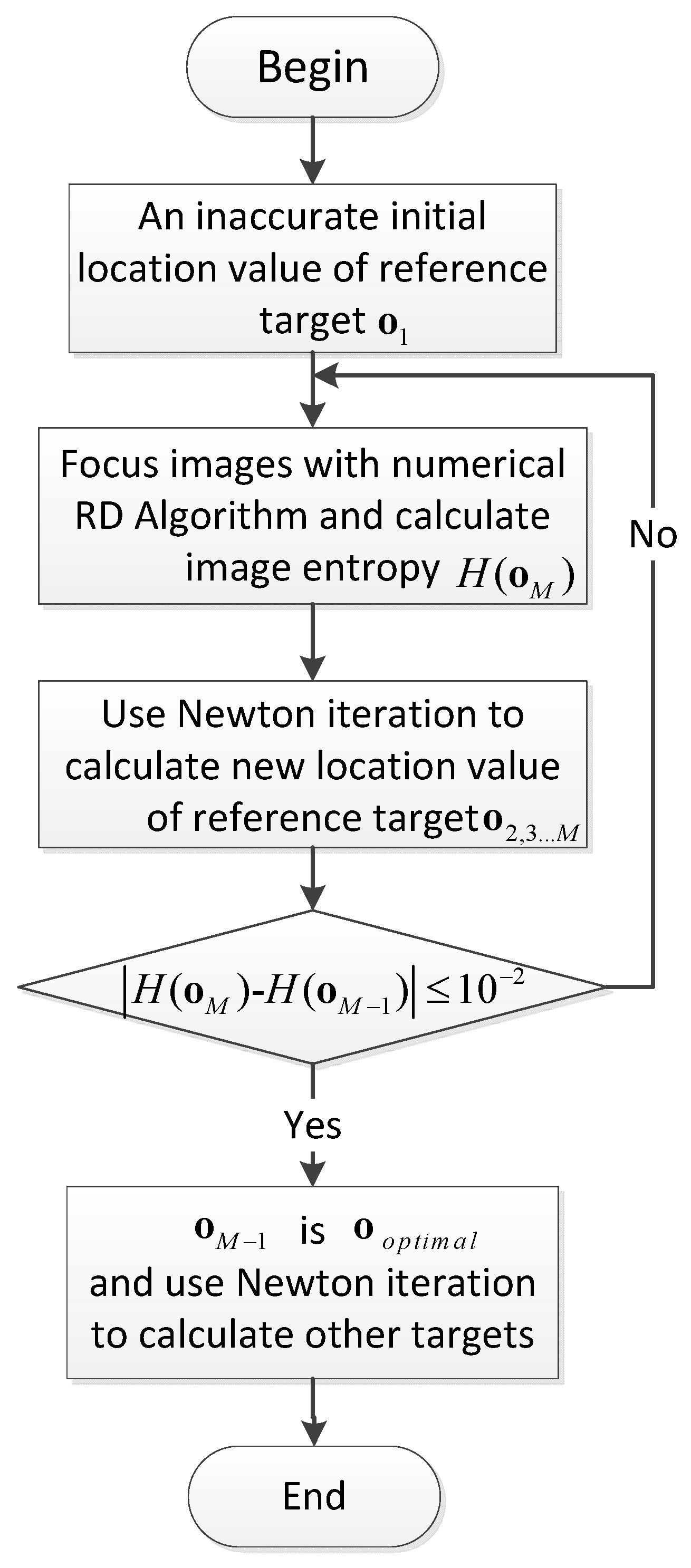
This paper describes a localization method for multistatic SAR. It can eliminate the influences of Doppler centroid estimation (DCE) errors and improve the localization accuracy. This method can be arranged into four steps: (1) the raw data from each T/R pair are focused by the numerical RD algorithm with the initial location value of the reference target; (2) Newton iteration is used to solve the target location value with the information of BRS in different SAR images with respect to different T/R pairs; (3) entropy is used to measure image quality and iterate imaging with the new location value of the reference target, until the entropy gets the minimum value; we can get the optimal location value of reference target; (4) all targets can be located by the Newton iteration method with their BRS in each T/R pair, which are obtained from the images with minimum entropy.
The fundament of the localization principle is presented in Section 2. In Section 3, simulation results are shown. Additionally, a comparison with other methods is shown in Section 4. At last, the conclusion is shown in Section 5.

2. Three-Dimensional Localization Method

The position of a target is determined by the BRSs of each T/R pair. Different T/R pairs have different BRS characteristics. For a given range bin in each T/R pair, the BRS is an ellipse in the imaging plane. Theoretically, the position of a target is the intersection of all ellipses with respect to all T/R pairs. To determine the position of a target in bistatic SAR image, a geometry coordinate system must be established. Figure 1 illustrates the geometry coordinate system for showing the position relationship between transmitters, receivers and target. Multiple transmitters and one receiver fly along the y axis. To obtain different SAR images with respect to different transmitters, the receiver should have multiple channels. In addition, the model and method in this paper can also be applied to the multistatic SAR configuration with multiple receivers and one transmitter.

2.1. Numerical RD Imaging Algorithm

As the only estimated parameter, BRS plays a significant role in localization. In multistatic SAR, BRS is obtained from the image result. Thus, the imaging accuracy of multistatic SAR is also an important factor in localization. In other words, if a target is focused on the wrong BRS cell, the accurate position of the target cannot be obtained. In order to obtain accurate BRS information, a precise bistatic SAR imaging algorithm is required. Due to the two square roots in range history, it is not easy to get the accurate analytical range cell migration (RCM) correction (RCMC) and the azimuth compression functions with respect to Doppler frequency in the bistatic SAR imaging process [18]. Here, an algorithm named numerical RD can solve these problems. It uses the numerical method to calculate the Doppler-domain RCMC functions. The RCM is computed directly for every sampled azimuth time. At the same time, there is an one-to-one relationship between the azimuth and Doppler frequency. Therefore, we can get the accurate relationship between RCM and Doppler frequency numerically. This algorithm effectively improves the RCMC performance [19]. In addition, through the numerical RD algorithm, we can get the accurate azimuth compression function with respect to the Doppler frequency.

2.1.1. SAR Path Interpolation

In the numerical RD algorithm, in order to obtain the accurate relationship between RCM and Doppler frequency, path interpolation should be performed firstly. The proposed method chooses spline interpolation as the interpolation method. Figure 2 shows the receiver path before and after spline interpolation, respectively.

2.1.2. Accurate Relationship between RCM and Doppler Frequency

In every azimuth time t, the BRS of reference target is:
R B ( t ; x , y , h ) = ( x x T ( t ) ) 2 + ( y y T ( t ) ) 2 + ( h h T ( t ) ) 2 + ( x x R ( t ) ) 2 + ( y y R ( t ) ) 2 + ( h h R ( t ) ) 2
where ( x , y , h ) , x T ( t ) , y T ( t ) , h T ( t ) and x R ( t ) , y R ( t ) , h R ( t ) are the locations of the target, transmitter and receiver, respectively. The position relationship between receiver, transmitter and target point in every azimuth moment is shown in Figure 3.
The Doppler frequency of the reference target at azimuth time t is:
f d c = V R · R R P λ R R P + V T · R T P λ R T P
where V R is the velocity vector of the receiver, V T is the velocity vector of the transmitter, R R P and R T P are the three-dimensional vectors from the receiver and transmitter to the reference target, respectively, and λ is the wavelength. The Doppler frequency and BRS are shown in Figure 4.
Therefore, through azimuth time, the one-to-one relationship between Doppler frequency and RCM is established, which is shown in Figure 5. Because we use the target location value in (1) and (2), theoretically, this relationship is not accurate before we finish the target localization. Here, we set an initial target location value to get an initial relationship between Doppler frequency and RCM.
At last, depending on the relationship between Doppler frequency and RCM, the RCMC is done to all range-compressed images with respect to the reference target from every T/R pair.

2.1.3. Azimuth Reference Signal Construction

The spatial variance of azimuth compression matched filter along the range direction is a traditional problem for bistatic or multistatic SAR. Additionally, the accurate azimuth compression function with respect to Doppler frequency cannot be obtained easily. Therefore, in order to guarantee the localization accuracy of the proposed method, it is significant to construct the azimuth reference signal of every range cell.
For instance, the position of a point is ( x i , y i ) (i means the index of the range cell). When the beam center crosses the point target, the positions of the receiver and transmitter in every T/R pair are ( x R , y R , h R ) and ( x T , y T , h T ) , respectively.
Then, if a point ( x j , y j ) has the same beam central moment as another point ( x i , y i ) , the following equations are obtained:
R B i Δ R = x j 2 + ( y j y R ) 2 + h R 2 + ( x j x T ) 2 + ( y j y T ) 2 + h T 2 y j y i = ( x j x i ) tan θ c
where R B i is the BRS of the range cell with index i, R B i Δ R is the BRS of the range cell with index j and θ c is determined by the slope of the line of targets in antenna phase centers (APCs) of one azimuth moment, as given in Figure 6.
The solution of (3) is:
x j = b 1 ± b 1 2 4 a 1 c 1 2 a 1 y j = ( x j x i ) tan θ c + y i
where x R = 0 ,
a 1 = 4 ( R B i Δ R ) 2 ( 1 + tan 2 θ c ) 4 [ x T + ( y T y R ) tan θ c ] 2 b 1 = 8 tan θ c ( R B i Δ R ) 2 [ ( y i x i tan θ c ) y R ] + 4 [ C 0 2 ( y T y R ) ( y i x i tan θ c ) ] [ x T + ( y T y R ) tan θ c ] c 1 = 4 ( R B i Δ R ) 2 { [ ( y i x i tan θ c ) y R ] 2 + h R 2 } [ 2 ( y T y R ) ( y i x i tan θ c ) C 0 ] 2 C 0 = x T 2 + y T 2 + h T 2 y R 2 h R 2 ( R B i Δ R ) 2
Based on position information of the range cell with index j point, the azimuth reference signal of the range cell with index j can be constructed by:
S j ( t ) = A 0 w a ( t ) exp j π K a j t + f d c j K a j 2
where A 0 is a constant parameter, w a ( t ) is the window function of azimuth,
f d c j = V R · R R P j λ R R P j + V R · R T P j λ R T P j
K a j = V T 2 cos 2 θ T s q c j λ R T P j + V R 2 cos 2 θ R s q c j λ R R P j
θ T s q c j = sin 1 V T · R T P j λ R T P j
θ R s q c j = sin 1 V R · R R P j λ R R P j
R R P j and R T P j are the three-dimensional vector from the receiver and transmitter to the point j.
Till now, we construct the RCMC function and azimuth compression function. Then, we can get the focused result.

2.2. Target Localization Method

Theoretically, using the BRS information of every range bin in images focused by the above numerical RD algorithm, we can get the location values with respect to every target by solving Equation (1). However, the BRS equation in (1) has double square roots. In addition, we have multiple BRS equations corresponding to different transmitters with respect to the same point target. It is not easy to get the precise and analytic solution. In the proposed method, the Newton iteration method is used to solve the localization problem of multistatic SAR. Additionally, the initial location value of the reference target in (1) and (2) is not accurate. Therefore, the RCMC and azimuth compression functions are not accurate actually. Then, the BRS estimation from the coarse focused image has large error. In order to get more accurate BRS, here, we use entropy to measure image quality and iterate imaging with new location value of reference target, until the entropy gets the minimum value. Therefore, we can get the optimal location value of the reference target, and the BRS estimation error will be reduced to the minimum.

2.2.1. Bistatic Range Sum Estimation

Firstly, the BRS should be estimated by using the time delay information:
R B i = c * t o f f s e t + i N r 2 1 f s
where c is the velocity of light, t o f f s e t is the time delay of the range bin of N r 2 + 1 , N r is the sample number in range, f s is the sample frequency and i is the index of the range bin.

2.2.2. Target BRS Equations

After estimating the BRSs in every T/R pair, the targets’ locations can be calculated by using (1). Each BRS means an ellipsoid surface, as given in Figure 7.
Technically, the position of the target is the intersection of those ellipses. Therefore, the target position is the unique solution for BRS equations. Using all of the information from every T/R pair, we can get BRS functions of a target as follows:
R B , 1 = ( x T 1 x ) 2 + ( y T 1 y ) 2 + ( h h T 1 ) 2 + ( x R x ) 2 + ( y R y ) 2 + ( h h R ) 2 R B , 2 = ( x T 2 x ) 2 + ( y T 2 y ) 2 + ( h h T 2 ) 2 + ( x R x ) 2 + ( y R y ) 2 + ( h h R ) 2 R B , N = ( x T N x ) 2 + ( y T N y ) 2 + ( h h T N ) 2 + ( x R x ) 2 + ( y R y ) 2 + ( h h R ) 2
Then, a calculation method is presented to solve these equations in the next subsection.

2.2.3. Newton Iteration Formula

The Newton iteration method is a way for nonlinear equation solutions. Based on Newton’s method and linear algebra, the iteration formula can be obtained as follows:
f B , 1 x x = x k f B , 1 y y = y k f B , 1 h h = h k f B , 2 x x = x k f B , 2 y y = y k f B , 2 h h = h k f B , N x x = x k f B , N y y = y k f B , N h h = h k x k + 1 y k + 1 h k + 1 = R B , 1 R B , 2 R B , N
where ( x k , y k , h k ) is the current position of the iteration point and ( x k + 1 , y k + 1 , h k + 1 ) is the next position of the iteration point. f B , N is the BRS equation in (1), and N corresponds to the N-th transmitter. • is matrix multiplication.
Therefore,
x k + 1 y k + 1 h k + 1 = f B , 1 x x = x k f B , 1 y y = y k f B , 1 h h = h k f B , 2 x x = x k f B , 2 y y = y k f B , 2 h h = h k f B , N x x = x k f B , N y y = y k f B , N h h = h k 1 R B , 1 R B , 2 R B , N
where 1 means the generalized inverse matrix.
The Newton iteration process of (13) is shown in Figure 8. In Figure 8, there are in total three iterations for solving the nonlinear Equation (12) from the start point to the end point. From Figure 8, we can see that the iteration point is closer and closer to the target position ( 1000 , 0 , 0 ) step by step using the proposed method. Finally, we can solve the nonlinear Equation (12) with accurate BRS in each T/R pair. Therefore, we can get the target position by solving the nonlinear Equation (12) with Newton iteration.

2.2.4. Entropy Minimization Principle

In Equation (1), the initial location value of the reference target is not accurate, which makes huge error. To ensure the accuracy, we use the entropy minimization principle [20] in this paper.
Let o = [ x , y , h ] T be the reference target location vector. Define the power normalized image as:
P i , j ( o ) = p i , j ( o ) 2 j = 1 J i = 1 I p i , j ( o ) 2
where i, j means the i-th range pixel and the j-th azimuth pixel in the SAR image, I(J) represents the number of pixels in the SAR image, in the range(azimuth) directions, and p is pixel value of SAR image.
The entropy function of the radar image is defined as:
H ( o ) = j = 1 J i = 1 I P i , j l n ( P i , j ( o ) )
The estimated location of the reference target is obtained by minimizing the entropy:
o o p t i m a l = arg min o { H ( o ) }
Till now, we can get the optimal location value of the reference target. Then, other targets’ location values can be obtained, as well, by Newton iteration in (13) with the BRS information of every target. Figure 9 gives the steps of three-dimensional localization method proposed in this paper. In Figure 9, M is the entropy minimization iteration times. Additionally, new location value of the reference target is calculated by the Newton iteration with new and more accurate BRS. When we get the accurate location value of the reference target that is also called the optimal location value of the reference target here, the radar image entropy is almost unchangeable in the subsequent iteration. Therefore, we can make sure that H ( o M 1 ) is minimum and o M 1 is the optimal location value of the reference target.

3. Numerical Simulation

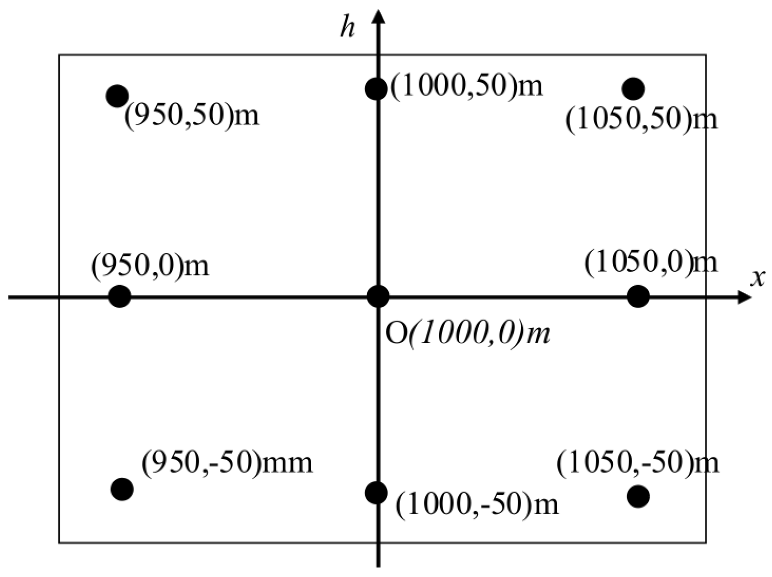
To verify the effectiveness of the proposed localization method based on the numerical RD algorithm and entropy minimization iteration, we carry out numerical simulations in this section. In the simulations, multistatic SAR is set to be one receiver and four transmitters. We set nine point targets, as shown in Figure 10. They distribute in one plane vertical to the ground with the same y axis value. This is to verify the capability of three-dimensional localization. The distances between two adjacent targets along the x axis direction and h axis direction are both 50 m. Target O is the center target. The simulation parameters are listed in Table 1.

3.1. Three-Dimensional Target Localization without Reference Target Location Error and Entropy Minimization Iteration

Firstly, we assume that the location of reference target O is already known precisely before we perform the imaging and localization. Thus, the reference target location has no error. Therefore, we do not need to perform entropy minimization iteration. At the same time, the transmitters’ and receiver’s locations are precise, as well. Based on the proposed method, the localization results are shown in Table 2. Additionally, the localization error is computed as the Euclidean distance between simulated and localized target points. We can find that the numerical RD imaging algorithm and Newton iteration are effective in the localization of multistatic SAR. The location errors of the other targets in Table 2 come from the estimation errors of BRS in the focused SAR image.

3.2. Three-Dimensional Target Localization with Reference Target Location Error and Entropy Minimization Iteration

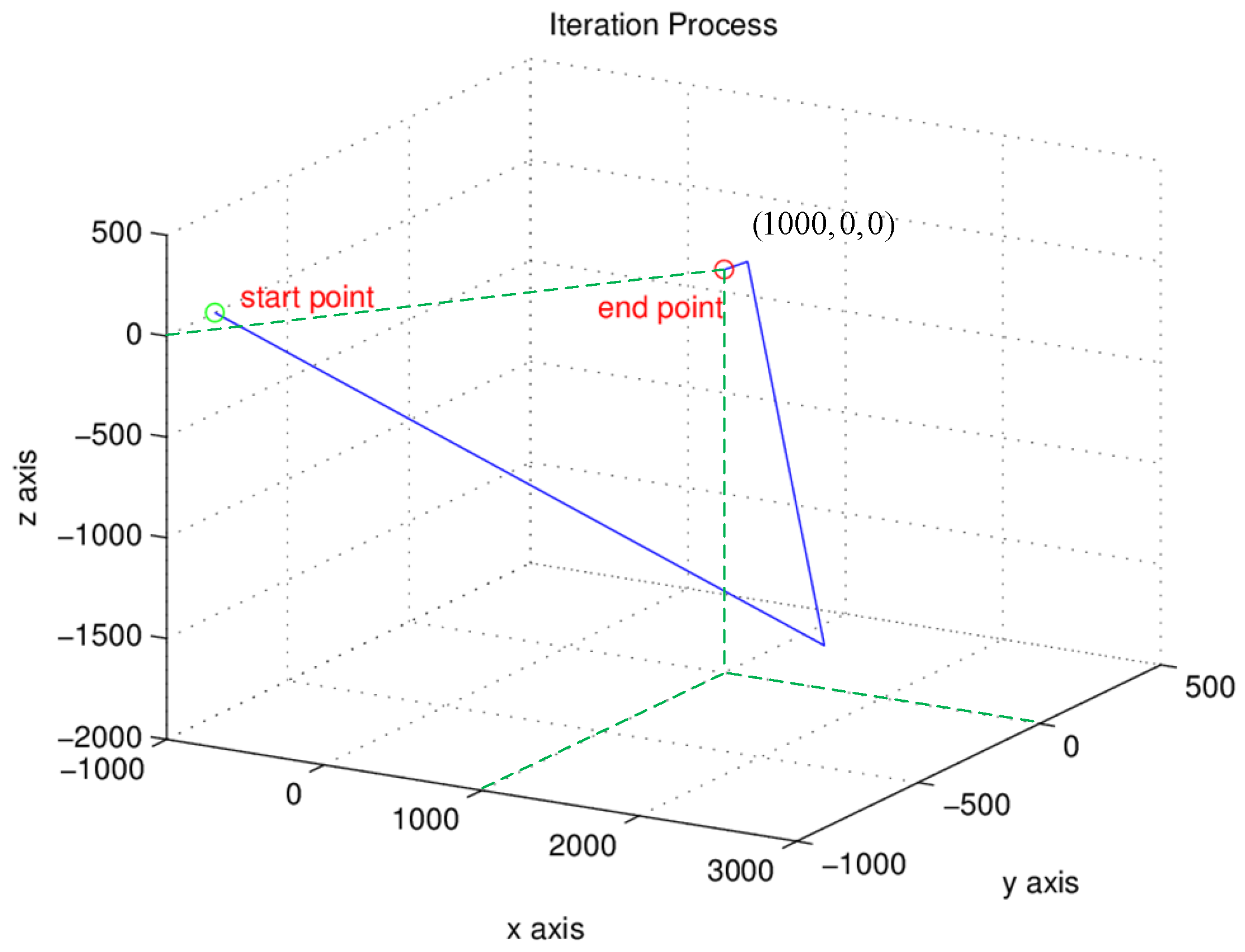
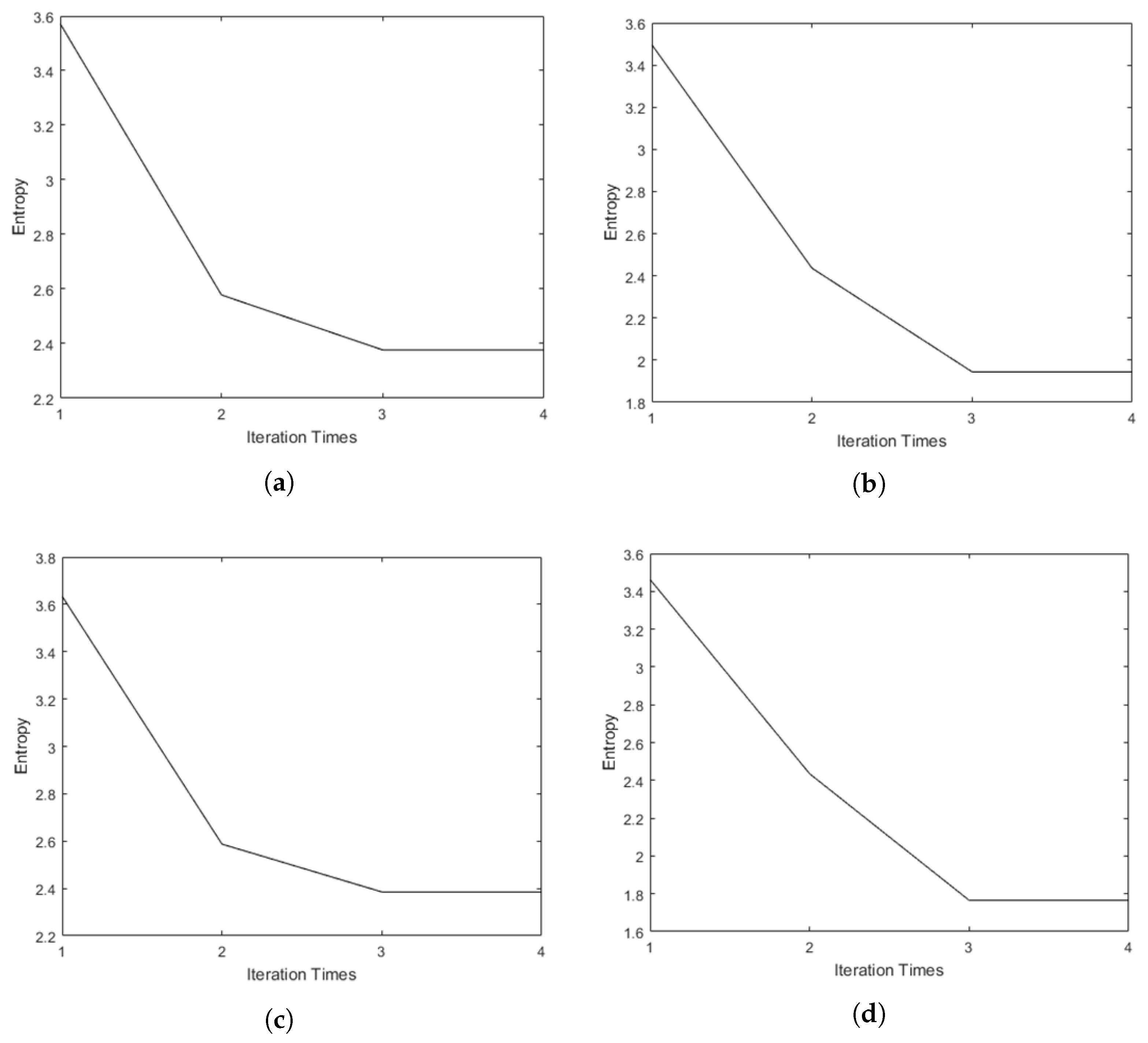
In this section, the location value of the reference target has a certain error. We use entropy minimization iteration to eliminate this error. The real position of the reference target is ( 1000 , 0 , 0 ) m, but the location value of the reference target that we can get is ( 984.1200 , 26.0809 , 0.0 ) m.
Then, we use entropy minimization iteration to improve the location value of the reference target. After three times of iteration, we can find that the entropy in each T/R pair reaches the minimum. The entropy minimization iteration process is shown in Figure 11.
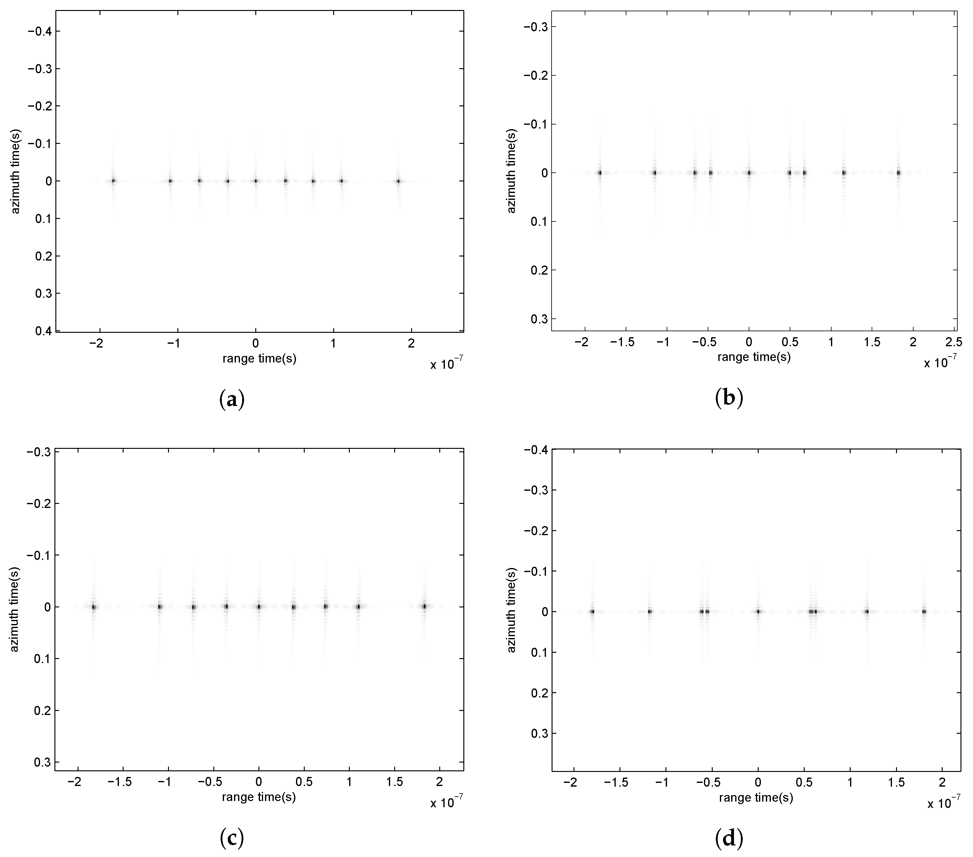
The raw data from every T/R pair are focused by the numerical RD algorithm with the reference target that is obtained from the three-time entropy minimization iteration. The focused images are shown in Figure 12.
Based on the three-dimensional localization method, the localization result is listed in Table 3.
Comparing with Table 2, we can see that the reference target location error does not influence the localization accuracy with this method.

3.3. Three-Dimensional Target Localization with the Platforms’ Position Error

From Equation (1), we know that the platforms’ position values have significant influences on the target localization of multistatic SAR. In addition, the platforms’ position values affect the imaging accuracy, as well. Here, we firstly assume that the error is small, where the position errors of the receiver, Transmitter 1, Transmitter 2, Transmitter 3 and Transmitter 4 are ( 0.7818 , 0.9186 , 0.0944 ) m, ( 0.3102 , 0.6748 , 0.7620 ) m, ( 0.033 , 0.9195 , 0.3192 ) m, ( 0.1705 , 0.5524 , 0.5025) m and ( 0.4898 , 0.0119 , 0.3982 ) m, respectively. The localization results are shown in Table 4.
When the platforms’ position has large error, the errors of the receiver, Transmitter 1, Transmitter 2, Transmitter 3 and Transmitter 4 are ( 4.1719 , 2.1416 , 2.5720 ) m, ( 3.1428 , 2.5648 , 4.2926 ) m, ( 1.5002 , 3.0340 , 2.4892 ) m, ( 1.1604 , 0.2671 , 1.4834 ) m and ( 3.3083 , 0.8526 , 0.4972 ) m, respectively. The localization results are shown in Table 5.
We can see that the platforms’ position error can influence the accuracy of target locations. Additionally, in Table 4, we can find that the maximal location error is less than 10 m, and the minimal location error is less than 5 m with this method. In Table 5, the location error is less than 17 m. Additionally, the three-dimensional localization method also can be applied to platforms’ with large error for some large targets like buildings and planes. Therefore, we can find that the localization error increases with the increase in the platforms’ position error.

3.4. Three-Dimensional Target Localization with the Platforms’ Velocity Error

The velocity error of the platforms is also important information for the proposed method, which can cause BRS estimation error.
The velocity errors of the receiver, Transmitter 1, Transmitter 2, Transmitter 3 and Transmitter 4 are 0.8213 m/s, −0.2004 m/s, −0.4803 m/s, 0.6001 m/s and −0.1372 m/s. The localization results are shown in Table 6. Additionally, we can see that the location position of the reference target has no error, and the maximal location error is less than 3.5 m with this method.

4. Discussion and Comparison

As a contrast, the localization result proposed in [11,12] with the same parameters in Table 1 is listed in Table 7. Since it is monostatic SAR, the location and velocity of the first transmitter parameter are used here. Additionally, in Table 8, we set the same targets without height information in our proposed method. We can find that the two methods can be applied to targets without height information, and localization error is less with the three-dimensional localization method. In addition, we set targets with height information, which is shown in Figure 10. The localization result proposed in [11,12] is shown in Table 9. It is clear in Table 9 that localization error is too large, and this method cannot be applied to obtain the target height information.
According to Table 2, Table 3, Table 4, Table 5 and Table 6, it can be concluded that the proposed localization method has a higher quality of accuracy and can obtain targets’ height information compared with that proposed in [11,12].

5. Conclusions

A localization method for multistatic SAR is proposed in this paper. It is based on the numerical RD algorithm and entropy minimization iteration. Numerical RD processing is used to focus the raw data of different transmitter and receiver pairs in multistatic SAR. However, in the focusing, the location value of the reference target is preset before we finish the target localization. Then, Newton iteration is used to obtain the three-dimensional coarse location values of the reference target. After that, to improve the localization accuracy, image entropy minimization iteration is carried out. In every iteration, the location values are updated until the image entropy obtains the minimum, which means the image is focused very well and the location value is precise. Finally, other targets’ location values are obtained from the BRS information. Therefore, the proposed algorithm can improve the localization accuracy and achieve three-dimensional localization.

Acknowledgments

This work is supported by the National Natural Science Foundation of China (No. 61401078), the National Natural Science Foundation of China (No. 61301273), the Research Fund for High-technology Project (No. 9140A07020614DZ02099) and the Research Startup Fund of the University of Electronic Science and Technology of China (No. Y02002010201089).

Author Contributions

Junjie Wu and Yushi Xu carried out all of the analyses and algorithms. Xuqi Zhong provided some of the plots shown in the manuscript. And Zhichao Sun and Jianyu Yang offered a lot of advice on the language.

Conflicts of Interest

The authors declare no conflict of interest.

References

  1. Zeng, H.C.; Wang, P.B.; Chen, J.; Liu, W.; Ge, L.; Yang, W. A Novel General Imaging Formation Algorithm for GNSS-Based Bistatic SAR. Sensors 2016, 16, 294. [Google Scholar] [CrossRef] [PubMed]
  2. Wu, J.; Li, Z.; Huang, Y.; Yang, J.; Yang, H.; Liu, Q.H. Focusing Bistatic Forward-Looking SAR with Stationary Transmitter Based on Keystone Transform and Nonlinear Chirp Scaling. IEEE Geosci. Remote Sens. Lett. 2014, 11, 148–152. [Google Scholar] [CrossRef]
  3. Wu, J.; Sun, Z.; Li, Z.; Huang, Y.; Yang, J.; Liu, Z. Focusing Translational Variant Bistatic Forward-Looking SAR Using Keystone Transform and Extended Nonlinear Chirp Scaling. Remote Sens. 2016, 8, 840. [Google Scholar] [CrossRef]
  4. Pu, W.; Li, W.; Wu, J.; Huang, Y.; Yang, J.; Yang, H. An Azimuth-Variant Autofocus Scheme of Bistatic Forward-Looking Synthetic Aperture Radar. IEEE Geosci. Remote Sens. Lett. 2017, 14, 1–5. [Google Scholar]
  5. Wang, W.Q. GPS-Based Time Phase Synchronization Processing for Distributed SAR. IEEE Trans. Aerosp. Electron. Syst. 2009, 45, 1040–1051. [Google Scholar] [CrossRef]
  6. Antoniou, M.; Zeng, Z.; Feifeng, L.; Cherniakov, M. Experimental Demonstration of Passive BSAR Imaging Using Navigation Satellites and a Fixed Receiver. IEEE Geosci. Remote Sens. Lett. 2012, 9, 477–481. [Google Scholar] [CrossRef]
  7. Wang, C.; Liao, M.; Li, X. Ship Detection in SAR Image Based on the Alpha-stable Distribution. Sensors 2008, 8, 4948. [Google Scholar] [CrossRef] [PubMed]
  8. Krishnapuram, B.; Sichina, J.; Carin, L. Physics-based detection of targets in SAR imagery using support vector machines. IEEE Sens. J. 2003, 3, 147–157. [Google Scholar] [CrossRef]
  9. Sansosti, E. A simple and exact solution for the interferometric and stereo SAR geolocation problem. IEEE Trans. Geosci. Remote Sens. 2004, 42, 1625–1634. [Google Scholar] [CrossRef]
  10. Lombardini, F.; Montanari, M.; Gini, F. Reflectivity estimation for multibaseline interferometric radar imaging of layover extended sources. IEEE Trans. Signal Process. 2003, 51, 1508–1519. [Google Scholar] [CrossRef]
  11. Curlander, J. Location of Spaceborne Sar Imagery. IEEE Trans. Geosci. Remote Sens. 1982, GE-20, 359–364. [Google Scholar] [CrossRef]
  12. Curlander, J.C. Utilization of Spaceborne SAR Data for Mapping. IEEE Trans. Geosci. Remote Sens. 1984, GE-22, 106–112. [Google Scholar] [CrossRef]
  13. Rigling, B.; Moses, R. Three-dimensional surface reconstruction from multistatic SAR images. IEEE Trans. Image Process. 2005, 14, 1159–1171. [Google Scholar] [CrossRef] [PubMed]
  14. Foy, W. Position-Location Solutions by Taylor-Series Estimation. IEEE Trans. Aerosp. Electron. Syst. 1976, AES-12, 187–194. [Google Scholar] [CrossRef]
  15. Bialer, O.; Raphaeli, D.; Weiss, A. Efficient Time of Arrival Estimation Algorithm Achieving Maximum Likelihood Performance in Dense Multipath. IEEE Trans. Signal Process. 2012, 60, 1241–1252. [Google Scholar] [CrossRef]
  16. Jeon, N.R.; Lee, H.B.; Park, C.G.; Cho, S.Y.; Kim, S.C. Superresolution TOA Estimation With Computational Load Reduction. IEEE Trans. Veh. Technol. 2010, 59, 4139–4144. [Google Scholar] [CrossRef]
  17. Zhang, X.; Li, H.; Wang, J. The Analysis of Time Synchronization Error in Bistatic SAR System. In Proceedings of the IEEE International Geoscience and Remote Sensing Symposium, Seoul, Korea, 25–29 July 2005; pp. 4619–4622. [Google Scholar]
  18. Qiu, X.; Ding, C.; Hu, D. Bistatic SAR Data Processing Algorithms; Wiley & Sons: Hoboken, NJ, USA, 2013. [Google Scholar]
  19. Bamler, R.; Meyer, F.; Liebhart, W. Processing of Bistatic SAR Data From Quasi-Stationary Configurations. IEEE Trans. Geosci. Remote Sens. 2007, 45, 3350–3358. [Google Scholar] [CrossRef]
  20. Xi, L.; Liu, G.; Ni, J. Autofocusing of ISAR images based on entropy minimization. IEEE Trans. Aerosp. Electron. Syst. 1999, 35, 1240–1252. [Google Scholar] [CrossRef]
Figure 1. Geometry coordinate system for the position relationship between transmitters, receiver and target.
Remotesensing 09 00470 g001
Figure 2. Receiver path before and after spline interpolation.
Remotesensing 09 00470 g002
Figure 3. Position relationship between receiver, transmitter and target point in every azimuth moment.
Remotesensing 09 00470 g003
Figure 4. Relationship between Doppler frequency, bistatic range sum and azimuth time.
Remotesensing 09 00470 g004
Figure 5. Relationship between RCM and Doppler frequency.
Remotesensing 09 00470 g005
Figure 6. Azimuth reference signal construction. (a) Processing result after range compression and RCMC; (b) targets’ position diagram.
Remotesensing 09 00470 g006
Figure 7. Transmitters, receiver and bistatic SAR (BSAR) iso-range (ellipses).
Remotesensing 09 00470 g007
Figure 8. Start point (green point), end point (red point) and Newton iteration process (blue line).
Remotesensing 09 00470 g008
Figure 9. Flowchart of the three-dimensional localization method.
Remotesensing 09 00470 g009
Figure 10. Target area used in the simulation.
Remotesensing 09 00470 g010
Figure 11. Entropy minimization iteration process. (a) Using the entropy minimization principle of the first T/R pair; (b) using the entropy minimization principle of the second T/R pair; (c) using the entropy minimization principle of the third T/R pair; (d) using the entropy minimization principle of the fourth T/R pair.
Remotesensing 09 00470 g011
Figure 12. Focused images. (a) The focused image of the first T/R pair; (b) the focused image of the second T/R pair; (c) the focused image of the third T/R pair; (d) the focused image of the fourth T/R pair.
Remotesensing 09 00470 g012
Table 1. Simulation parameters.
ParameterValue
Original LocationLocation of Receiver(0, 0, 0.5) km
Location of First Transmitter(−6, 1, 6) km
Location of Second Transmitter(−8, 0, 6) km
Location of Third Transmitter(−6, −1, 6) km
Location of Fourth Transmitter(−10, 0, 6) km
VelocityVelocity of Receiver50 m/s
Velocity of First Transmitter50 m/s
Velocity of Second Transmitter50 m/s
Velocity of Third Transmitter50 m/s
Velocity of Fourth Transmitter50 m/s
Signal ParameterCenter frequency9.65 GHz
Range Bandwidth400 MHz
Chirp Sign Duration2 μ s
Pulse Repetition Frequency (PRF)500 Hz
Table 2. Localization results without reference target location error and entropy minimization iteration.
TargetReal CoordinatesLocalization ResultLocalization Error
1(950,0,−50) m(950.8508,0.0,−48.6726) m1.5767 m
2(1000,0,−50) m(1000.8,0.0,−48.8) m1.4422 m
3(1050,0,−50) m(1049.6,0.0,−50.8) m0.8944 m
4(950,0,0) m(951.2372,0.0,2.1389) m2.4709 m
5(1000,0,0) m(1000.0,0.0,0.0000) m0.0000 m
6(1050,0,0) m(1050.6,0.0,1.1) m1.2530 m
7(950,0,50) m(950.4404,0.0,50.6659) m0.7984 m
8(1000,0,50) m(999.2073,0.0,48.7860) m1.4499 m
9(1050,0,50) m(1049.6,0.0,49.3) m0.8062 m
Table 3. Imaging reference target localization error simulation results.
TargetReal CoordinatesLocalization ResultLocalization Error
1(950,0,−50) m(950.8508,0.0,−48.6726) m1.5767 m
2(1000,0,−50) m(1000.8,0.0,−48.8) m1.4422 m
3(1050,0,−50) m(1049.6,0.0,−50.8) m0.8944 m
4(950,0,0) m(951.2372,0.0,2.1389) m2.4709 m
5(1000,0,0) m(1000.0,0.0,0.0000) m0.0000 m
6(1050,0,0) m(1050.6,0.0,1.1) m1.2530 m
7(950,0,50) m(950.4404,0.0,50.6659) m0.7984 m
8(1000,0,50) m(999.2073,0.0,48.7860) m1.4499 m
9(1050,0,50) m(1049.6,0.0,49.3) m0.8062 m
Table 4. Platforms’ position with small error simulation results.
TargetReal CoordinatesLocalization ResultLocalization Error
1(950,0,−50) m(951.5682,5.7927,−46.9796) m6.7184 m
2(1000,0,−50) m(1001.5,5.8,−47.1) m6.6558 m
3(1050,0,−50) m(1050.3,5.8,−49.1) m5.8771 m
4(950,0,0) m(952.3859,5.7720,4.4584) m7.6737 m
5(1000,0,0) m(1001.9,2.9,3.8) m5.1439 m
6(1050,0,0) m(1051.3,5.8,2.8) m6.5704 m
7(950,0,50) m(951.7403,5.7515,53.8226) m7.1218 m
8(1000,0,50) m(1001.1,8.7,52.7) m9.1755 m
9(1050,0,50) m(1051.4,2.9,53.3) m4.6109 m
Table 5. Platforms’ position with large error simulation results.
TargetReal CoordinatesLocalization ResultLocalization Error
1(950,0,−50) m(944.8372,−14.4786,−54.7489) m16.0884 m
2(1000,0,−50) m(994.2477,−11.6298,−55.6799) m14.1634 m
3(1050,0,−50) m(1044.8,−14.6,−54.8) m16.2247 m
4(950,0,0) m(943.9405,−14.4282,−6.1868) m16.8276 m
5(1000,0,0) m(995.7649,−14.4863,−3.3895) m15.4686 m
6(1050,0,0) m(1045.1,−11.6,−4.5) m13.3724 m
7(950,0,50) m(944.8908,−14.3770,45.1112) m16.0219 m
8(1000,0,50) m(995.0474,−14.4363,45.3140) m15.9654 m
9(1050,0,50) m(1044.1,−14.5,43.6) m16.9121 m
Table 6. Velocity error simulation results.
TargetReal CoordinatesLocalization ResultLocalization Error
1(950,0,−50) m(950.7647,−2.8967,−50.6680) m3.0695 m
2(1000,0,−50) m(1001.3,0.0000,−49.2) m1.5264 m
3(1050,0,−50) m(1049.8,0.0000,−51.0) m1.0198 m
4(950,0,0) m(950.6784,−2.8864,0.4979) m3.0066 m
5(1000,0,0) m(1000.0,0.0,0.0) m0.0000 m
6(1050,0,0) m(1049.9,−0.0000,0.6) m0.6083 m
7(950,0,50) m(948.8192,0.0000,48.6952) m1.7598 m
8(1000,0,50) m(998.6976,0.0000,49.1638) m1.5477 m
9(1050,0,50) m(1049.6,−2.9,51.4) m3.2450 m
Table 7. Targets localization result proposed in [11,12] without height information.
TargetReal CoordinatesLocalization ResultLocalization Error
1(950,−50,0) m(935.8925,−75.3489,0) m29.0101 m
2(1000,−50,0) m(983.0307,−76.1543,0) m31.1770 m
3(1050,−50,0) m(1033.1435,−75.5412,0) m30.6012 m
4(950,0,0) m(935.4895,−26.1256,0) m29.8848 m
5(1000,0,0) m(984.1200,−26.0809,0) m30.5350 m
6(1050,0,0) m(1033.0598,−25.8954,0) m30.9442 m
7(950,50,0) m(936.5635,24.0257,0) m29.2439 m
8(1000,50,0) m(985.8314,24.0645,0) m29.5533 m
9(1050,50,0) m(1033.4633,26.8441,0) m28.4545 m
Table 8. Localization result with the three-dimensional method.
TargetReal CoordinatesLocalization ResultLocalization Error
1(950,−50,0) m(951.7959,−50.0,1.0358) m2.0732 m
2(1000,−50,0) m(999.9852,−50.7312,0.0023) m0.7314 m
3(1050,−50,0) m(1050.3420,−50.0,0.8253) m0.8934 m
4(950,0,0) m(951.4626,0.0,2.1348) m2.5878 m
5(1000,0,0) m(1000.0,0.0,0.0) m0.0000 m
6(1050,0,0) m(1050.6820,0.0,1.1935) m1.3746 m
7(950,50,0) m(951.7965,50.0,1.1357) m2.1254 m
8(1000,50,0) m(999.9704.51.0014,−0.0483) m1.0030 m
9(1050,50,0) m(1050.7732,50.0004,1.4403) m1.6347 m
Table 9. Targets localization result proposed in [11,12] with height information.
TargetReal CoordinatesLocalization ResultLocalization Error
1(950,0,−50) m(992.7662,−2.8964,0.0) m65.8585 m
2(1000,0,−50) m(1042.4907,−2.9081,0.0) m65.6804 m
3(1050,0,−50) m(1092.1895,−2.9199,0.0) m65.4865 m
4(950,0,0) m(935.4895,−26.1256,0) m29.8848 m
5(1000,0,0) m(984.1200,−26.0809,0) m30.5350 m
6(1050,0,0) m(1033.0598,−25.8954,0) m30.9442 m
7(950,0,50) m(906.4636,−2.8761,0.0) m66.3603 m
8(1000,0,50) m(956.7748,−2.8879,0.0) m66.1571 m
9(1050,0,50) m(1007.0816,−2.8998,0.0) m65.9576 m

