
Automatic Sky View Factor Estimation from Street View Photographs—A Big Data Approach

 ,
,
Abstract
:1. Introduction
2. Methods
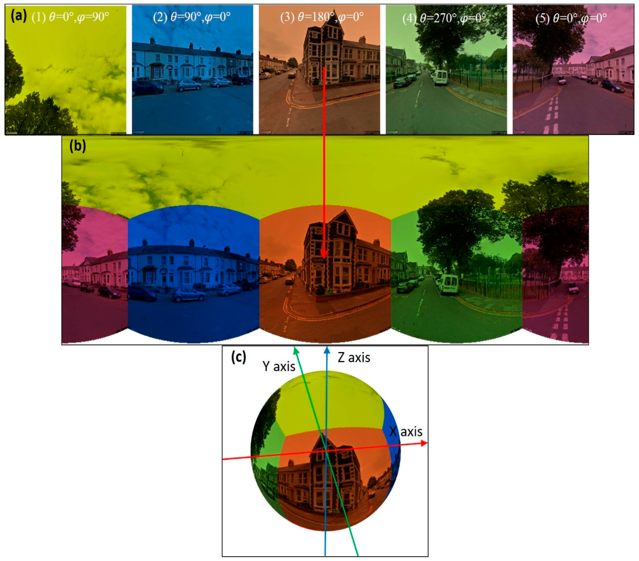
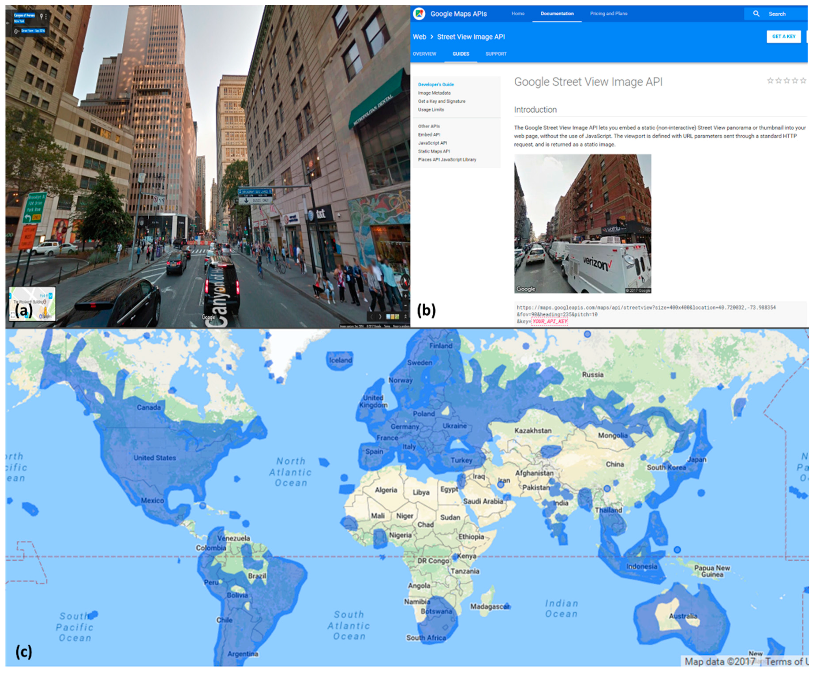
2.1. Retrieval and Stitching of Street View Images
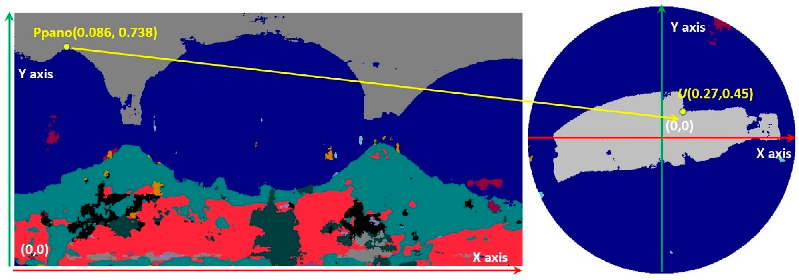
- Transform the normalized image coordinates Ppano(u, v) (Ppanou ∈ [0, 1], Ppanov ∈ [0, 1]) into spherical coordinates Pspherical(lon, lat). This can be easily done with the row/column index and the spherical extent associated with the panoramic image.
- Transform the spherical coordinates Pspherical(lon, lat) into world space coordinates Pworld(x, y, z).
- Loop over the set of images and transform the world space coordinates Pworld(x, y, z, 1.0) into clip-space coordinates Pclip(x, y, z, w) by multiplying Pworld(x, y, z, 1.0) by MatViewProj for each image. The following equation is used to transform Pworld(x, y, z, 1) into normalized screen space coordinates Pimage(u, v):where, Pimageu ∈ [0, 1], Pimagev ∈ [0, 1]. If Pimageu ∉ [0, 1] or Pimagev ∉ [0, 1], the image being considered is disregarded. Otherwise, a color value is sampled from this image at Pimage(u, v) and copied to Ppano(u, v).
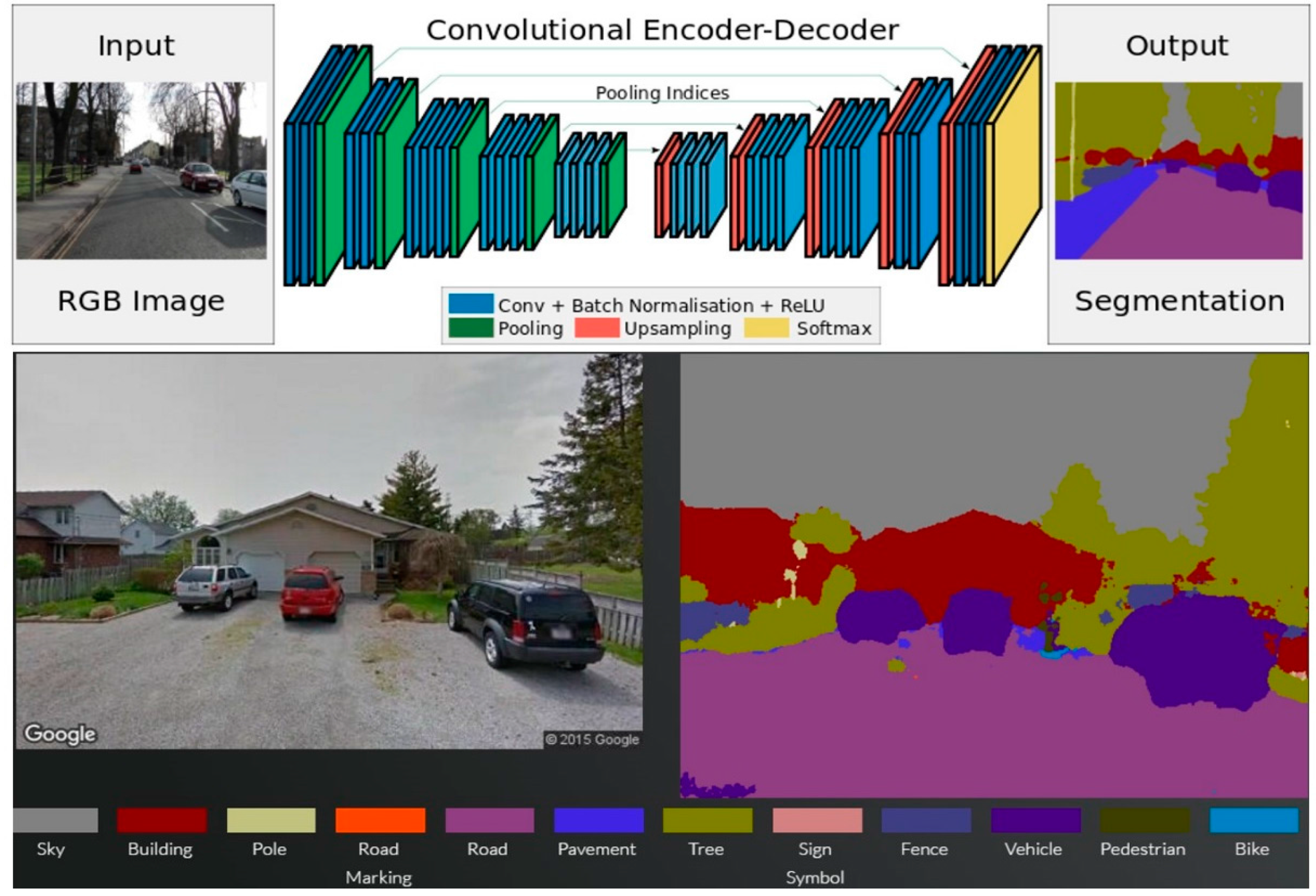
2.2. A Deep Learning Model for Classifying Street View Images
2.3. Hemispherical Transformation and Calculation of SVF
3. Comparisons and Application
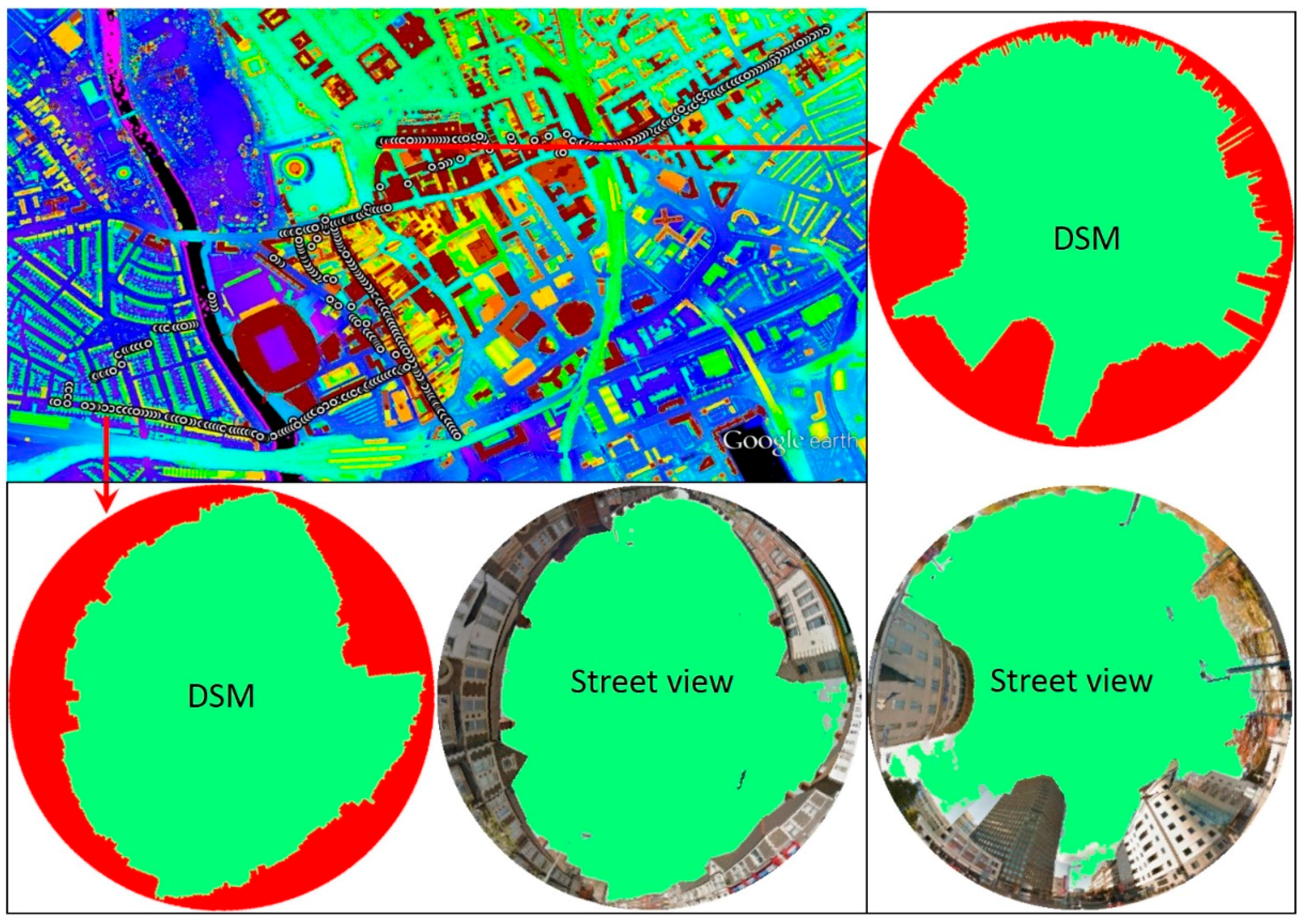
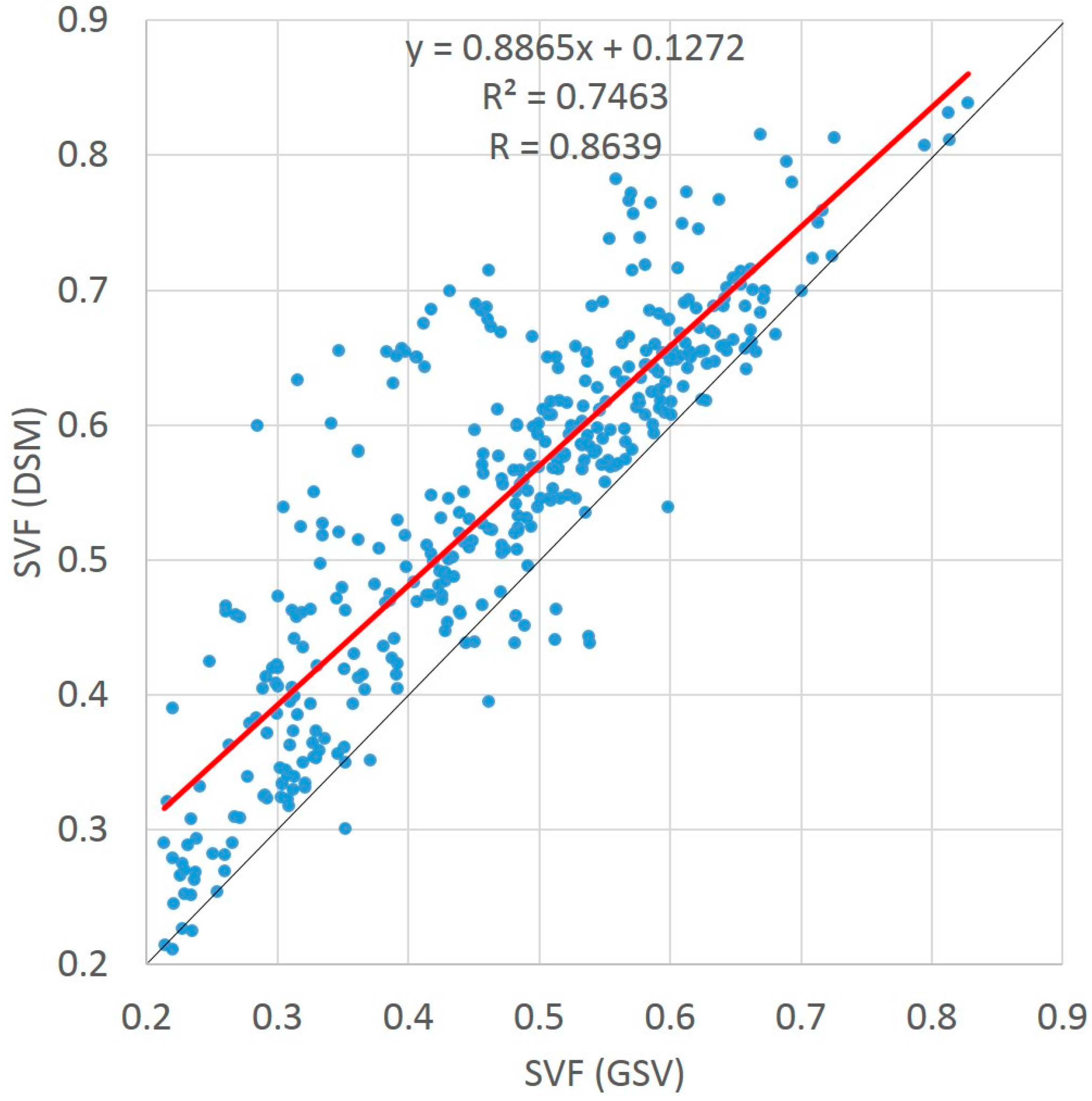
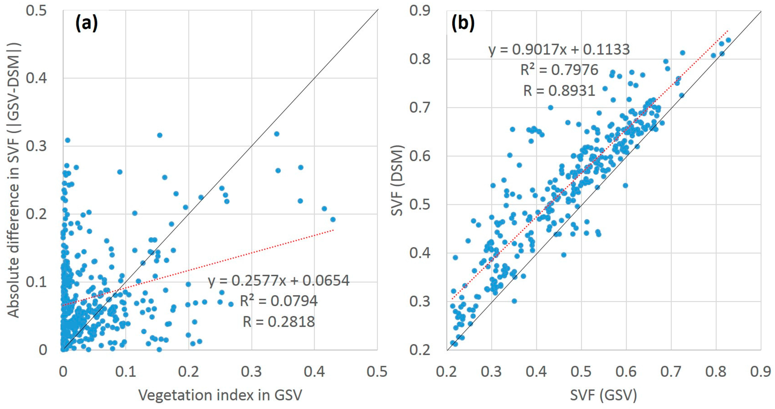
3.1. Comparison with SVF Estimates from a LiDAR-Derived DSM
- Read the surface height at the location from the DSM.
- Set the observation height at 2.4 m above the surface. We assume that the GSV vehicle has a height of 1.4 m and the camera is mounted 1 m above the vehicle.
- Calculate the horizon angle along each azimuthal direction in increments of 0.1 degree. This creates a hemispherical representation of the sky bounded by 3600 points, each of which is given by r and θ in the polar coordinate system, where r is the normalized horizon angle [0, 1] and θ is the normalized azimuthal angle [0, 1] respectively.
- Allocate a 1024-by-1024 image for rasterizing the sky boundary. In the rasterization, the horizon points are converted into image coordinates and the area within the sky boundary is filled with a color different than the non-sky area. The SVF is estimated using the same method as described in Section 2.3.
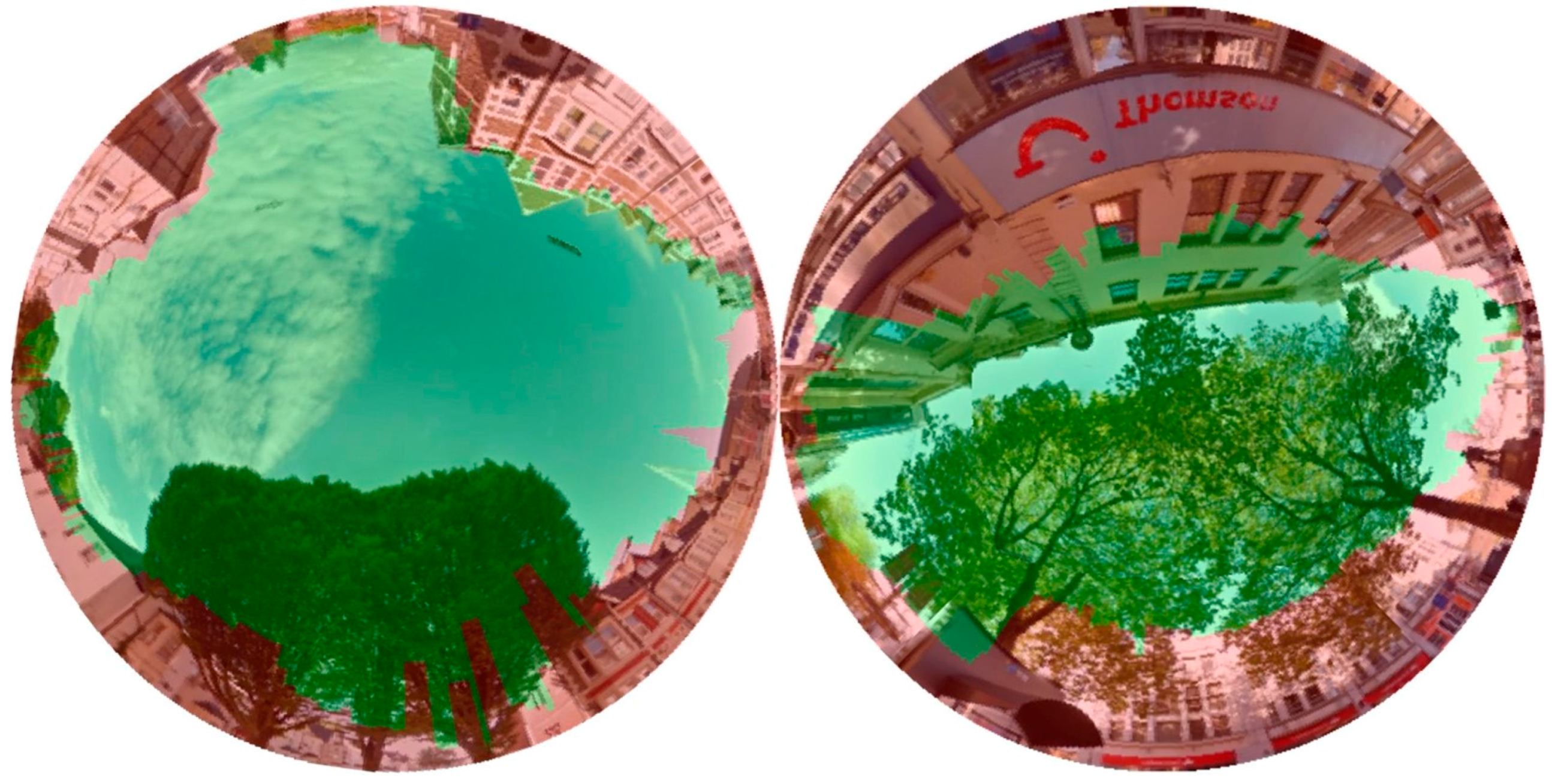
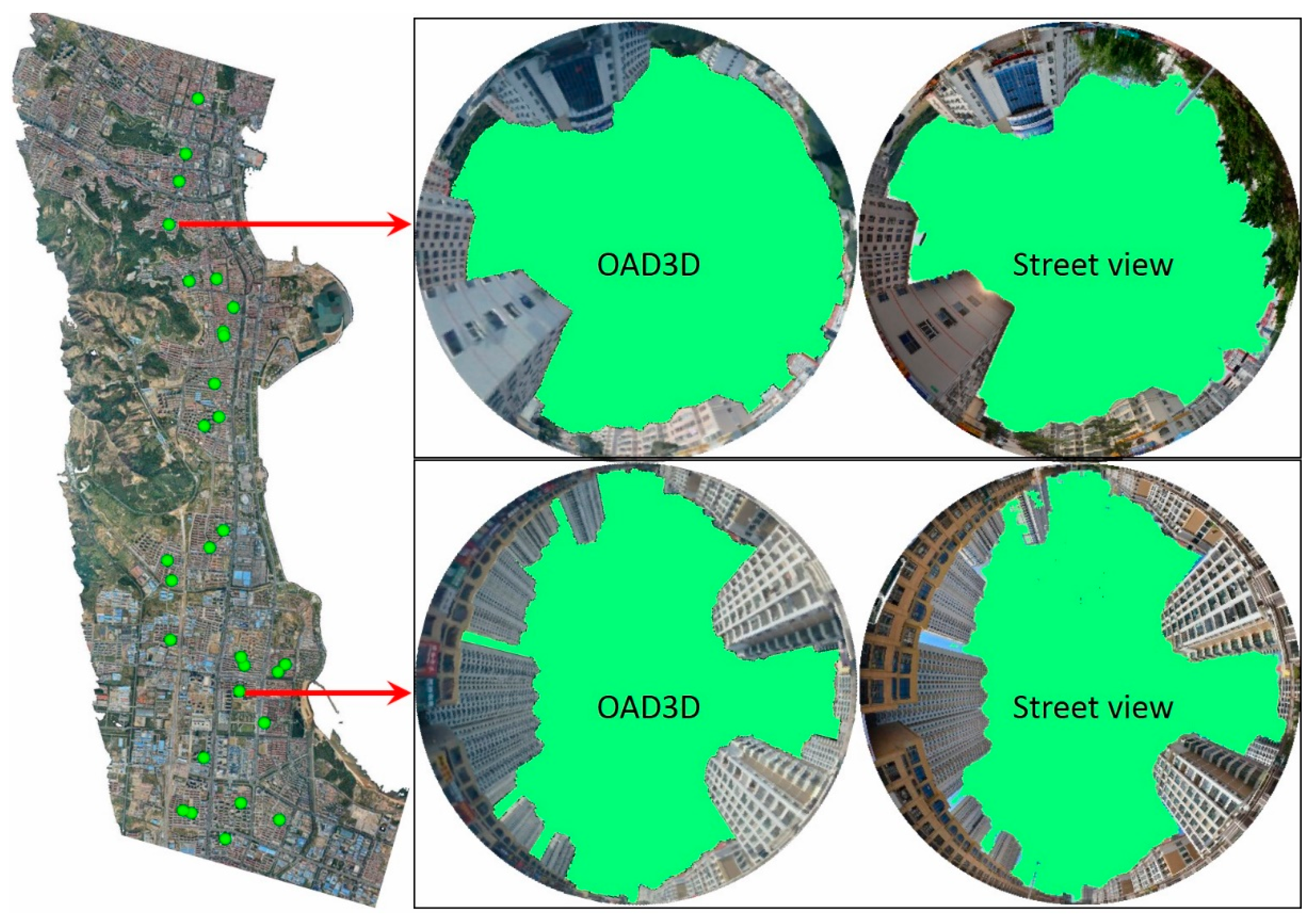
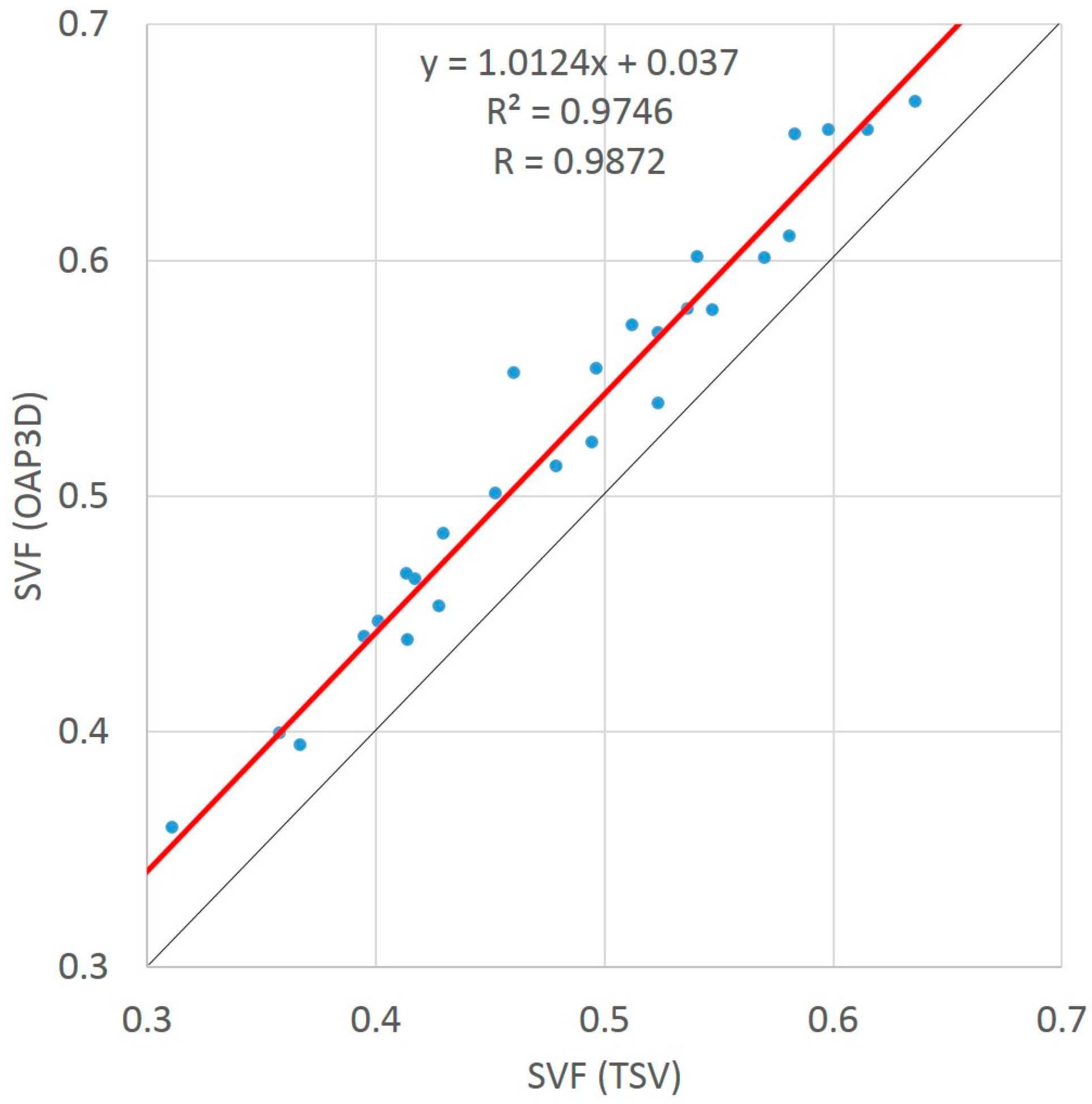
3.2. Comparison with SVF Estimates from a High-Resolution OAP3D
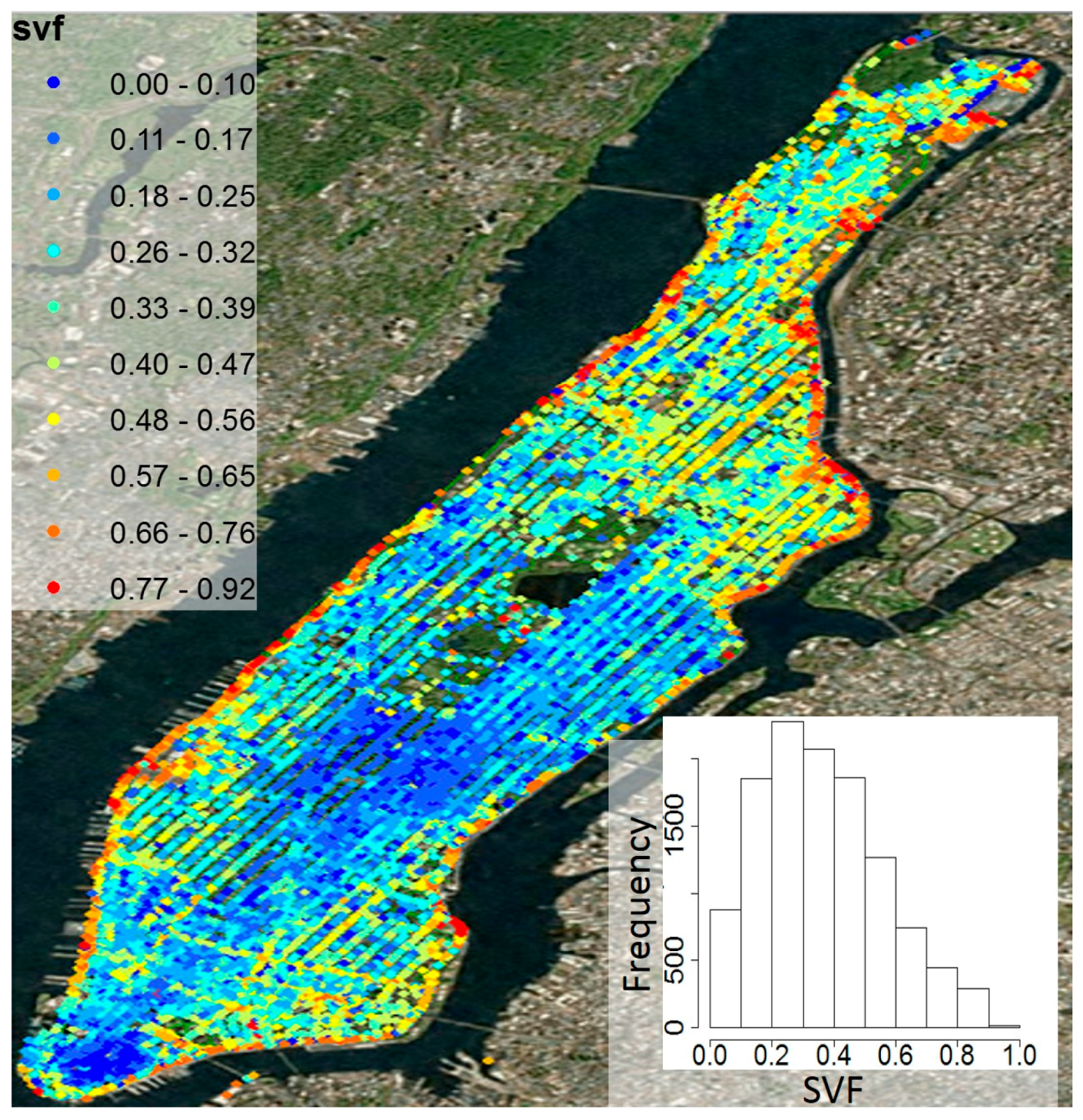
3.3. Application in Manhattan
4. Discussion
5. Conclusions
Acknowledgments
Author Contributions
Conflicts of Interest
References
- Oke, T.R. Canyon geometry and the nocturnal urban heat island: Comparison of scale model and field observations. Int. J. Climatol. 1981, 1, 237–254. [Google Scholar] [CrossRef]
- Gal, T.; Lindberg, F.; Unger, J. Computing continuous sky view factors using 3D urban raster and vector databases: Comparison and application to urban climate. Theor. Appl. Climatol. 2009, 95, 111–123. [Google Scholar] [CrossRef]
- Lindberg, F. Modelling the urban climate using a local governmental geo-database. Meteorol. Appl. 2007, 14, 263–274. [Google Scholar] [CrossRef]
- Krüger, E.L.; Minella, F.O.; Rasia, F. Impact of urban geometry on outdoor thermal comfort and air quality from field measurements in Curitiba, Brazil. Build. Environ. 2011, 46, 621–634. [Google Scholar] [CrossRef]
- Johansson, E. Influence of urban geometry on outdoor thermal comfort in a hot dry climate: A study in Fez, Morocco. Build. Environ. 2006, 41, 1326–1338. [Google Scholar] [CrossRef]
- Eliasson, I. The use of climate knowledge in urban planning. Landsc. Urban Plan. 2000, 48, 31–44. [Google Scholar] [CrossRef]
- Wei, R.; Song, D.; Wong, N.H.; Martin, M. Impact of Urban Morphology Parameters on Microclimate. Procedia Eng. 2016, 169, 142–149. [Google Scholar] [CrossRef]
- Bourbia, F.; Boucheriba, F. Impact of street design on urban microclimate for semi-arid climate (Constantine). Renew. Energy 2010, 35, 343–347. [Google Scholar] [CrossRef]
- Unger, J. Intra-urban relationship between surface geometry and urban heat island: Review and new approach. Clim. Res. 2004, 27, 253–264. [Google Scholar] [CrossRef]
- Nguyen, H.T.; Joshua, M.P. Incorporating shading losses in solar photovoltaic potential assessment at the municipal scale. Sol. Energy 2012, 86, 1245–1260. [Google Scholar] [CrossRef]
- Corripio, J.G. Vectorial algebra algorithms for calculating terrain parameters from DEMs and solar radiation modelling in mountainous terrain. Int. J. Geogr. Inf. Sci. 2003, 17, 1–23. [Google Scholar] [CrossRef]
- Li, X.; Zhang, S.; Chen, Y. Error assessment of grid-based diffuse solar radiation models. Int. J. Geogr. Inf. Sci. 2016, 30, 2032–2049. [Google Scholar] [CrossRef]
- Yang, J.; Wong, M.S.; Menenti, M.; Nichol, J. Modeling the effective emissivity of the urban canopy using sky view factor. ISPRS J. Photogramm. Remote Sens. 2015, 105, 211–219. [Google Scholar] [CrossRef]
- Yang, J.; Wong, M.S.; Menenti, M.; Nichol, J.; Voogt, J.; Krayenhoff, E.S.; Chan, P.W. Development of an improved urban emissivity model based on sky view factor for retrieving effective emissivity and surface temperature over urban areas. ISPRS J. Photogramm. Remote Sens. 2016, 122, 30–40. [Google Scholar] [CrossRef]
- Mandanici, E.; Conte, P.; Girelli, V.A. Integration of Aerial Thermal Imagery, LiDAR Data and Ground Surveys for Surface Temperature Mapping in Urban Environments. Remote Sens. 2016, 8, 880. [Google Scholar] [CrossRef]
- Zakšek, K.; Oštir, K.; Kokalj, Ž. Sky-View Factor as a Relief Visualization Technique. Remote Sens. 2011, 3, 398–415. [Google Scholar] [CrossRef]
- Souza, L.C.L.; Rodrigues, D.S.; Mendes, J.F.G. Sky-view factors estimation using a 3D-GIS extension. In Proceedings of the 8th International IBPSA Conference, Eindhoven, The Netherlands, 11–14 August 2003. [Google Scholar]
- Matzarakis, A.; Matuschek, O. Sky view factor as a parameter in applied climatology—Rapid estimation by the SkyHelios model. Meteorol. Z. 2011, 20, 39–45. [Google Scholar] [CrossRef]
- Hodul, M.; Knudby, A.; Ho, H.C. Estimation of Continuous Urban Sky View Factor from Landsat Data Using Shadow Detection. Remote Sens. 2016, 8, 568. [Google Scholar] [CrossRef]
- Holmer, B. A simple operative method for determination of sky view factors in complex urban canyons from fisheye photographs. Meteorol. Z. 1992, 236–239. [Google Scholar]
- Bradley, A.V.; Thornes, J.E.; Chapman, L. A method to assess the variation of urban canyon geometry from sky view factor transects. Atmos. Sci. Lett. 2001, 2, 155–165. [Google Scholar] [CrossRef]
- Moin, U.M.; Tsutsumi, J.I. Rapid estimation of sky view factor and its application to human environment. J. Hum. Environ. Syst. 2004, 7, 83–87. [Google Scholar] [CrossRef]
- Svensson, M.K. Sky view factor analysis–implications for urban air temperature differences. Meteorol. Appl. 2004, 11, 201–211. [Google Scholar] [CrossRef]
- Lindberg, F.; Grimmond, C.S.B. Continuous sky view factor maps from high resolution urban digital elevation models. Clim. Res. 2010, 42, 177–183. [Google Scholar] [CrossRef]
- McAfee, A.; Brynjolfsson, E.; Davenport, T.H.; Patil, D.J.; Barton, D. Big data: The management revolution. Harv. Bus. Rev. 2012, 90, 61–67. [Google Scholar]
- Al-Jarrah, O.Y.; Yoo, P.D.; Muhaidat, S.; Karagiannidis, G.K.; Taha, K. Efficient machine learning for big data: A review. Big Data Res. 2015, 2, 87–93. [Google Scholar] [CrossRef]
- Anguelov, D.; Dulong, C.; Filip, D.; Frueh, C.; Lafon, S.; Lyon, R.; Ogale, A.; Vincent, L.; Weaver, J. Google Street View: Capturing the world at street level. Computer 2010, 43, 32–38. [Google Scholar] [CrossRef]
- Google Street View (GSV). Available online: https://developers.google.com/maps/documentation/streetview/ (accessed on 10 February 2017).
- Baidu Street View (BSV). Available online: http://lbsyun.baidu.com/index.php?title=static (accessed on 10 February 2017).
- Tencent Street View (TSV). Available online: http://lbs.qq.com/panostatic_v1/ (accessed on 10 February 2017).
- Carrasco-Hernandez, R.; Smedley, A.R.D.; Webb, A.R. Using urban canyon geometries obtained from Google Street View for atmospheric studies: Potential applications in the calculation of street level total shortwave irradiances. Energy Build. 2015, 86, 340–348. [Google Scholar] [CrossRef]
- Yin, L.; Wang, Z. Measuring visual enclosure for street walkability: Using machine learning algorithms and Google Street View imagery. Appl. Geogr. 2016, 76, 147–153. [Google Scholar] [CrossRef]
- Yin, L.; Cheng, Q.; Wang, Z.; Shao, Z. ‘Big data’ for pedestrian volume: Exploring the use of Google Street View images for pedestrian counts. Appl. Geogr. 2015, 63, 337–345. [Google Scholar] [CrossRef]
- Li, X.; Zhang, C.; Li, W.; Ricard, R.; Meng, Q.; Zhang, W. Assessing street-level urban greenery using Google Street View and a modified green view index. Urban For. Urban Green. 2015, 14, 675–685. [Google Scholar] [CrossRef]
- Rundle, A.G.; Bader, M.D.; Richards, C.A.; Neckerman, K.M.; Teitler, J.O. Using Google Street View to audit neighborhood environments. Am. J. Prev. Med. 2011, 40, 94–100. [Google Scholar] [CrossRef] [PubMed]
- LeCun, Y.; Bengio, Y.; Hinton, G. Deep learning. Nature 2015, 521, 436–444. [Google Scholar] [CrossRef] [PubMed]
- Shirley, P.; Ashikhmin, M.; Marschner, S. Fundamentals of Computer Graphics; CRC Press: Boca Raton, FL, USA, 2009. [Google Scholar]
- Krizhevsky, A.; Hinton, G.E.; Sutskever, I. ImageNet Classification with Deep Convolutional Neural Networks. In Proceedings of the 25th International Conference on Neural Information Processing Systems, Lake Tahoe, NV, USA, 3–6 December 2012. [Google Scholar]
- Seide, F.; Li, G.; Chen, X.; Yu, D. Feature engineering in Context-Dependent Deep Neural Networks for conversational speech transcription. In Proceedings of the 2011 IEEE Workshop on Automatic Speech Recognition and Understanding (ASRU), Waikoloa, HI, USA, 11–15 December 2011. [Google Scholar]
- Long, J.; Shelhamer, E.; Darrell, T. Fully convolutional networks for semantic segmentation. In Proceedings of the 2015 IEEE Conference on Computer Vision and Pattern Recognition, Boston, MA, USA, 7–12 June 2015. [Google Scholar]
- Badrinarayanan, V.; Kendall, A.; Cipolla, R. Segnet: A deep convolutional encoder-decoder architecture for image segmentation. arXiv, 2015; arXiv:1511.00561. [Google Scholar]
- SegNet Project Website. Available online: http://mi.eng.cam.ac.uk/projects/segnet/ (accessed on 1 January 2017).
- SegNet Source Code Repository. Available online: https://github.com/alexgkendall/caffe-segnet (accessed on 1 January 2017).
- Grimmond, C.S.B.; Potter, S.K.; Zutter, H.N.; Souch, C. Rapid methods to estimate sky-view factors applied to urban areas. Int. J. Climatol. 2001, 21, 903–913. [Google Scholar] [CrossRef]
- Hämmerle, M.; Gál, T.; Unger, J.; Matzarakis, A. Comparison of models calculating the sky view factor used for urban climate investigations. Theor. Appl. Climatol. 2011, 105, 521–527. [Google Scholar] [CrossRef]
- Natural Resources Wales LiDAR Data. Available online: http://lle.gov.wales/Catalogue/Item/LidarCompositeDataset/?lang=en (accessed on 1 January 2017).
- New York State Geographic Information Systems (GIS) Clearinghouse. Available online: http://lle.gov.wales/Catalogue/Item/LidarCompositeDataset/?lang=en (accessed on 1 January 2017).


| Street View API | Usage Example (HTTP Request) |
|---|---|
| GSV [28] | https://maps.googleapis.com/maps/api/streetview?size=400x400&location=52.214, 21.022&fov=90&heading=235&pitch=10&key=YOUR_API_KEY |
| Baidu Street View (BSV) [29] | http://api.map.baidu.com/panorama/v2?width=512&height=256&location=116.313393,40.04778&fov=180&ak=YOUR_API_KEY |
| Tencent Street View (TSV) [30] | http://apis.map.qq.com/ws/streetview/v1/image?size=600x480&location=39.940679,116.344064&pitch=0&heading=0&key=YOUR_API_KEY |
| Statistics | SVF (DSM) | SVF (GSV) | SVF (GSV)–SVF (DSM) |
|---|---|---|---|
| Mean | 0.54 | 0.47 | −0.13 |
| Maximum | 0.17 | 0.21 | −0.53 |
| Minimum | 0.84 | 0.83 | 0.93 |
| Standard deviation | 0.14 | 0.13 | 0.13 |
| Root mean square error (RMSE) | 0.1873 | ||
| Mean bias error (MBE) | −0.1338 | ||
| Correlation coefficient (R) | 0.8639 | ||
| Statistics | SVF (OAP3D) | SVF (TSV) | SVF (TSV)–SVF (OAP3D) |
|---|---|---|---|
| Mean | 0.54 | 0.53 | −0.08 |
| Maximum | 0.17 | 0.30 | −0.17 |
| Minimum | 0.84 | 0.72 | −0.03 |
| Standard deviation | 0.14 | 0.10 | 0.03 |
| Root mean square error (RMSE) | 0.0878 | ||
| Mean bias error (MBE) | −0.0821 | ||
| Correlation coefficient (R) | 0.9872 | ||
© 2017 by the authors. Licensee MDPI, Basel, Switzerland. This article is an open access article distributed under the terms and conditions of the Creative Commons Attribution (CC BY) license (http://creativecommons.org/licenses/by/4.0/).
Share and Cite
Liang, J.; Gong, J.; Sun, J.; Zhou, J.; Li, W.; Li, Y.; Liu, J.; Shen, S. Automatic Sky View Factor Estimation from Street View Photographs—A Big Data Approach. Remote Sens. 2017, 9, 411. https://doi.org/10.3390/rs9050411
Liang J, Gong J, Sun J, Zhou J, Li W, Li Y, Liu J, Shen S. Automatic Sky View Factor Estimation from Street View Photographs—A Big Data Approach. Remote Sensing. 2017; 9(5):411. https://doi.org/10.3390/rs9050411
Chicago/Turabian StyleLiang, Jianming, Jianhua Gong, Jun Sun, Jieping Zhou, Wenhang Li, Yi Li, Jin Liu, and Shen Shen. 2017. "Automatic Sky View Factor Estimation from Street View Photographs—A Big Data Approach" Remote Sensing 9, no. 5: 411. https://doi.org/10.3390/rs9050411
APA StyleLiang, J., Gong, J., Sun, J., Zhou, J., Li, W., Li, Y., Liu, J., & Shen, S. (2017). Automatic Sky View Factor Estimation from Street View Photographs—A Big Data Approach. Remote Sensing, 9(5), 411. https://doi.org/10.3390/rs9050411