HRTT: A Hierarchical Roof Topology Structure for Robust Building Roof Reconstruction from Point Clouds

Abstract

The identification and representation of building roof topology are basic, but important, issues for 3D building model reconstruction from point clouds. Always, the roof topology is expressed by the roof topology graph (RTG), which stores the plane–plane adjacencies as graph edges. As the decision of the graph edges is often based on local statistics between adjacent planes, topology errors can be easily produced because of noise, lack of data, and resulting errors in pre-processing steps. In this work, the hierarchical roof topology tree (HRTT) is proposed, instead of traditional RTG, to represent the topology relationships among different roof elements. Building primitives or child structures are taken as inside tree nodes; thus, the plane–model and model–model relations can be well described and further exploited. Integral constraints and extra verifying procedures can also be easily introduced to improve the topology quality. As for the basic plane-to-plane adjacencies, we no longer decide all connections at the same time, but rather we decide the robust ones preferentially. Those robust connections will separate the whole model into simpler components step-by-step and produce the basic semantic information for the identification of ambiguous ones. In this way, the effects from structures of minor importance or spurious ridges can be limited to the building locale, while the common features can be detected integrally. Experiments on various data show that the proposed method can obviously improve the topology quality and produce more precise results. Compared with the RTG-based method, two topology quality indices increase from 80.9% and 79.8% to 89.4% and 88.2% in the test area. The integral model quality indices at the pixel level and the plane level also achieve the precision of 90.3% and 84.7%, accordingly.

1. Introduction

An increasing amount of attention has been drawn to automatic reconstruction of urban 3D building models during the past two decades [1,2]. Owing to the recent advances of data acquisition technology, increasingly dense and reliable point clouds can be produced, whether from stereo imagery or airborne laser scanning [3,4]. This provides the possibility to capture complex structures and subtle details, while also bringing significant challenges to current reconstruction methods [5]. As Xiong et al. [6] claims, even when only considering the planar roof surfaces, the reconstruction procedures can still be challenging because of data insufficiency and building type complexity.

A basic but important issue for the reconstruction of building roofs with multiple planes is the identification and representation of building roof topology [6,7,8,9,10]. The roof topology graph (RTG) that stores the plane-to-plane adjacency is widely used for such a goal. The concept of the original RTG is quite simple: a vertex in the graph stands for a roof plane and an edge represents the adjacency relationship between two planes. Once the RTG is constructed, the roof features or building primitives can be generated by searching typical components or sub-graphs in the topology space. Such a work is first seen in [7] and the normal orientation is added as labels to the RTG edges to help in describing the primitive types, while the primitive types are limited to some simple ones. Elberink and Vosselman [8] expand the primitive library and consider more features such as convex/concave and tilted/horizontal, and the graph-matching method is adopted to find the building primitives. Though more complex roof types can be described, the method suffers from the difficulty of defining and searching for the particular primitive type, and reconstruction errors will appear when mismatches of sub-graphs occur. Additionally, the completeness of the library can still be problematic. Other than the use of the RTG for model primitives, the roof features can also be distinguished with the help of the RTG, i.e., the graph circles often indicate the model corners. Graph circle analysis is adopted under such an idea by [10,11], where the minimal-close circles and outer-most circles are defined to find both inside and outside corners. Considering that the minimum cycles contain important model structure information, Xiong et al. [12] describe the primitive types according to the number of circle vertices and the orientation of ridges near the model corners calculated by minimum cycles, and the primitive library turns out to be more adaptive than [8]. It should be noticed that a minimum cycle may not always correspond to a model corner; thus, the reliability of the constructed model after circle analysis should be examined. RTGs are also used to interpret the building structures in other works such as [13,14].

Though widely researched by current works, RTG-based methods suffer two major difficulties. One is that RTG itself is error-prone because of noise, lack of data, and the resulting errors in pre-processing steps, such as point classification and roof segmentation [6,15]. Proper thresholds to separate the weak roof ridges or step edges from the spurious ones can hardly be generated [16]. Though great improvements have been proposed by the correcting approach in [6], only about one quarter to one half of erroneous graphs are claimed to be corrected. Another is that the stored topological relationships among model elements by the RTG are rather limited and often not exploited [17]. Some structures cannot be well-expressed by the RTG, i.e., if both intersection ridge and step edges exist between two planes, the step parts are often lost [10]. The RTG takes all of the planes as the same and few integral constraints or roof scales (or level of details) are considered, thus, a small local error caused by a small or false plane may seriously affect the construction of the main structure. Though the building primitives can generate the constraints within child-structures, the relationships among different primitives are not emphasized and may result in holes in the final model.

Studies have been developed to reinforce the representation of topological relationships. A primal/dual data structure is proposed in [17], which can describe very complex model types and permit Euler-type operations for incrementally constructing 3D models. Sohn et al. [18] reconstruct the roof topology based on the BSP (binary space partitioning) tree. The method implicitly groups fragmentary linear features between adjacent planes, thus can keep the horizontal and/or vertical relations between building primitives. The disadvantage is that the accuracy is limited by the quality of the extracted feature lines, and the height clustering process may not be efficient enough to separate the connected building roofs. Our earlier works [19,20] also attempt to construct complex-shaped buildings through contour clustering analysis. As the contours have the characteristics of closed loops and do not intersect, it shows great advantages when distinguishing the building footprint or the hierarchical structure of high-rise buildings. The problem comes when it is used to distinguish complex rooftops, as the shape of contours changes significantly and irregularly. Considering that using information only from point clouds can be difficult to distinguish complex roof topologies, extra information, such as aerial imagery [21] or 2D ground planes, is introduced. Additionally, semi-automatic procedures [22,23,24] are also considered in order to find and correct the false topology results by automatic algorithms. Some highly model-driven methods [25,26,27,28] directly match the raw points clouds with the pre-defined models or primitives. Once successful matches are generated, topology-correct results can be immediately produced after the model parameters are estimated. Though excellent advances are produced in typical scenes, their adaptabilities are often limited.

In this work, the hierarchical roof topology tree (HRTT) is proposed instead of the traditional RTG to represent the relationship among different roof elements. In allusion to the error-prone nature of RTGs, we no longer decide all connections at the same time but, rather, the robust ones are decided referentially. Those robust connections will separate the whole model into simpler components step-by-step and produce the basic semantic information for the identification of ambiguous ones. Then, the error-prone connections can be determined under a hypothesis-and-testing procedure. Meanwhile, unlike RTGs that consider only the plane–plane relationship, the HRTT also considers the relationships between the roof plane and child model, as well as the model–model relationships. The additional constraints and extra verifying processes can then be easily introduced to improve the topology quality, eventually resulting in better reconstruction results.

The remainder of this paper is organized as follows: Section 2 gives the basis of our reconstruction method and the major problem we attempt to solve. Details of the hierarchical roof topology construct strategy are given in Section 3. Experimental results are analyzed in Section 4, followed by discussion and conclusions in Section 5.

2. Background

In this section, we first briefly review the workflow of RTG-based topology construction methods and discuss the difficulties confronted by current methods. Then we explain our attempts to improve the roof topology.

The target of roof topology construction is to determine the connectivity between adjacent roof planes. As shown in Figure 1, the procedure often starts with the segmented/classified point cloud. Local analysis or static are adopted between adjacent plane pairs to find different types of connections: for roof ridges, the corresponding boundary points or edge segments should be close to the intersection line; as for step edges, points with distinct height differences are needed. Then, all of those scattered plane–plane relations are organized in an undirected graph named the roof topology graph (RTG). The RTG takes roof planes as graph vertexes and describes the connectivity between two planes by labeled graph edges. As the RTG stores only the plane–plane relationship, graph analyses [7,8,10] need to be adopted to generate the relationships among multiple planes, i.e., the graph cycle (3, 4, 5, 6) indicates an inside corner point intersected by four planes. Building primitives can also be detected by searching typical structures in the RTG. Finally, the roof features are calculated to form the building models.

Though the detail distinguishing method or connection type definition can be various, two major difficulties are suffered by current methods. One is the error-prone nature of the RTG because of noise, lack of data, and the resulting errors in pre-processing steps. The local analysis or static for plane–plane connections (shown in Figure 1) will inevitably introduce in some thresholds, while proper thresholds to separate the weak roof ridges or step edges from the spurious ones can hardly be generated. As a result, short or weak ridges may be lost and false edges will be introduced, knowing that once topology errors occur, they can hardly be corrected in the follow-up processes (quantitative analysis about the issue will be provided in Section 4.3.1). Another problem is that the stored topological relationships among model elements by RTG are rather limited and often not exploited. For the plane–plane connections, some structures between two planes may fail to be marked by a label because of the building complexity. For instance, when composite structures exist (Figure 2), the step parts are often lost; roof details may cut a roof ridge into several parts; step boundaries may have small height differences and thus may not be significant enough to be detected. As for the relationship among multiple planes, the graph analysis may also fail in some situations.

The issue is similar to the edge detection problem in the field of image processing, where false edges and weak ones can hardly be distinguished by fixed gradient thresholds. As such, we use the similar idea as the canny algorithm [29] and adopt a progressive approach when distinguishing the roof topology. Strict conditions are firstly adopted to find the robust connections. Then, the error-prone connections are determined under a hypothesis-testing procedure, with the assistants of information derived from robust ones. Meanwhile, we attempt to exploit the semantic information that may not be well considered by the RTG, such as the integral constraints among model primitives and the typical structures that can decompose a complex building into several simpler components. Extra verifying processes, such as side projection [30], are also considered to correct the possible topology errors. To realize such a progressive procedure, as well as the use of the extra constraints and verifying procedures, the hierarchical roof topology tree (HRTT) structure is proposed.

3. Hierarchical Roof Topology Tree

In this section, we first give the concept and structure of the hierarchical roof topology tree (HRTT). Then, we introduce the detailed issues we considered when distinguishing the relationships among different tree members. Finally, we provide the construction procedure we realized based on the HRTT.

3.1. Concept and Reconstruction Strategy

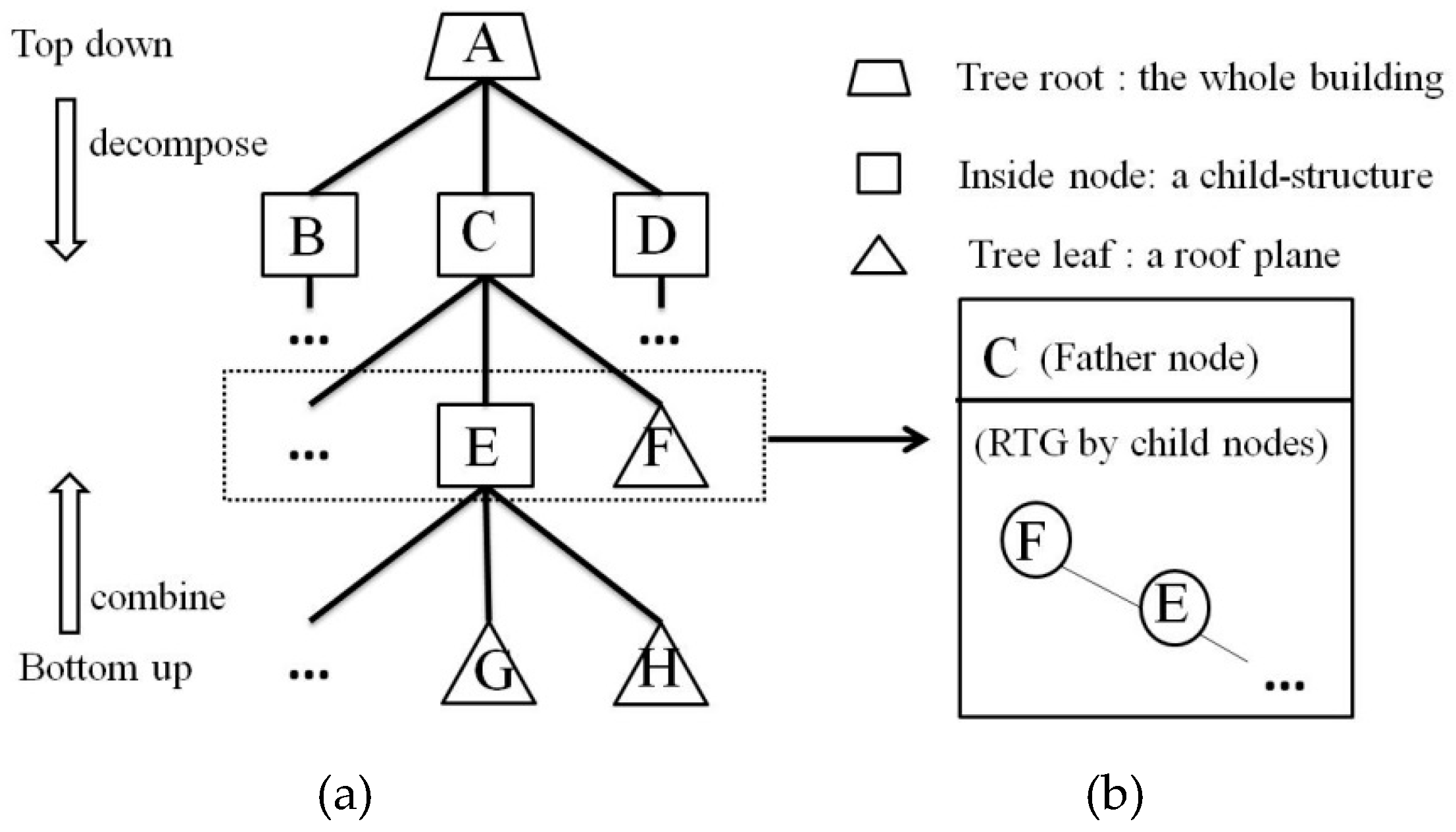
Our new topology structure contains two major parts. One is a multi-way tree structure to organize not only the roof planes, but also those possible child structures within the model. As shown in Figure 3, the roof planes are taken as the leaf nodes and the tree root stands for the whole model. Other inside nodes represent the child structures of the model: the closer to the tree root, the larger/coarser the child structure it represents. Another part is the simple RTGs created together with the tree structure. For each inside node in the HRTT, a simple RTG is generated whose graph vertices are its child nodes. For instance, primitive C contains child nodes such as E and F, and all of its child nodes consists one simple RTG. Such a mixed structure is used to replace the traditional RTG when we construct the roof topology.

As discussed in Section 2, we adopt a progressive approach when constructing the roof topology. Robust connections are detected preferentially and we test whether those connections can be used to reorganize the roof planes. Both top-down and bottom-up strategies are considered: if the model can be easily divided into several parts, we decompose the father node, i.e., Node A is decomposed into B, C, and D; when several planes are strongly relative and can be combined together, we take a bottom-up procedure by constructing the sub-structures locally and projecting their points into the main structure, i.e., nodes G and H are combined into Node E. In this way, those inside nodes are created. Once an inside node is determined, the corresponded simple RTG can also be created by simple graph operations. For instance, if plane G or H is connected to plane F, then Node E and F are connected in the simple RTG of Node C. Those simple RTGs take the child structures as unique vertices and can represent well the integral constraints in the building locale. For the error-prone connections, they will be guided by those constraints or extra verifying process and determined under a hypothesis-verifying process.

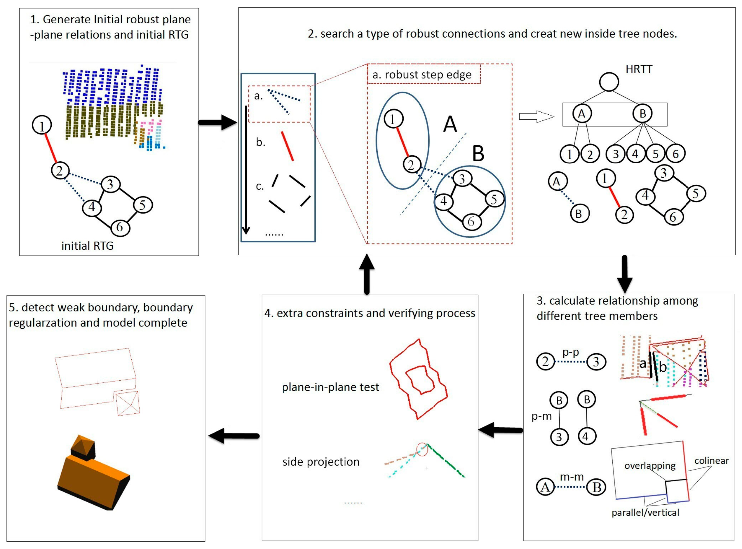
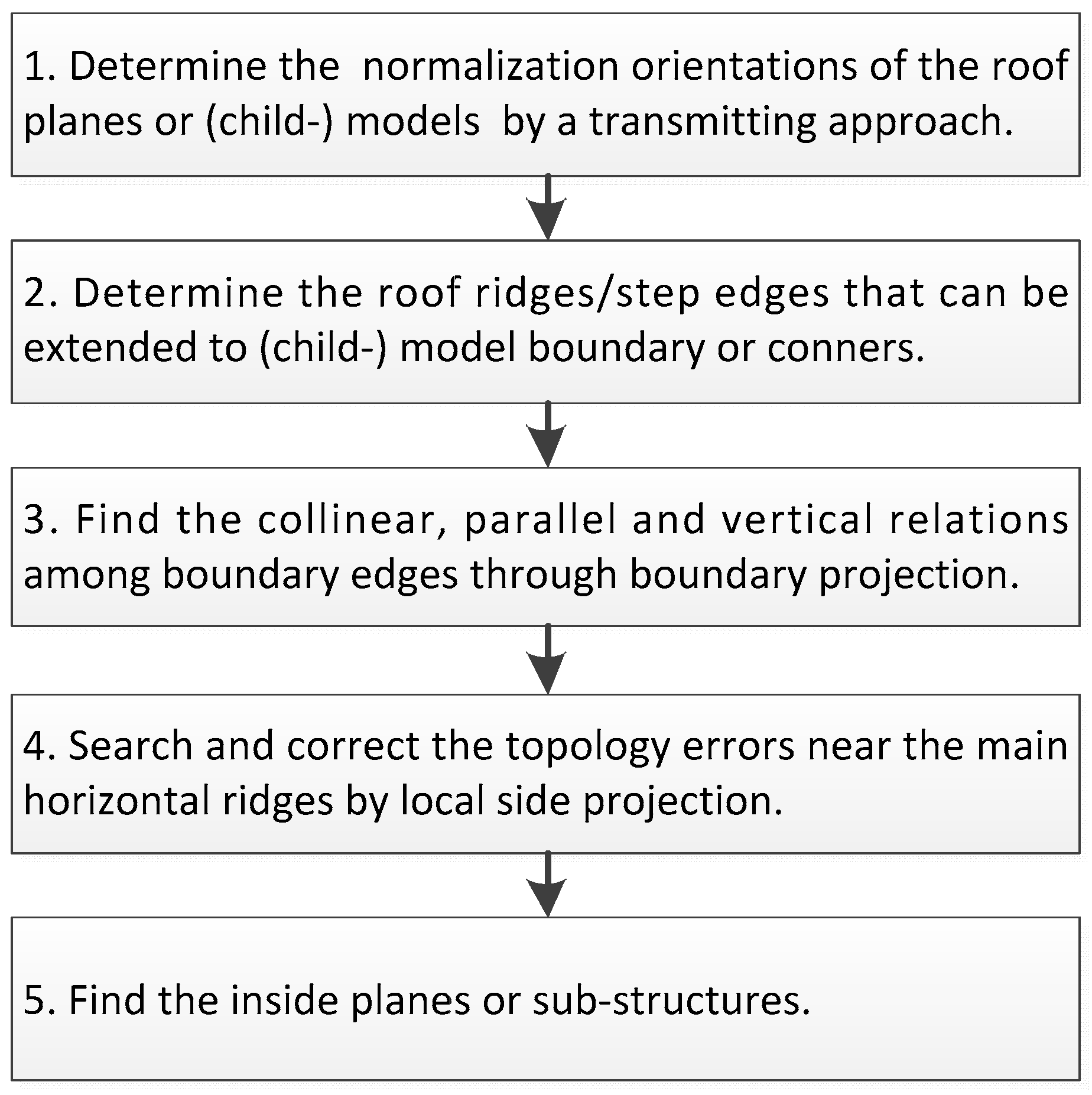
Based on the above idea, a roof reconstruction strategy using the HRTT can be provided in Figure 4. Steps 2 to 4 are repeated, which make the reconstruction process a progressive approach from robust connections to difficult ones. In Section 3.2, we discuss the relations among different tree members and the use of extra information for better topology results (for Steps 1, 3–5), followed by the consideration on inside node determination in Section 3.3 (for Step 2).

3.2. Topology Relations in the HRTT

This section introduces how we describe the relations among different tree members. This not only explains how we organize higher levels of semantic information for better topology results, but also provides the necessary features or information when we determine the inside tree nodes. Three types of topology relations are considered instead of only simple plane–plane relationships in the RTG.

3.2.1. Plane–Plane Relations

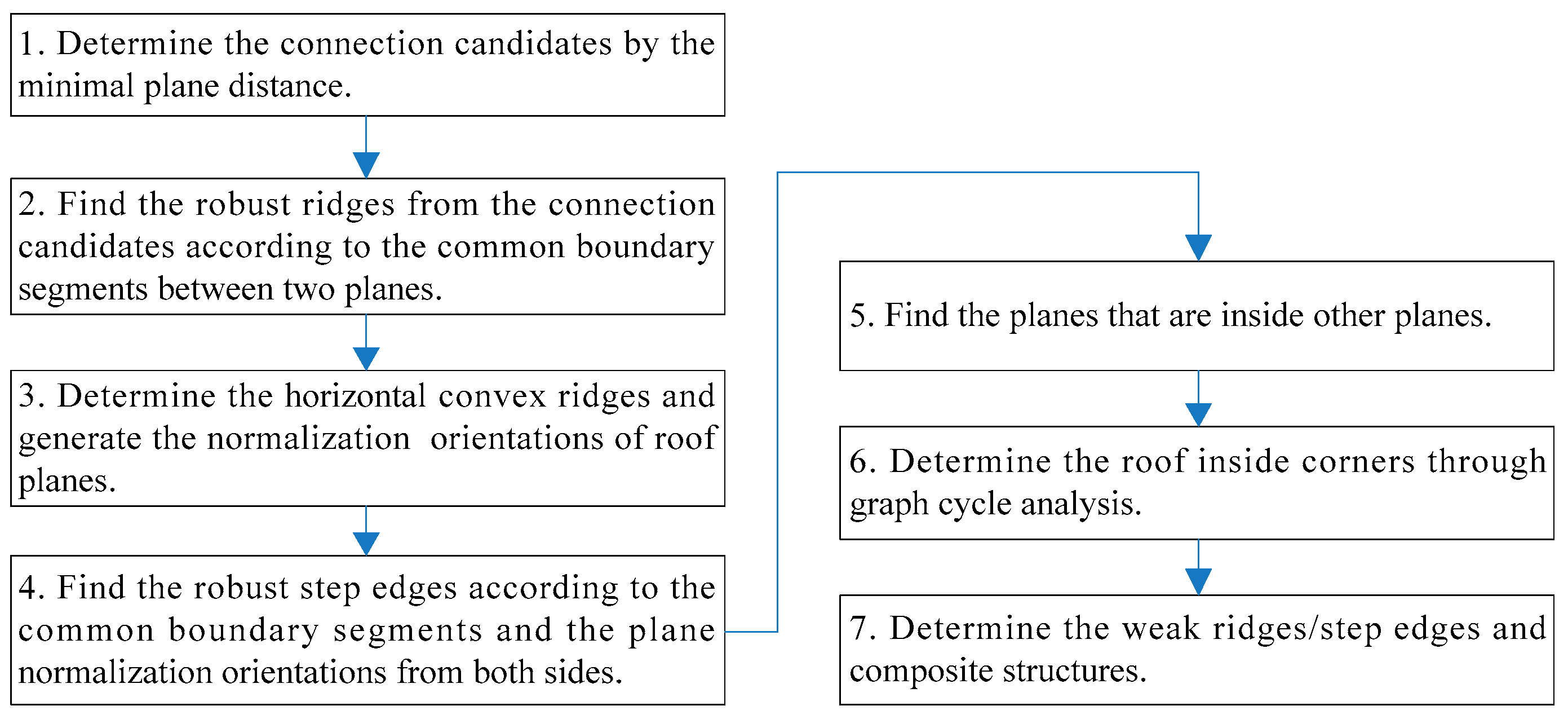
The HRTT adopts a progressive approach that detects connections from robust to error-prone ones. The procedure is provided below in Figure 5.

Our detection of robust connections have referred to many current works: the connection candidates are decided by the minimal plane distance defined in [9], where TIN (Triangular Irregular Network) edges that connect points from different roof planes are tested; for robust ridges and step edges, we use a plane boundary segments based method similar to [31] and the alpha-shape boundary [32,33] is generated to represent the roof plane boundary; the graph cycle analysis [8,10] is used to find the model corners. The robust connections are reliable under strict thresholds or conditions and so are not discussed further. In the HRTT, we mainly concentrate on two issues: the identification of complex connections, such as composite structures discussed in Figure 2; and the detection of weak or error-prone connections from false ones.

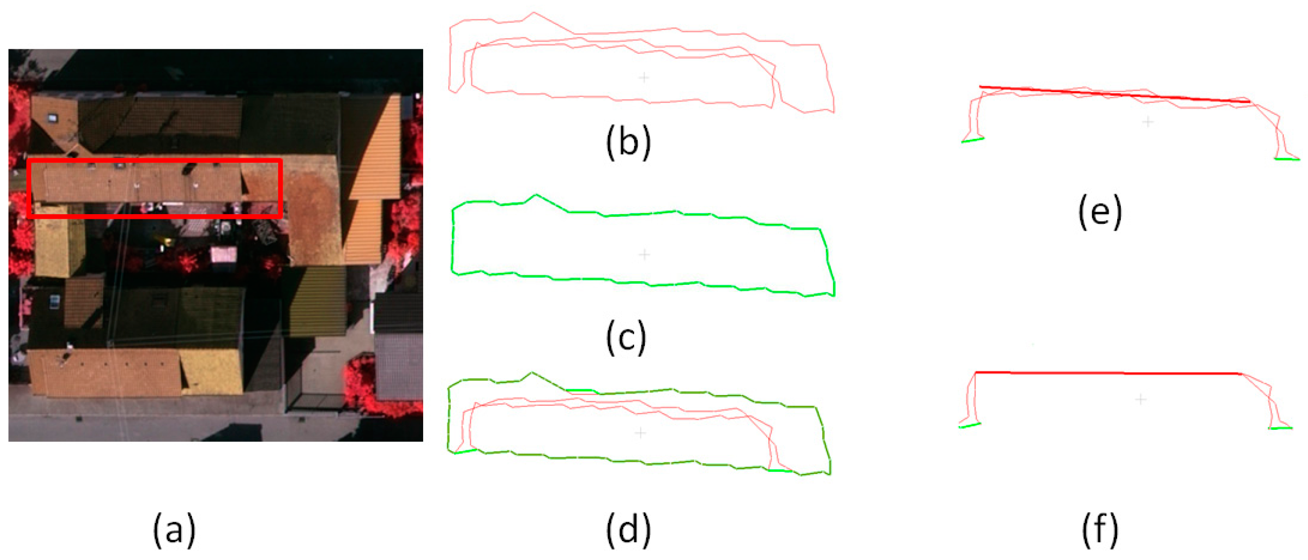
To describe the complex connections, we choose the boundary segments-based method and claim that each supposed ridge/step edge should correspond to a boundary segment. As shown in Figure 6, once reflected to the plane boundary segments, a complex connection cannot be respected by a simple ridge or step edge and, thus, divided into several parts accordingly. If the undecided boundary segments are significant enough (Figure 6f), other additional edges will be considered. An ambiguity here is that the undecided boundary could be caused by improper segmentation results instead of omitted step edges. As such, we need to verify the quality of supposed intersection line or step edge.

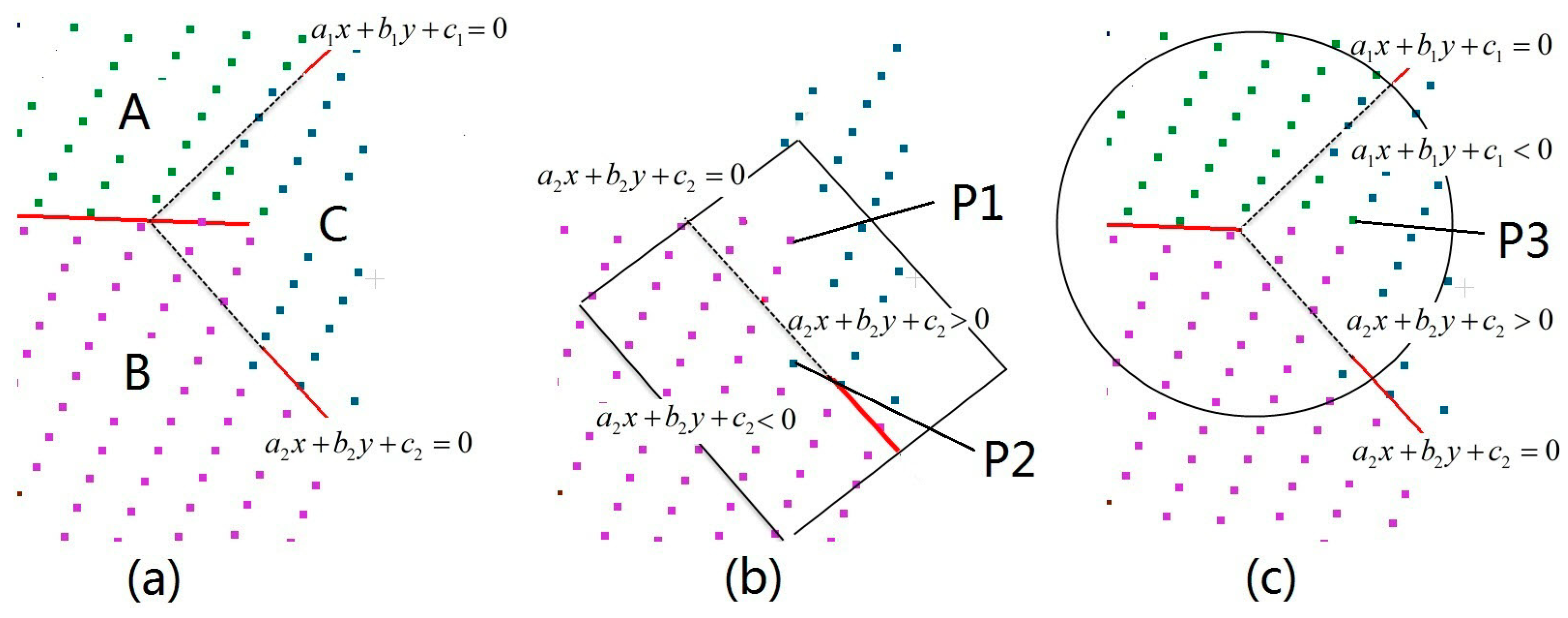
The goal is realized by firstly finding the possible “abnormal” points and then testing whether those points are aggregated or significant enough. We first define the region we considered when searching the abnormal points. In Figure 7, points near the target ridge/step edges are projected to the XOY plane and we only examine them within the 2D region. For relations between only two planes (Figure 7b), the searching region is similar as the buffer area we used when determining the roof ridges, but wider (2 m in each side). For relations among multiple planes (Figure 7c), the region is a circle near the supposed model corner, whose radius is the maximal value of 2 m and the lengths for the three original ridges to be extended to the corner.

Once the searching region is decided, the 2D dividing lines will separate the determining regions into several parts, and each part corresponds to a certain roof plane. Then, for each point in the searching region, we decide whether it is “abnormal” under the following two steps. One is to test if the point is divided into the target region. As shown in Figure 7b, Point P1 belongs to Plane B according to the segmentation results, while it is divided into Plane C by the red dividing line. Points P2 and P3 have the same conditions as P1 and are also set as the candidates of abnormal points. The second step is to test whether the candidates are accepted by the new region. The point-plane distance is taken as the standard here and, if the value is over the predefined threshold (0.2 m), an abnormal point is detected. Those abnormal points are clustered into connected groups by a simple growing algorithm, where a point can grow to another if their spatial distance is smaller than triple the average point distance. Finally, if more than three connected abnormal points are found in one group, the supposed line cannot respect the connection and new connections need to be considered. Based on the above procedure, the three ridges in Figure 7 (Figure 2, also) will be refused to be intersected into the corner even if the graph circle is detected, and new step edges will be considered.

For weak or error-prone connections, our efforts concentrate on the utilization of constraints derived from robust structures and the extra verifying processes in the building locale. As those processes often refer to the relations between roof plane and the child structure to which it belongs, we describe them in the plane–model relations. Additionally, when the height difference between two planes of a step edge is not significant enough, or when segmentation error exists, it is possible that a false short ridge is still detected. As a result, if a long plane–plane connection only contains a very short ridge, we also consider the use of a comprehensive step connection instead of composite structures. The abnormal points defined above are used to evaluate the quality of the new step edge.

3.2.2. Plane–Model Relations

To be manmade objects, the building roof planes have many common features or hidden constraints. Those important information and knowledge are often not fully exploited by simple plane–plane relations. This section will explain how we reflect them into the plane–model relations in the HRTT for better topology results. The issues we considered are provided in Figure 8.

For current methods, in order to distinguish the roof features or normalize the plane boundary, an orientation needs to be estimated beforehand, i.e., the building-dominant orientation. When several adjacent buildings are processed together or when the building structure is complex, a single orientation for them all might be improper and cause over-regularization. In our work, an orientation transmitting procedure is adopted firstly. Initial orientations are produced by the robust horizontal convex ridges and similar orientations are grouped together. Planes containing those robust ridges generate the orientation immediately. Other disorientated planes receive the orientation based on a growing process within the initial RTG. We permit a disorientated plane having more than one orientation and select the best fitting results when multiple orientations exist. If no horizontal convex ridges exist in the model, we estimate it according the boundary of the whole model. The Douglas–Peucker algorithm [34] is adopted to find the edge corners here, and we extract the longest edge segments between adjacent corners, whose points are fitted to produce the orientation of the whole model.

Once the plane orientation is decided, we consider the boundary relations between each plane and the whole child model. By methods similar to Figure 6, we divided the integral boundary into segments where each one corresponds to one roof plane, thus deriving the plane pairs that are adjacent at the model boundary. The boundaries of the holes in the whole child model are also considered as “outside” here. If a roof ridge or step boundary between two adjacent planes has already been detected, we test if they can be extended to the outside boundary of the child model. Such a work is similar to the use of the outermost circle in [10] and, for our methods, the child structure boundary can also be normalized. If no connections are detected, we’ll guess a ridge or step edges according to the boundary height difference. The number of abnormal points defined in above section will be also considered. In this way, some short/weak connections near child model boundary can be decided. For instance, if parts of the four oblique ridges in Figure 9d are lost by the local analysis when discussing the plane–plane relations, they can still be generated here as the supposed ridges can separate the roof points well.

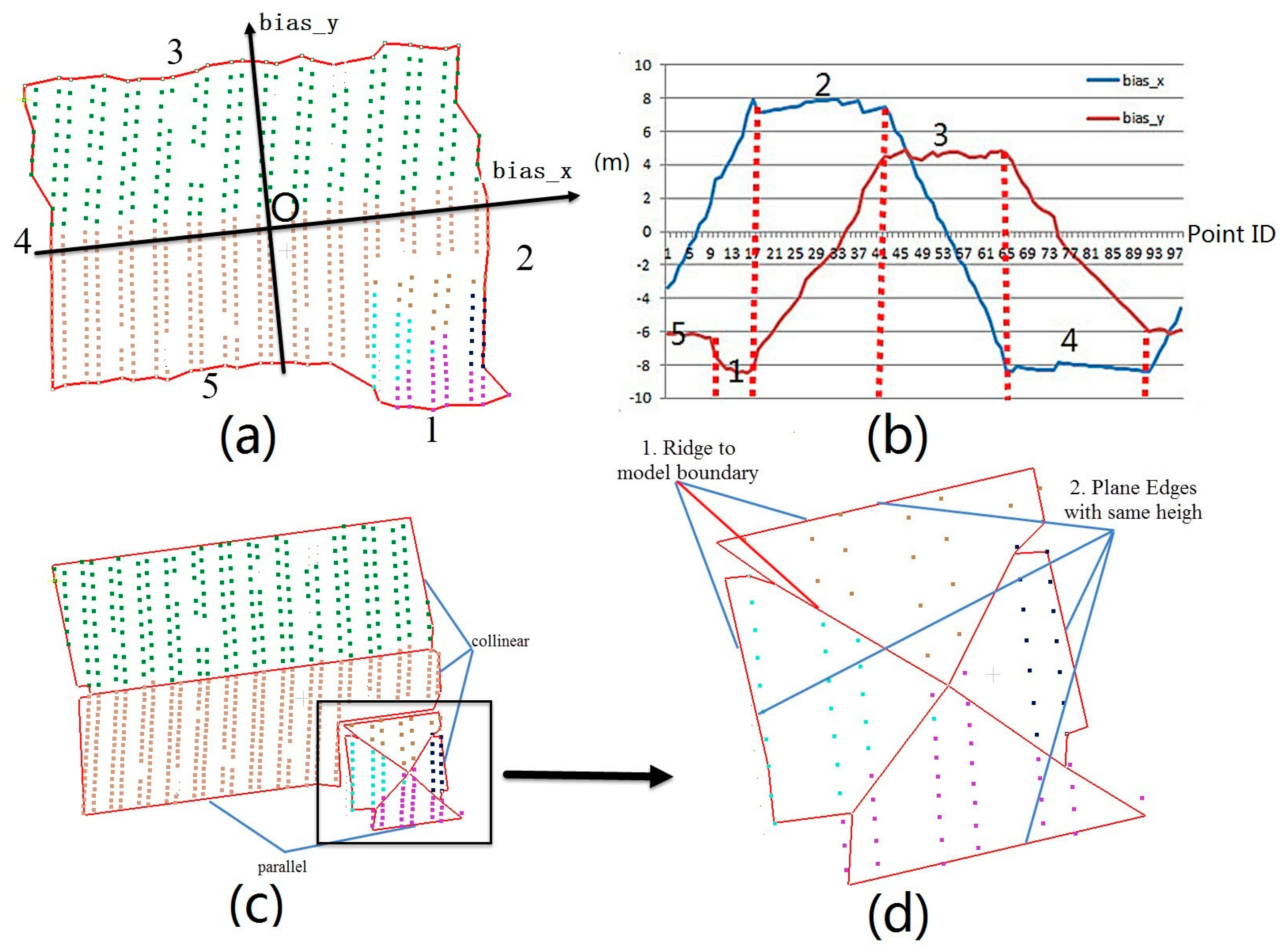
For some RTG-based methods, the plane boundaries are detected within single planes; thus, the collinear/parallel constraints between neighbor planes might be lost. For planes within the same child structure, we use a boundary projection process upon the integral boundary to generate those constraints. As shown in Figure 9b, the integral boundaries are projected to the dominant orientation and its vertical orientation. Then, we claim that the three edges belong to Segment 2 should be collinear and edges in Segments 1 and 5 should be parallel. The boundary projection process is also adopted when we consider the model–model relationship for collinear boundaries. It should be noticed that we store those constraints in a graph structure, as they might be related to each other and need to be calculated simultaneously. For instance, the ridge-to-model-boundary relation in Figure 9d implies the two plane edges having same height. The four ridges will produce four similar relations and eventually conclude that the four edges have the same height.

Side projection is also an effective approach to distinguish the conflicting structures near horizontal convex ridges, especially when the roof window occupies points from the main structure and cause false edges. The approach has already been used for segmentation by work of [30] and shows its advantage in many scenes. In our work, the method is used to recover the local topology errors, i.e., Figure 10. As we only use a local projection, the process is adaptive even if the whole building has multiple normalization orientations.

We also test whether a plane/child structure is inside a main roof plane. This is mainly realized through a point-in-polygon test. Generally, the polygon is defined as the main roof plane’s boundary edge list, and we define an inside plane if all its boundary points are within the polygon. If more than one connected plane is entirely inside the same main roof plane, we consider them together as an inside child structure. For each child structure, we add an inside node in the tree structure of HRTT and search the model primitives to construct it integrally. Additionally, if a plane is only connected to the main roof plane (degree of vertex in initial RTG equal to 1), we use the convex hull of the main roof plane instead of the alpha-shape boundary in case of a roof window is at the roof boundary, where a certain percentage of overlap area (60% of the sub-structure) is demanded. Inside planes or child structures are constructed locally and we project their points to the main structure to construct the entire main roof (Figure 10c). Such a projection process can be very important for the main structure when its point density is sparse and occluded by windows.

3.2.3. Model–Model Relations

For many model-driven methods, the models are completed separately within sub-graph of the RTG or building primitives, which leads to a lack of integral constraints between building primitives. Once inconsistency occurs, i.e., two primitives have different normalization orientations or a short step boundary fails to be detected, holes will appear in the constructed models. In our HRTT, those issues are well considered in model–model relations. The work flow is given below:

When distinguishing model–model relations, points from the same child model are taken as a whole and similar approaches can be adopted, similar to what we do when considering the plane–plane relations. Firstly, the integral common boundaries between two child models are calculated using a boundary comparison process similar to Figure 6. As a model–model connection often refers to several plane–plane connections, we use a simple graph operation to find the set of relations that connect planes from two different child structures. Second, we test the consistency between the integral connection and the corresponded short connections. Just like in the deciding of composite structures in plane–plane relations, we claim that each edge boundary segment should correspond to one short ridge or step edge. The detected conflicts often indicate the short or weak connections that failed to be explored or the inconsistency between the two sides of the child structures.

In the third step, the integral boundary is normalized by boundary projection and we constrain the short edges by the integral edge to generate consistent primitive connections. Once the normalized integral boundary is decided, building primitives from its two sides are extended to the common boundary; thus, the possible holes between two primitives can be avoided. It should be noticed that, if multiple orientations between two primitives exist, all orientations are considered to generate the best fitting one. Additionally, the outside boundary of the entire two child structures will also be considered, just like we do in plane–plane relations, and the parallel and vertical constraints are generated. Finally, the model-in-model test is used on the sub-models inside the main structures, which is similar to the plane-in-plane relations and are not further discussed.

3.3. Inside Tree Node Determination

As claimed in Section 3.1, HRTT literally searches typical types of connections that can derive the inside tree nodes, where both top-down and bottom-up strategies are considered. The top-down strategy keeps searching those robust connections that can easily decompose the model into several parts, such as the robust step edges or main horizontal ridges [35]. The bottom-up strategy gathers the relative planes into the same group, which is similar as the searching of building primitives or sub-structures. Each time we add a type of inside nodes, we consider the plane–model and model–model relations to keep the integral consistency between different tree elements.

To decide a certain type of nodes, we need to refer to the topology relations among the corresponding tree members, where different calculations or decisions need to be taken. For instance, to derive the tree nodes by robust step edges, we first ignore the step connections in the initial RTG (step 4 in Figure 5) and calculate the connecting child graphs. Each child graph is taken as a node to be added. Then, we calculate the integral step boundary between adjacent child structures and compare it with the plane–plane step edges (Steps 2 and 3 in Figure 8) to keep their consistency. Next, each part is constructed separately and expanded to the common step boundary, if necessary, knowing that those step boundary may be changeable in the follow-up steps (Step 3 in Figure 11).

Table 1. Topology relations considered when deciding inside tree nodes in the HRTT.

Connection Type	Plane–Plane (Figure 5)	Plane–Model (Figure 8)	Model–Model (Figure 11)
Robust Step edge	4	2, 3	3
Main horizontal ridge	2, 3	2, 3, 4	2, 3
Edges to model boundary	6, 7	2, 3	2, 3
Sub-structures	5	5	3, 4

provides the connection type we considered and the message it needed when considering the relations among different tree members.

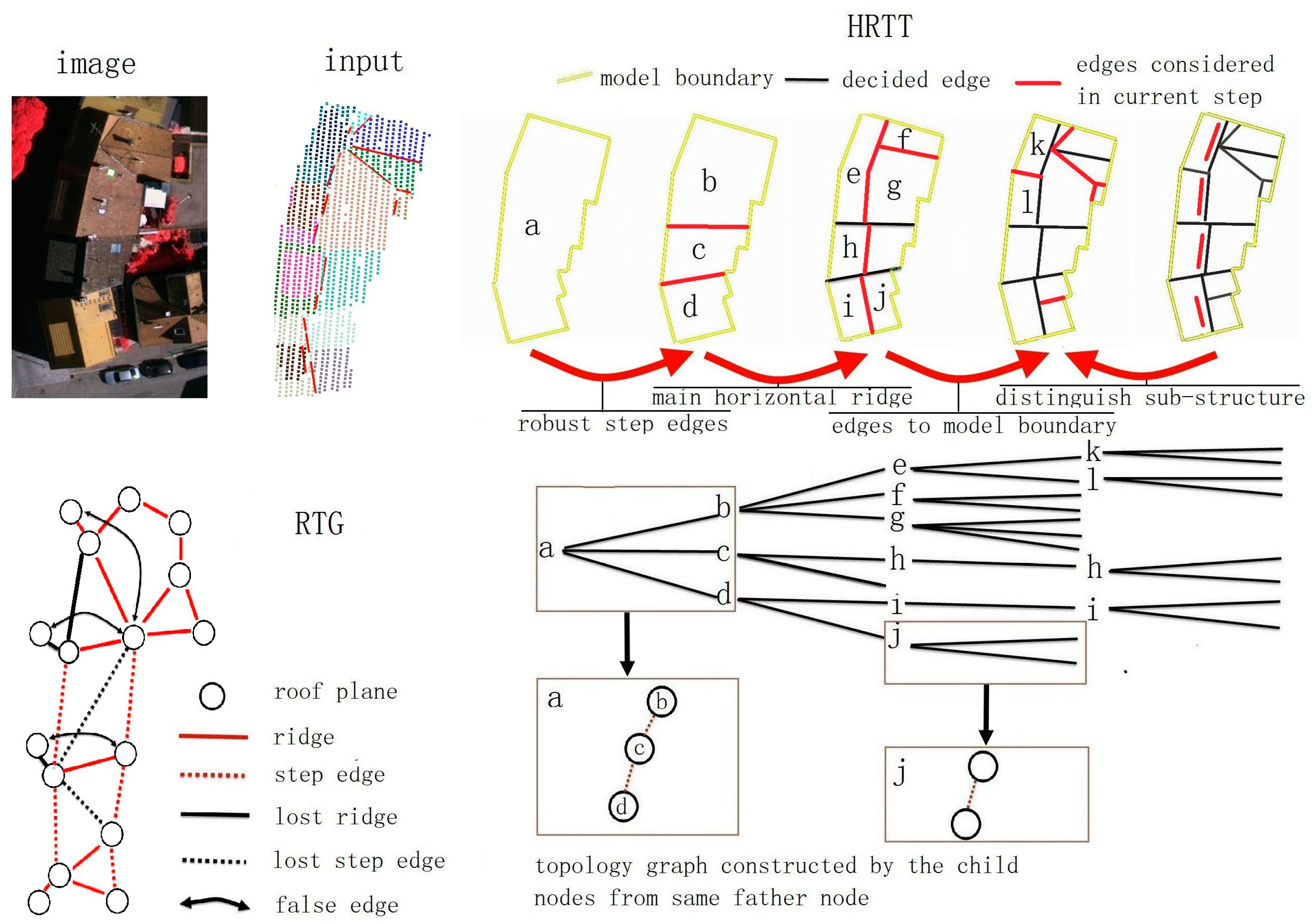
For better understanding, Figure 12 gives an example of the hierarchical construction procedure we realized based on the HRTT. It shows how we add the inside nodes and dividing the roof planes step by step, and also indicates its difference with traditional RTG-based methods. The area is selected from Area 1, the ISPRS benchmark data [36]. Current RTG-based methods confront a large number of challenges in this data: The regularization orientations are difficult to decide for the child structures (b has two orientations, c has irregular edges connected to building d); the existence of large bay windows makes the point density of the main structures sparse and causes false edges with the opposite planes; the small plane in f may also be omitted in segmentation results. By calculating the common features integrally, the lost step edges can be generated under the consistency test (i.e., the step edges between h and j). The main horizontal ridges divide the roof planes into its two sides and the use of side projection can avoid the false ridges (i.e., in child structure c). For the omitted plane in f, the error will be limited within the child structure that can be easily repaired in the follow-up approaches. As a result, the final topology results are greatly improved.

It has to be noted that we never limit the types of child structures or the depth of the tree. Thus it is possible to add in new type of inside nodes when necessary, such as the wall planes. Additionally, if we failed to generate some inside nodes, no extra errors will be brought in and we can process it just like traditional methods. Particularly, when no inside nodes are found, the HRTT is simply the same as the traditional RTG, thus the RTG can be taken as a special case of the HRTT.

4. Experiments and Discussion

This section presents the overall performance of the proposed methods experimentally. Various assessment metrics are used to assert the methods and the results are compared with current studies to prove its robustness.

4.1. Datasets, Reference, and Parameters

Two datasets are used in our experiments: one is collected from the city of Vaihingen, the benchmark data of the “ISPRS Test Project on Urban Classification and 3D Building Reconstruction”, which allows us to use external reference data [36]; another is the Wuhan University data, with higher point density, introduced in [37]. The properties of the two datasets are provided below in

Table 2. Properties of the two datasets.

Site	Vaihingen	Wuhan University
Acquisition Date	22 August 2008	22 July 2014
Acquisition System	Leica ALS 50	Trimble Harrier 68i
Fly Height	500 m	1000 m (cross flight)
Point Density	~4/m2	>15/m2

. In our experiments, we construct the roof topology from the segmented roof points, and more details about the LiDAR point cloud segmentation may also refer to our recent work [37].

To evaluate the precision of the reconstruction algorithm, two groups of manual references are used in quantitative experiments. The first group is for the topology precision, which considers only the connections between plane pairs. For a plane–plane connection, two planes should be both found in the reference first, and a least overlap of 50% needs to be ensured. Then, two indices are considered: one considers the existence of the connection, and the other considers the similarity between the connection and the reference. The segmentation results upon Area 1 of the ISPRS benchmark data are selected as the input data, where 185 ridges and 81 step edges are defined in our reference. For step edges we only consider the 2D precision and as for a composite structure, we will only assert the ridge part. For more detail information, the readers may need to refer to our recent work [37], where the quantitative standard and the segmentation results are all clearly provided. The second group is from the ISPRS test project [36] and evaluates the model reconstruction results by the roof boundary polygons. Since this is a test dataset from a third party, it is only possible to compare the DSM images and some other quantitative results. In the references, the three test areas have 37, 14, and 56 buildings and 288, 69, and 235 planes, correspondingly.

The platform of the compute program is based on an open sources project, Cloud Compare [38], which provides basic algorithm I/O, such as data reading/writing and model displaying, as well as simple statistics or operations upon the point clouds. The platform supports multiple operating systems and our work is developed on Windows 7, using C++ under VS2010. Some open source algorithm libraries are also included, such as the PCL [39] for point neighborhood analysis and the CGAL [33] for the alpha-shape edges. The main parameters used in the proposed test area are shown in

Table 3. Parameters used by the proposed method.

Parameters	Vaihingen	Wuhan University
Input point cloud examine
Minimum number of points for a building	50	200
Minimum number of points for a roof plane	5	20
Maximum slope for a roof plane	80°	80°
For ridges/step edges (Section 3.2.1)
Minimum ridge/step edge length (robust)	1 m	1 m
Minimal height difference for step edges (robust)	0.5 m	0.5 m
Buffer width near the roof ridges	1 m	1 m
Small angle (for deciding horizontal/collinear ridges)	3°	3°
For boundary
Scale for alpha-shape edge detection	3AveDis	3AveDis
Minimal spacing between two adjacent parallel edges	1 m	1 m
Minimal number of points in an edge segment	3	5
Distance threshold for Douglas–Peucker algorithm (Section 3.2.2)	0.15 m	0.15 m
For abnormal points/area (Section 3.2.1)
searching radius/buffer width	2 m	2 m
Point to plane distance threshold	0.2 m	0.2 m
Distance threshold for adjacent abnormal points	3AveDis	3AveDis
Minimal number of adjacent abnormal points	3	10
Minimal overlap for plane-in-plane test (Section 3.2.2)	60%	60%

Notes: the AveDis is the average point distance, established automatically.

.

Most parameters have already been introduced in Section 3, which are marked and not further discussed here. The rest parameters mainly concentrate on two aspects. The first part is to examine the input data, including the size of roof planes and buildings. As we only consider the rooftop, the slopes of planes are also controlled, in case of the conflicts caused by the projection approaches. Additionally, we suppose that the connectivity of roof points in plane segments have already been ensured in segmentation results; thus, the alpha-shape edge can be generated smoothly. The other part is for the boundary projection approach we used to normalize the roof edges. The major issue here is to balance the demands between precision and normalization. The minimal spacing between two nearby parallel edges decides whether the two should be combined into one. The minimal number of points in an edge segment decides whether the local edge details should be omitted, and can avoid the zigzag edges caused by boundaries that are not consistent with the domain orientation.

4.2. Model Reconstruction Results

4.2.1. Vaihingen

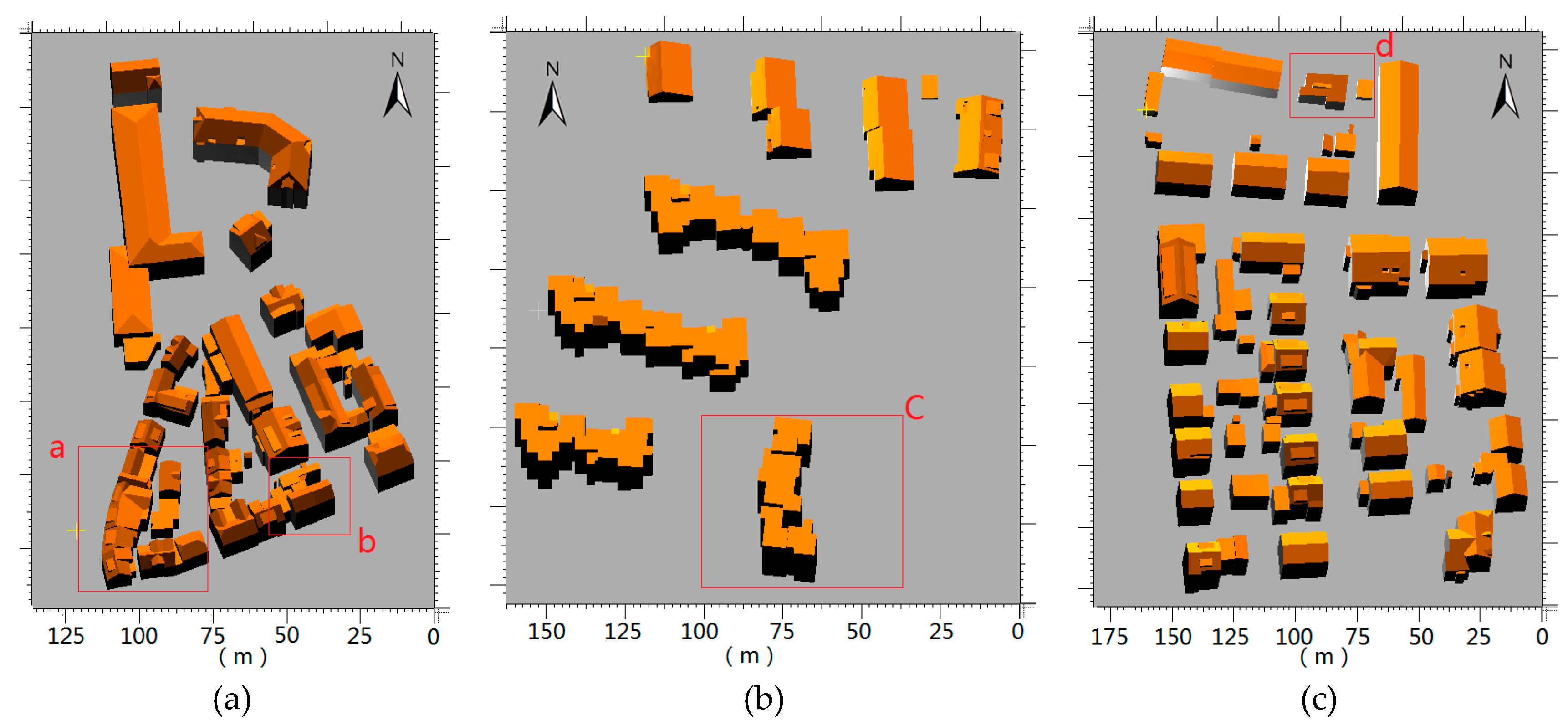
Figure 13 shows the results of the three test areas in the Vaihingen, ISPRS test dataset, which are widely adopted and compared by current studies. Area 1 contains dense development, consisting of historic buildings having complex shapes. Especially for the lower-left parts, several buildings have different normalization orientations, irregular outside boundaries, and large windows that occlude the main structures, which create problems for the current methods. Area 2 is characterized by high-rise residential buildings surrounded by trees. The roof boundaries are very complex, and the gaps between adjacent roofs have large height differences. Area 3 is purely residential, with detached houses surrounded by trees. The reconstruction results show the adaptation of the proposed method. We have uploaded the results to the ISPRS test project [36,40], and the comparison of the quantitative results with four other state-of-the-art studies will be discussed latter.

4.2.2. Wuhan University

Figure 14 shows the reconstruction results of the Wuhan university dataset, with a much higher point density. As the data is generated through cross-flights, it is more variable locally, as two close points (with similar x and y values) from different flights may have relatively larger height difference. Additionally, the scales of roof plans change largely from the main structures to small local details. This brings much challenge to the current methods, not only to the adaptation of the feature extraction methods but also the selections of algorithm thresholds. HRTT shows great adaptation under those various situations as it decomposes the complex scenes into child structures step-by-step, while maintaining their interrelations simultaneously. From the results of the constructed models, it can be seen that our method can construct very complex model types and maintain the small roof details simultaneously. Furthermore, the consistency among different model primitives is well kept and the parallel/vertical constraints are ensured.

4.3. Precision Analysis and Limitations

This section proposes the performance and limitations of our proposed HRTT, in quantitative and qualitative terms. Both topology correctness and model precision are evaluated and compared with RTG-based methods, which is followed by a discussion on the limitation.

4.3.1. Topology Precision

Table 4. Description of local analysis methods adopted in the RTG-based method.

Method	Roof ridge	Step edge	Parameters (e.g.)
Type A: by point- point connections [9]	Minimum distance of all point combinations (dmin)	Degree of r-vertex (r = 1), detect by boundary tracing	dmin = 1 m;
Type B: by point counts near the feature lines [6,8,10]	Points count within buffer area (nPt) and minimum ridge length projected by points (Lmin)	Nmin points within planimetric distance dmax, but larger height difference than Hmin	nPt = 10; dmax = 1 m; Lmin = 0.5 m; Hmin = 1 m;
Type C: by roof boundary edge segments [7,31]	Common boundary edge segments within buffer area (Bdmin), ridge length projected by edge (Promin)	Edge pixel chain is split into 2D and test the 2D boundary length	Bdmin = 1 m, Promin = 0.5 m; (Our_initial: Promin = 1 m)

Notes: our robust connections are detected by similar methods as Type C, but stricter thresholds. The width of the buffer area is set as twice the point distance.

concludes three major types of local analysis methods used in current RTG-based methods that distinguish the roof topology. A brief description about their realization and the used parameters are also provided. We compare the HRTT results with those methods to evaluate its performance and robustness. The evaluate methods and the references data we used have been introduced in Section 4.1, and the topology precisions are provided below in

Table 5. Performance comparison of different topology identification methods.

Topology Precision		A	B	C	Our_initial	Our_final
RTG based	compl (%)	90.3	88.4	85.8	84.5	92.9
	corr (%)	85.0	92.6	93.0	94.9	96.0
	qua (%)	78.8	82.5	80.6	80.9	89.4
ic > 0.3	compl (%)	90.3	87.1	85.2	83.9	91.6
	corr (%)	84.0	91.8	93.0	94.2	95.9
	Qua (%)	78.0	81.1	80.0	79.8	88.2

Notes: RTG-based precision cares only about the existence of plane–plane connection, while the index ic [37] also considers the quality of edge by comparing it with the reference. compl: completeness = TP/(TP+FN); coor: correctness = TP/(TP+FP);qua: quality = TP/(TP+FN+FP), where TP (true positive) is the number of objects found both in the references and results, FN (false negative) is the number of reference objects not found in results, and FP (false positive) is the number of detected objects not found in the reference. Our_initial is the precision of our initial RTG-distinguished results, using the Type C method, but with stricter thresholds (Table 4). Our_final is the precision of the final precision after HRTT is constructed.

.

Local analysis methods need to make a balance between the completeness and correctness. Looser conditions can detect the weak/short roof ridges, while the possibility of bringing in false edges will also increase, and vice versa. As a result, Type A receives the highest completeness, but the lowest correctness. For HRTT, the robust connections are detected preferentially (high correctness), and we permit some weak or error-prone edges to be undecided (low completeness). Type C conforms to such demands and we use a stricter threshold for it to generate the best initial correctness. As extra constraints and the verifying procedures are adopted in the follow-up steps, both completeness and correctness in our final HRTT results are improved. Considering that local analysis results may be influenced by thresholds and the used methods, we select 10 error-prone connections in Figure 15.

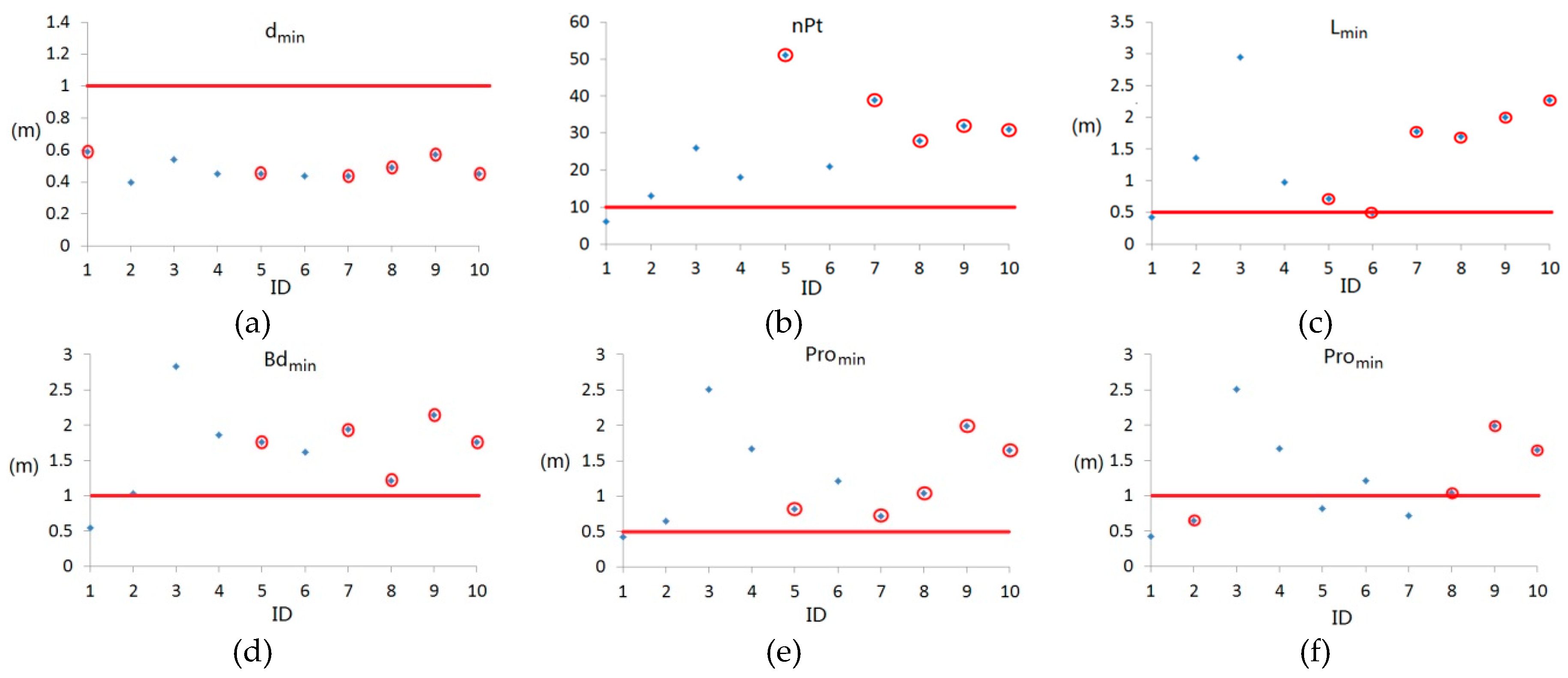
For Positions 2, 4, and 6 in Figure 15, the amount of roof points near the reference ridges are very small and the roof edges nearby are hard to find. As a result, the ridges can easily be lost under strict thresholds or improper segmentation results. In our work, ridges in 2 and 6 will be re-extracted when considering the plane–model relations, even if they are lost here. The reason is that the two planes of the ridge share a connected boundary segment of the (child) model, while no connections have been detected. Our algorithm will guess a roof ridge here (discussed in Section 3.2.2) and extend it to the model outside the boundary if the new ridge is accepted. The ridge in 4 can also be corrected because a four-vertex circle is found around it and cannot produce a corner, and the two possible ridges that decompose the circle into two triangles will be examined. In Positions 5, 7, 8, and 10, there are no roof ridges in the reference, while the height differences between the adjacent planes are very small near the supposed intersecting lines. As a result, both the point counts and the length of the common edges will be large enough for the connections to be falsely distinguished as roof ridges. An advantage of our methods here is that, even if a roof ridge is detected, we still consider the step parts if the undecided boundary between two planes is significant enough. For a long plane–plane connection that only contains a very short ridge, we consider using a comprehensive step connection instead of the composite structure. For Position 9, the error is caused by poor segmentation results, and our method corrects it by side projection. In Positions 1 and 3, errors were reported in some current researches, i.e. [36], while all methods performing well here thus are not further discussed. The static results of the 10 connections are provided below in Figure 16.

For Type A in Table 4, the d_min of all connections are close to the average point distance and ten connections will all be accepted, either true or false ones. For Type B, some false connections (7–10) even obtain greater point counts (nPt); thus, they can hardly be excluded by simply changing the thresholds. A similar conclusion can also be generated by indices in Type C. As those false connections generate rather statistic values similar to the true ones, a stricter threshold can exclude more false connections (i.e., it can be concluded by comparing the Pro_min values of Connections 5 and 7 in Figure 16e,f) while losing the weak connections (Connection 2). The statistic results prove that using simple local analysis or adjusting the thresholds can never solve the topology problems, and more extra procedures and constraints need to be considered. The final topology precision shows that our strategy is effective.

4.3.2. Model Precision

As introduced in Section 4.1, the quantity results on the final reconstruction models are provided by the ISPRS test project [36]. For our own method, more quantity information is available, and we summarize the precision of the three areas in

Table 6. Detail precision of our method.

Area	Pixel Level			Plane Level				Pixel Level			Plane Level
	TP	FN	FP	TP1	TP2	FN	FP	Compl	Corr	Qua	Compl	Corr	Qua
1	613137	39584	13445	265	199	23	7	93.9	97.9	92.0	92.0	96.6	89.1
2	422093	57492	5765	48	55	21	1	88.0	98.7	87.0	69.6	98.2	68.7
3	754427	57018	18827	203	143	32	5	93.0	97.6	90.9	86.4	96.6	83.9
sum	1789657	154094	38037	516	397	76	13	92.1	97.9	90.3	87.2	96.8	84.7

Notes: The pixel size is set as 0.100 m and the definition of FP, FN, Compl, Corr, and Qua are the same as Table 5, while the TP at the plane level can be slightly different. Table 5 uses the definition of [41] to get one-to-one relations between the tested result and the reference; thus, TPs for completeness and correctness are the same. Here, the definition of [38] is used and two TPs are produced: TP1 for completeness and TP2 for correctness.

. Additionally, four state-of-the-art studies are also selected for comparison and their quality results on major indices are provided below in

Table 7. Precision comparison of the reconstruction results on the ISPRS dataset.

Region	Method	Compl	Corr	Compl_10	Corr_10	1:M	N:1	N:M	RMS(m)	RMSZ(m)
Area 1	CKU	86.8	98.9	88.4	99.2	10	36	3	0.9	0.6
	ITCX3	89.2	96.4	93.2	97.7	5	39	6	0.8	0.2
	TUD2	73.3	100.0	70.7	100.0	1	36	3	0.8	0.2
	YOR	88.2	98.5	94.6	99.2	5	36	14	0.8	0.3
	Ours	92.0	96.6	94.6	98.5	10	36	8	0.8	0.2
Area 2	CKU	78.3	93.1	93.8	100.0	8	4	0	0.5	0.7
	ITCX3	71.0	100.0	89.6	100.0	3	4	1	0.5	0.2
	TUD2	71.0	100.0	89.6	100.0	2	3	0	0.3	0.3
	YOR	66.7	100.0	83.3	100.0	5	3	0	0.5	0.3
	Ours	69.6	98.2	87.5	97.9	6	3	0	0.6	0.3
Area 3	CKU	81.3	98.4	91.9	99.1	4	48	2	0.8	0.6
	ITCX3	88.1	88.2	96.8	95.8	3	50	2	0.7	0.1
	TUD2	73.6	100.0	81.5	100.0	0	42	0	0.5	0.1
	YOR	84.7	100.0	97.6	100.0	2	51	1	0.6	0.2
	Ours	86.4	96.4	95.2	100.0	9	44	5	0.6	0.2

Notes: We use the same method name as the website, where both reconstruction results and methods describe can be easily found. CKU [42], ITCX3 [6], TUD2 [10], and YOR [43] are the short names of the participant. Compl and Corr are the completeness and correctness of the constructed roof planes at object level, and Compl_10 and Corr_10 are the corresponding precision for big planes (>10 m²). 1:M, N:1, and N:M are the topology quality of planes. RMS is the planimetric geometric accuracy: average root mean square distance to reference boundary, in XOY plane. RMSZ is the geometric accuracy and the Z component is the average root mean square distance of the detected DSM and reference DSM.

.

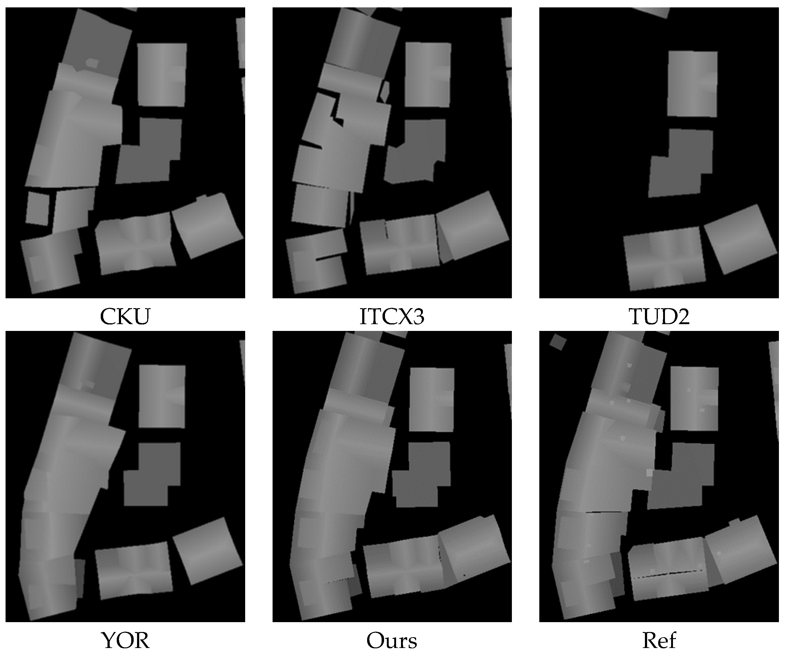
The final reconstruction precision can be influenced by many factors besides the reconstruction strategy, i.e., results of pre-processing, such as building detection and segmentation, as well as the precision and reliability of reference data. Additionally, just like the deciding of roof ridges, we need to find a balance between completeness and correctness. For instance, the correctness values of TUD2 are all 100.0%, while its completeness can be much lower than other methods. As a result, no method seems to be distinctly better than others just by quantitative results. For our HRTT, the hierarchical structure considers the integral structure of whole models, thus, produce better completeness than other methods, while our correctness do not obviously decrease. This also reflects on the constructed building models. So far, only the DSM results of the constructed models are available for other methods and we select region (a) in Area 1 as an example. In Figure 17, it can be concluded that current methods still confront lots of difficulties in the area. For HRTT, the model–model relations ensure the integral connectivity of the whole building, thus, the holes for CKU and ITCX3 can be successfully avoided. Meanwhile, we allow different child structures having their own normalization orientations, thus, the roof boundary is much better than YOR, visually. The detection of main horizontal ridges and the side projection approach can correct the segmentation errors and recovers the right topology under sparse data. As a result, we generate the best performance in this region. In addition, the low completeness of all methods in Area 2 is mainly caused by the small planes of the guardrail in high-rise residential buildings, which are often only one point wide. Those planes are omitted by our boundary edge-based procedure, thus leading to poor completeness. The quality of plane edges can refer to the indices’ RMS in Table 7 and we further exhibit it in Figure 18. Two types of results are provided here. In Figure 18a, we mix the roof boundary with the raw point clouds and the results demonstrate that the constructed edges have good consistency with the initial data. This can also be proved by the pixel-level model precision in Figure 18b, where most areas are well superposed by the reference DSM and the pixel-based quality indices achieve a precision of 90.3% (Table 6).

4.3.3. Limitations

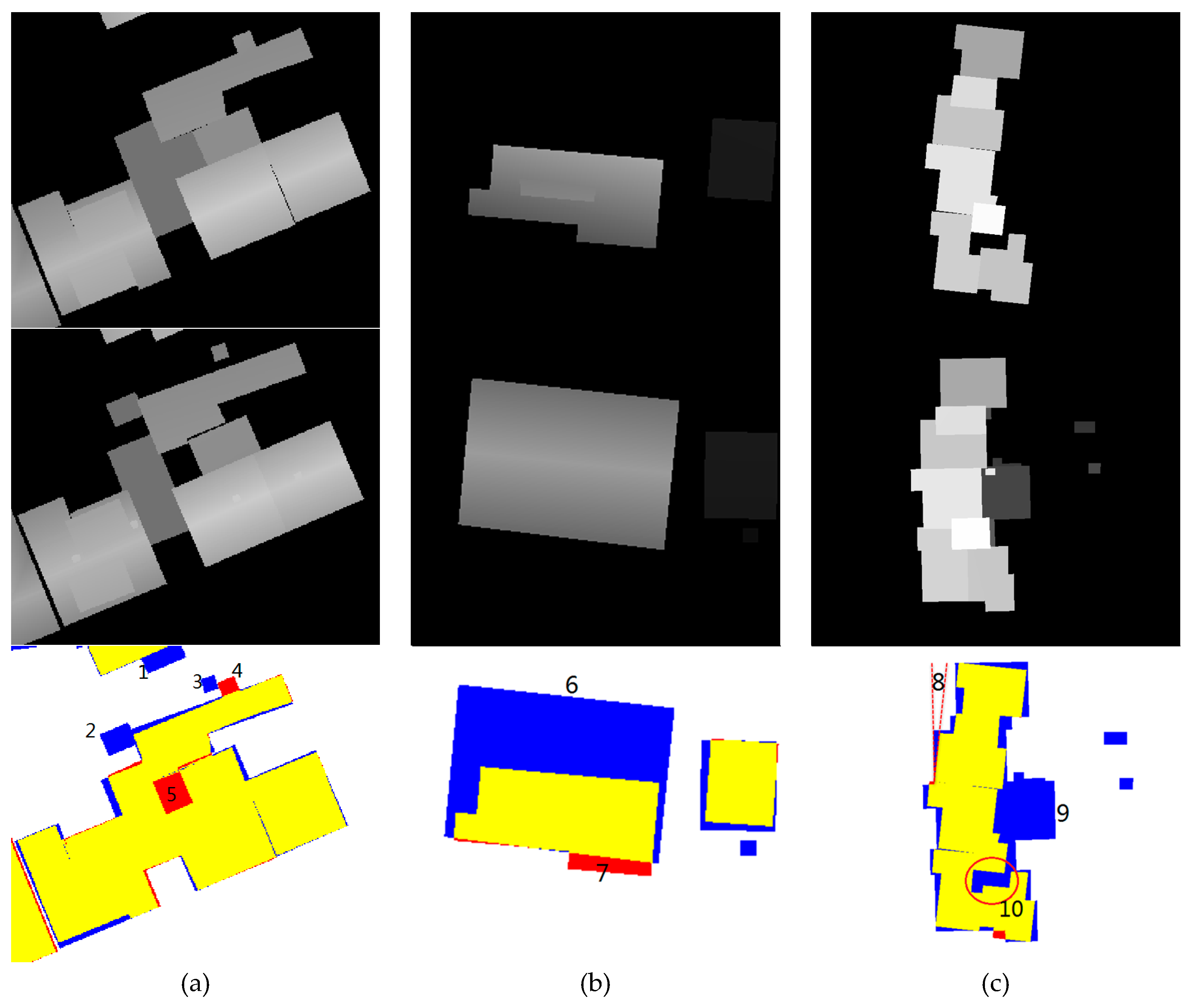
Figure 19 shows some buildings in Vaihingen that can bring troubles to our reconstruction methods. The major issues are caused by errors in pre-processing procedures and the sparsity or lack of data. Figure 19a shows that several small roof planes are lost, i.e., Roofs 1, 2, and 3, which can be caused by errors in pre-processing procedures such as point classification or roof segmentation. Errors in 4 and 7 are caused by vegetation near the buildings. As those errors are caused by preprocessing procedures, both RTG- and HRTT-based methods will fail here. Roofs 5 and 10 should be especially emphasized as it belongs to the inside model holes. In HRTT, we keep the integral connectivity of the whole model. Thus, if the holes are not distinct enough, or smaller than the scale that the alpha-shape boundary can be detected, the holes will be filled by a lower roof nearby. Roof 5 is falsely filled because the vegetation points in the region are taken as building points; as regards Roof 10, no LiDAR point is available here in the raw data. Figure 19b shows the error caused by light absorbing surfaces (roof 6), and the method failed because the data is too sparse. In Figure 19c, our methods perform poorly because the building domain orientation is not well estimated. Generally, our boundary normalization procedure requires a pre-estimated orientation. For most buildings, the orientations are estimated by the main horizontal ridges within the whole building, as the roof ridges have the best precision [44]. If no ridge is available, we simply estimate it through the whole model outside boundary; thus, it can be inaccurate sometimes, especially when the real domain orientation is close to the scan line direction of raw LiDAR data. In addition, there are also other errors caused by irregular curved surfaces or multilayer surfaces, though not discussed here.

5. Conclusions

This work proposes a hierarchical roof topology construct strategy for robust building model reconstruction. The HRTT is adopted instead of the traditional RTG to represent the topology relations among different roof elements. Not only the plane–plane connections but also the plane–model and model–model relations are considered in the HRTT. In allusion to the issues of error-prone connections, we preferentially distinguish the robust features, which decompose the whole model into simpler components step-by-step and produce the basic semantic information to identify the ambiguous parts locally. In this way, the effect from structures of minor importance or spurious ridges can be limited or avoided, and common features and integral constraints can be fully exploited. Those additional features or constraints are distinguished and well-organized, along with the construction of HRTT, which eventually produces better topology results and building models. Experiments on both roof topology precision and the constructed models prove the effectiveness of the proposed approach. Compared with the RTG-based method, two topology quality indices increase from 80.9% and 79.8% to 89.4% and 88.2% in the text area (see Table 5). The integral model quality indices of the three ISPRS test data sets at the pixel level and the plane level also achieve the precision of 90.3% and 84.7%, accordingly (see Table 6).

However, our method has several limitations. First, the construction results can be influenced by the errors of pre-processing processes, such as segmentation, or the imperfection of initial data. Though additional processes, such as side projection, can correct some of the errors, a topology correction process, such as [6], may still be needed and HRTT can provide a local search here. Second, the description of roof topology in our methods only guarantees the completeness in 2D and if two roof planes are partly overlapped in 2D, the overlapped parts from the bottom roof plane will be lost.

There are also some possible improvement directions for future work. First, the HRTT provides a structure that decomposes the whole model into meaningful sub-structures step-by-step. How to decide the construction strategy and parameters under different roof scales becomes an important issue. Second, more pre-defined structures, such as model primitives, can be introduced, which form the robust inside tree nodes in the HRTT. Other additional constraints and verifying processes can also be used to generate highly normalized models.

References

1. Haala, N.; Kada, M. An update on automatic 3D building reconstruction. ISPRS J. Photogramm. Remote Sens. 2010, 65, 570–580. [Google Scholar] [CrossRef]
2. Musialski, P.; Wonka, P.; Aliaga, D.G.; Wimmer, M.; Gool, L.; Purgathofer, W. A survey of urban reconstruction. Comput. Graph Forum. 2013. [Google Scholar] [CrossRef]
3. You, S.; Hu, J.; Neumann, U.; Fox, P. Urban site modeling from LIDAR. In Proceedings of the International Conference on Computational Science and its Applications, Montreal, QB, Canada, 18–21 May 2003; pp. 579–588. [Google Scholar]
4. Vosselman, G.; Maas, H.G. Airborne and Terrestrial Laser Scanning; Whittles Publishing: Dunbeath Mill, UK, 2010. [Google Scholar]
5. Verdie, Y.; Lafarge, F.; Alliez, P. Lod generation for urban scenes. ACM Trans. Graph. 2015, 34, 15. [Google Scholar] [CrossRef]
6. Xiong, B.; Elberink, S.O.; Vosselman, G. A graph edit dictionary for correcting errors in roof topology graphs reconstructed from point clouds. ISPRS J. Photogramm. Remote Sens. 2014, 93, 227–242. [Google Scholar] [CrossRef]
7. Verma, V.; Kumar, R.; Hsu, S. 3D building detection and modeling from aerial LIDAR data. In Proceedings of the 2006 IEEE Computer Society Conference on Computer Vision and Pattern Recognition, New York, NY, USA, 17–22 June 2006. [Google Scholar]
8. Elberink, S.O.; Vosselman, G. Building reconstruction by target based graph matching on incomplete laser data: Analysis and limitations. Sensors 2009, 9, 6101–6118. [Google Scholar] [CrossRef] [PubMed]
9. Sampath, A.; Shan, J. Segmentation and reconstruction of polyhedral building roofs from aerial LIDAR point clouds. IEEE Trans. Geosci. Remote Sens. 2010, 48, 1554–1567. [Google Scholar] [CrossRef]
10. Perera, G.S.N.; Maas, H.G. Cycle graph analysis for 3D roof structure modelling: Concepts and performance. ISPRS J. Photogramm. Remote Sens. 2014, 93, 213–226. [Google Scholar] [CrossRef]
11. Perera, S.N.; Nalani, H.A.; Maas, H.-G. An automated method for 3D roof outline generation and regularization in airbone laser scanner data. Int. Arch. Photogramm. Remote Sens. Spat. Inf. Sci. 2012, 1, 281–286. [Google Scholar] [CrossRef]
12. Xiong, B.; Jancosek, M.; Elberink, S.O.; Vosselman, G. Flexible building primitives for 3D building modeling. ISPRS J. Photogramm. Remote Sens. 2015, 101, 275–290. [Google Scholar] [CrossRef]
13. Milde, J.; Brenner, C. Graph-based modeling of building roofs. In Proceedings of the 12th AGILE Conference on GIScience, Hannover, Germany, 24–28 August 2009. [Google Scholar]
14. Zhou, Q.-Y.; Neumann, U. 2.5 D building modeling with topology control. In Proceedings of the 2011 IEEE Computer Society Conference on Computer Vision and Pattern Recognition, Colorado Springs, CO, USA, 20–25 June 2011. [Google Scholar]
15. Schnabel, R.; Wessel, R.; Wahl, R.; Klein, R. Shape recognition in 3D point-clouds. In Proceedings of the 16th International Conference in Central Europe on Computer Graphics, Visualization and Computer Vision, Plzen, Czech Republic, 4–7 February 2008. [Google Scholar]
16. Engels, J.; Arefi, H.; Hahn, M. Generation of roof topologies using plane fitting with RANSAC. ISPRS Ann. Photogramm. Remote Sens. Spatial Inf. Sci. 2008, 37, 119–126. [Google Scholar]
17. Boguslawski, P.; Gold, C.M.; Ledoux, H. Modelling and analysing 3D buildings with a primal/dual data structure. ISPRS J. Photogramm. Remote Sens. 2011, 66, 188–197. [Google Scholar] [CrossRef]
18. Sohn, G.; Huang, X.F.; Tao, V. Using a binary space partitioning tree for reconstructing polyhedral building models from airborne LIDAR data. Photogramm. Eng. Remote Sens. 2008, 74, 1425–1438. [Google Scholar] [CrossRef]
19. Li, L.; Zhang, J.; Jiang, W. Automatic complex building reconstruction from LIDAR based on hierarchical structure analysis. Proc. SPIE 2009. [Google Scholar] [CrossRef]
20. Zhang, J.; Li, L.; Lu, Q.; Jiang, W. Contour clustering analysis for building reconstruction from LIDAR data. ISPRS Ann. Photogramm. Remote Sens. Spatial Inf. Sci. 2008, 45, 355–360. [Google Scholar]
21. Chen, L.; Teo, T.; Rau, J.Y.; Liu, J.; Hsu, W. Building reconstruction from LIDAR data and aerial imagery. In Proceedings of the 2005 IEEE International Geoscience and Remote Sensing Symposium, Seoul, Korea, 25–29 July 2005. [Google Scholar]
22. Castellazzi, G.; D’Altri, A.M.; Bitelli, G.; Selvaggi, I.; Lambertini, A. From laser scanning to finite element analysis of complex buildings by using a semi-automatic procedure. Sensors 2015, 15, 18360–18380. [Google Scholar] [CrossRef] [PubMed]
23. Castellazzi, G.; D’Altri, A.M.; de Miranda, S.; Ubertini, F. An innovative numerical modeling strategy for the structural analysis of historical monumental buildings. Eng. Struct. 2017, 132, 229–248. [Google Scholar] [CrossRef]
24. Lagüela, S.; Díaz-Vilariño, L.; Armesto, J.; Arias, P. Non-destructive approach for the generation and thermal characterization of an as-built BIM. Constr. Build. Mater. 2014, 51, 55–61. [Google Scholar] [CrossRef]
25. Lafarge, F.; Mallet, C. Building large urban environments from unstructured point data. In Proceedings of the 2011 IEEE Computer Society Conference on Computer Vision and Pattern Recognition, Colorado Springs, CO, USA, 20–25 June 2011. [Google Scholar]
26. Vanegas, C.A.; Aliaga, D.G.; Benes, B. Automatic extraction of manhattan-world building masses from 3D laser range scans. IEEE Trans. Vis. Comput. Graph. 2012, 18, 1627–1637. [Google Scholar] [CrossRef] [PubMed]
27. Karantzalos, K.; Paragios, N. Large-scale building reconstruction through information fusion and 3D priors. IEEE Trans. Geosci. Remote Sens. 2010, 48, 2283–2296. [Google Scholar] [CrossRef]
28. Henn, A.; Gröger, G.; Stroh, V.; Plümer, L. Model driven reconstruction of roofs from sparse LIDAR point clouds. ISPRS J. Photogramm. Remote Sens. 2013, 76, 17–29. [Google Scholar] [CrossRef]
29. Canny, J. A computational approach to edge detection. IEEE Trans. Pattern Anal. Mach. Intell. 1986, 11, 679–698. [Google Scholar] [CrossRef]
30. Rau, J.Y.; Lin, B.C. Automatic roof model reconstruction from ALS data and 2D ground plans based on side projection and the tmr algorithm. ISPRS J. Photogramm. Remote Sens. 2011, 66, S13–S27. [Google Scholar] [CrossRef]
31. Rottensteiner, F.; Trinder, J.; Clode, S.; Kubik, K. Automated delineation of roof planes from LIDAR data. In Proceedings of the ISPRS Workshop Laser scanning, Enschede, The Netherlands, 12–14 September 2005. [Google Scholar]
32. Bernardini, F.; Bajaj, C.L. Sampling and Reconstructing Manifolds Using Alpha-Shapes; Department of Computer Science: West Lafayette, IN, USA, 1997. [Google Scholar]
33. Fabri, A.; Pion, S. Cgal: The computational geometry algorithms library. In Proceedings of the 17th ACM SIGSPATIAL international conference on advances in geographic information systems, Seattle, WA, USA, 4–6 November 2009. [Google Scholar]
34. Douglas, D.H.; Peucker, T.K. Algorithms for the reduction of the number of points required to represent a digitized line or its caricature. Cartogr. Int. J. Geogr. Inf. Geovis. 1973, 10, 112–122. [Google Scholar] [CrossRef]
35. Fan, H.; Yao, W.; Fu, Q. Segmentation of sloped roofs from airborne LIDAR point clouds using ridge-based hierarchical decomposition. Remote Sens. 2014, 6, 3284–3301. [Google Scholar] [CrossRef]
36. Rottensteiner, F.; Sohn, G.; Gerke, M.; Wegner, J.D.; Breitkopf, U.; Jung, J. Results of the ISPRS benchmark on urban object detection and 3D building reconstruction. ISPRS J. Photogramm. Remote Sens. 2014, 93, 256–271. [Google Scholar] [CrossRef]
37. Xu, B.; Jiang, W.S.; Shan, J.; Zhang, J.; Li, L.L. Investigation on the weighted RANSAC approaches for building roof plane segmentation from LIDAR point clouds. Remote Sens. 2016, 8, 5. [Google Scholar] [CrossRef]
38. CloudCompare. Available online: http://www.cloudcompare.org/ (accessed on 23 January 2017).
39. Point Cloud Library (PCL). Available online: http://pointclouds.org/ (accessed on 23 January 2017).
40. Rutzinger, M.; Rottensteiner, F.; Pfeifer, N. A comparison of evaluation techniques for building extraction from airborne laser scanning. IEEE J. Sel. Top. Appl. Earth Observ. Remote Sens. 2009, 2, 11–20. [Google Scholar] [CrossRef]
41. Awrangjeb, M.; Fraser, C.S. An automatic and threshold-free performance evaluation system for building extraction techniques from airborne LIDAR data. IEEE J. Sel. Top. Appl. Earth Observ. Remote Sens. 2014, 7, 4184–4198. [Google Scholar] [CrossRef]
42. Rau, J.Y. A line-based 3D roof model reconstruction algorithm: Tin-merging and reshaping (TMR). ISPRS Ann. Photogramm. Remote Sens. Spatial Inf. Sci. 2012, I-3, 287–292. [Google Scholar] [CrossRef]
43. Sohn, G.; Jwa, Y.; Jung, J.; Kim, H. An implicit regularization for 3D building rooftop modeling using airborne LIDAR data. ISPRS Ann. Photogramm. Remote Sens. Spatial Inf. Sci. 2011, I-3, 305–310. [Google Scholar] [CrossRef]
44. Oude Elberink, S.; Vosselman, G. Quality analysis on 3D building models reconstructed from airborne laser scanning data. ISPRS J. Photogramm. Remote Sens. 2011, 66, 157–165. [Google Scholar] [CrossRef]
Figure 1. Work flow of the traditional roof topology graph (RTG)-based methods.
Remotesensing 09 00354 g001
Figure 2. Example of the error caused by a composite structure: only the intersecting ridges are reflected in the RTG, while the step parts are omitted.
Remotesensing 09 00354 g002
Figure 3. Definition of the hierarchical roof topology tree (HRTT). (a) The tree structure. (b) An example of simple RTG.
Remotesensing 09 00354 g003
Figure 4. Reconstruction procedure based on the HRTT.
Remotesensing 09 00354 g004
Figure 5. Work flow of the identification of plane–plane relations.
Remotesensing 09 00354 g005
Figure 6. Boundary edge based connection determination. (a) Image, (b) roof edge of the single plane by the alpha-shape boundary, (c) integral edge of the two planes, (d) edge comparison results, (e) compared edges with the intersecting ridge, and (f) mixed edges and possible step parts.
Remotesensing 09 00354 g006
Figure 7. Searching for abnormal points when deciding the roof ridges or step edges (same data as we used in Figure 2). (a) Segmented roof points and detected roof ridges, with a (false) roof corner to be decided; (b) the searching region for plane–plane relations; (c) the searching region for the roof corner intersected by multiple planes. A, B, and C are the three adjacent planes, the red lines are the detected ridge lines, and the black dotted lines are where the ridges are supposed to be extended. P1, P2, and P3 are three points that failed to be divided into the target region. We project the ridges into the XOY plane, and ai, bi, and ci are parameters for the equations of corresponding 2D lines.
Remotesensing 09 00354 g007
Figure 8. Issues discussed in plane–model relations.
Remotesensing 09 00354 g008
Figure 9. Example of boundary projection and the newly introduced constraints. (a) Integral model boundary, in which O is the point cloud center and the “bias_x” is parallel with the domain orientation; (b) boundary projection analysis; (c) constraints derived from integral boundary projection; (d) constraints derived from integral child structures and plane–model relations.
Remotesensing 09 00354 g009
Figure 10. Example of side projection: (a) initial results; (b) side view; (c) the false ridge and segmentation are corrected after the side projection test; points from the child-structure are projected to the main structure when calculating the relationship with other roof planes.
Remotesensing 09 00354 g010
Figure 11. Issues discussed in model–model relations.
Remotesensing 09 00354 g011
Figure 12. Construction procedure of the HRTT and the comparison with the RTG.
Remotesensing 09 00354 g012
Figure 13. Reconstruction results of the three ISPRS test areas in Vaihingen, from (a) to (c) are the results of Areas 1, 2, and 3.
Remotesensing 09 00354 g013
Figure 14. Reconstruction results of two regions from Wuhan University dataset.
Remotesensing 09 00354 g014
Figure 15. Details of the 10 selected error-prone connections in the test data, marked by connection types. In the reference image: red arrows for the intersected ridges, green arrows for the step edges and blue arrows for no connections. In the local scenes: red bold lines for the detected ridges, black bold lines for the step edges and green fine lines for the reference edges.
Remotesensing 09 00354 g015
Figure 16. Static results of the ten connections for different local analysis methods. The indices are described in Table 4: (a), dmin for Type A; (b) and (c), nPt and Lmin for Type B; (d) and (e), Bdmin and Promin for Type C; (f), our robust connections detected by Type C under stricter thresholds. The red lines are the suggested thresholds; connections falsely distinguished by the indices are marked by the red circles.
Remotesensing 09 00354 g016
Figure 17. DSM results of different methods in the local scene of ISPRS Test Area 1.
Remotesensing 09 00354 g017
Figure 18. Model boundary precision analysis. (a) The raw point clouds combined extracted roof boundary edges; (b) pixel-level model precision by comparing the DSM generated by the detected roof with the reference DSM, where yellow is used for TP (true positive roof), red for FP (false positive roof/bulged edges), and blue for FN (false negative roof/sunk edges).
Remotesensing 09 00354 g018
Figure 19. Buildings could not be well constructed. First row: DSM of our result models, second row: reference DSM, third row: DSM comparison graph at pixel-level, where the yellow regions stand for TP (true positive roof), red for FP (false positive roof), and blue for FN (false negative roof). (a) Improper segmentation results, region b in Figure 14a; (b) light absorbing surfaces, region d in Figure 14c; (c) inaccurate building domain orientation, region c in Figure 14b.
Remotesensing 09 00354 g019