Dimensionality Reduction of Hyperspectral Image with Graph-Based Discriminant Analysis Considering Spectral Similarity

Abstract

Recently, graph embedding has drawn great attention for dimensionality reduction in hyperspectral imagery. For example, locality preserving projection (LPP) utilizes typical Euclidean distance in a heat kernel to create an affinity matrix and projects the high-dimensional data into a lower-dimensional space. However, the Euclidean distance is not sufficiently correlated with intrinsic spectral variation of a material, which may result in inappropriate graph representation. In this work, a graph-based discriminant analysis with spectral similarity (denoted as GDA-SS) measurement is proposed, which fully considers curves changing description among spectral bands. Experimental results based on real hyperspectral images demonstrate that the proposed method is superior to traditional methods, such as supervised LPP, and the state-of-the-art sparse graph-based discriminant analysis (SGDA).

1. Introduction

Remote sensing big data are always in a large spatial scale. Hyperspectral remote sensing imagery, especially for Earth observation, gives rise to dense spectral sampling, resulting in a large spectral dimension as well. In hyperspectral image analysis, the wealthy spectral information at the cost of high spectral dimensionality can better classify the materials in an observed area. However, high dimensionality leads to the curse of the dimensionality problem, which causes classification performance to deteriorate, especially when the number of available labeled training samples is limited [1,2,3,4,5,6].

Dimensionality reduction is usually applied as a preprocessing step in hyperspectral image analysis to remove redundant features and preserve useful information in a low-dimensional subspace. Projection-based strategy is a common technique of dimensionality reduction, of which the essence is to seek an optimal mapping matrix and then project the original data into a lower dimensional subspace. This strategy contains both unsupervised technologies such as principal component analysis (PCA) [7], the maximum-noise-fraction (MNF) transform and supervised approaches like linear discriminate analysis (LDA), and local Fisher discriminate analysis (LFDA) [8,9]. PCA endeavors to find a linear transformation through maximizing the variance in the projected subspace, whereas LDA tries to maximize the trace ratio between-class scatter and the within-class scatter.

In the past few years, graph theory [10] that describes the geometric structures of data has been successfully applied to dimensionality reduction. The main idea of graph-based discriminate analysis (GDA) is a sparse eigenvalue problem, i.e., constructing a block-diagonal affinity matrix with different labels whose nonzero elements represent the relationship between a pair data points belonging to the same labeled samples. Depending on the affinity matrix, a series of algorithms such as local linear embedding (LLE) [11], Laplace Eigenmap (LE) [12], and locality preserving projection (LPP) [13,14] can be derived for different tasks like data visualization and subspace learning. In [10], a general graph-embedding (GE) framework was proposed to summarize a lot of existing manifold learning algorithms. It was noted that the key of GE is to construct a similarity graph that can reflect the critical information in the original data. Besides aforementioned algorithms, some popular graph-based algorithms include unsupervised discriminant projection (UDP) [15], Marginal Fisher analysis (MFA) [10], linear discriminant projection (LDP) [16], sparse preserving projection [17] and various extensions [18,19,20,21].

Unlike PCA and LDA, these graph-embedding algorithms do not assume that the data obey the Gaussian distribution; thus, they are more suitable for discriminate analysis. The essence of those graph-based algorithms aforementioned is constructing different similarity graphs. In existing literature, there are mainly two popular approaches for graph construction. The one is based on pairwise distance (e.g.,Euclidean distance), the other is based on reconstruction coefficients (e.g., sparse representation). The former has been successfully used in ISOMAP, supervised LPP (SLPP) [13,14], etc., and obtains some excellent performance. The latter has attracted a lot of interest because of the wide application of ${\ell }_p$-norm. Recently, sparse graph-based discriminate analysis (SGDA) [22], collaborative graph-based discriminate analysis (CGDA) [23], and semi-supervised double sparse graphs (sDSG) [24] have demonstrated their effectiveness.

Different from traditional imagery, hyperspectral remote sensing imagery has a vital feature, i.e., each pixel is a high-dimensional vector. Such a vector intuitively reveals spectral reflectance of the objects in different wave bands. In an ideal situation, the same objects have the same spectral signatures. However, in the real world, hyperspectral imagery data may be interfered with to some extent because of the sensor or external factors such as atmosphere and illumination. Euclidean distance is usually used to evaluate the similarity between two vectors, whereas it is easily disturbed when the vector has some extreme point. Motivated by aforementioned algorithms and the special intrinsic feature of hyperspectral data, a novel graph-based discriminate analysis via spectral similarity (denoted as GDA-SS) is proposed in this work. The spectral similarity measurement is based on spectral characteristics to construct a similarity graph. The proposed method utilizes the absolute difference of pairwise pixels and sets a threshold to evaluate the similarity. The main contributions in this work are summarized as follows: (1) GDA-SS takes full advantage of spectral characteristics, which makes, as many as bands in hyperspectral imagery, more sense; and (2) GDA-SS directly evaluates the similarity on the spectral bands and applies the proportionality coefficient to represent a discriminant graph, which makes the similarity clear at a glance.

The remainder of this paper is organized as follows. Section 2 reviews the graph-embedding dimensionality reduction framework and the similarity graph in SLPP and SGDA. Section 3 primarily describes the proposed GDA-SS algorithm in detail as well as the feasibility. Section 4 validates the proposed approach and reports classification results, comparing them to several state-of-the-art alternatives. Section 5 summarizes this work.

2. Related Work

2.1. Graph-Embedding Dimensionality Reduction Framework

Let a hyperspectral dataset with M samples be denoted as $\mathbf{X}={\left\{{\mathbf{x}}_i\right\}}_{i=1}^M$ in a ${\mathbb{R}}^{d\times 1}$ feature space, where d is the number of bands. In the graph theory, an intrinsic graph among the pixels is denoted as $\mathbf{G}=\{\mathbf{X},\mathbf{W}\}$ with $\mathbf{W}$ being an affinity matrix, and a penalty graph is represented as ${\mathbf{G}}_p=\{\mathbf{X},{\mathbf{W}}_p\}$ with ${\mathbf{W}}_p$ being a penalty weight matrix. Let C be the number of classes, $m_l$ be the number of available labeled samples in the lth class, and ${\sum }_{l=1}^C{m}_l=M$.

The graph-embedding dimensionality reduction framework [10,25] endeavors to seek a $d\times K$ projection matrix $\mathbf{P}$ (with $K\ll d$), which results in a low-dimensional subspace $\mathbf{Y}={\mathbf{P}}^T\mathbf{X}$. The goal is to maintain class separability by preserving the relationship of data points in the original space. The objective function can be mathematically formed as,

$$\begin{array}{cc}\hfill \tilde{\mathbf{P}}& =\underset{{\mathbf{P}}^T\mathbf{X}{\mathbf{L}}_p{\mathbf{X}}^T\mathbf{P}}{argmin}\sum _{i\ne j}{∥{\mathbf{P}}^T{\mathbf{x}}_i-{\mathbf{P}}^T{\mathbf{x}}_j∥}^2{\mathbf{W}}_{i,j}\hfill \\ & =\underset{{\mathbf{P}}^T\mathbf{X}{\mathbf{L}}_p{\mathbf{X}}^T\mathbf{P}}{argmin}tr\left({\mathbf{P}}^T\mathbf{X}\mathbf{L}{\mathbf{X}}^T\mathbf{P}\right),\hfill \end{array}$$

(1)

where $\mathbf{L}$ is the Laplacian matrix of graph $\mathbf{G}$, $\mathbf{L}=\mathbf{D}-\mathbf{W}$, $\mathbf{D}$ is a diagonal matrix with the ith diagonal element being $D_{ii}={\sum }_{j=1}^M{\mathbf{W}}_{i,j}$, and ${\mathbf{L}}_p$ may be the Laplacian matrix of the penalty graph ${\mathbf{G}}_p$ or a simple scale normalization constraint [10]. The optimal projection matrix $\mathbf{P}$ can be obtained as,

$$\tilde{\mathbf{P}}=arg\underset{\mathbf{P}}{min}\frac{\left|{\mathbf{P}}^T\mathbf{X}\mathbf{L}{\mathbf{X}}^T\mathbf{P}\right|}{\left|{\mathbf{P}}^T\mathbf{X}{\mathbf{L}}_p{\mathbf{X}}^T\mathbf{P}\right|},$$

(2)

which can be solved as a generalized eigenvalue decomposition problem,

$$\mathbf{X}\mathbf{L}{\mathbf{X}}^T\mathbf{P}=\mathsf{\Lambda }\mathbf{X}{\mathbf{L}}_p{\mathbf{X}}^T\mathbf{P},$$

(3)

where $\mathsf{\Lambda }$ is a diagonal eigenvalue matrix. For a $d\times K$ projection matrix $\mathbf{P}$, it is constructed by the K eigenvectors corresponding to the K smallest nonzero eigenvalues. Note that the performance of graph-embedding-based dimensionality-reduction algorithms mainly depends on the choice of $\mathbf{G}$.

2.2. Similarity Graph in LPP and SGDA

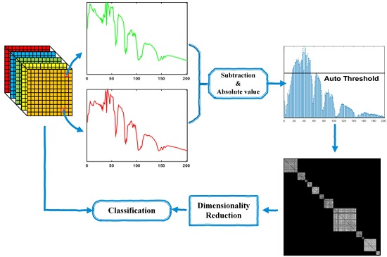
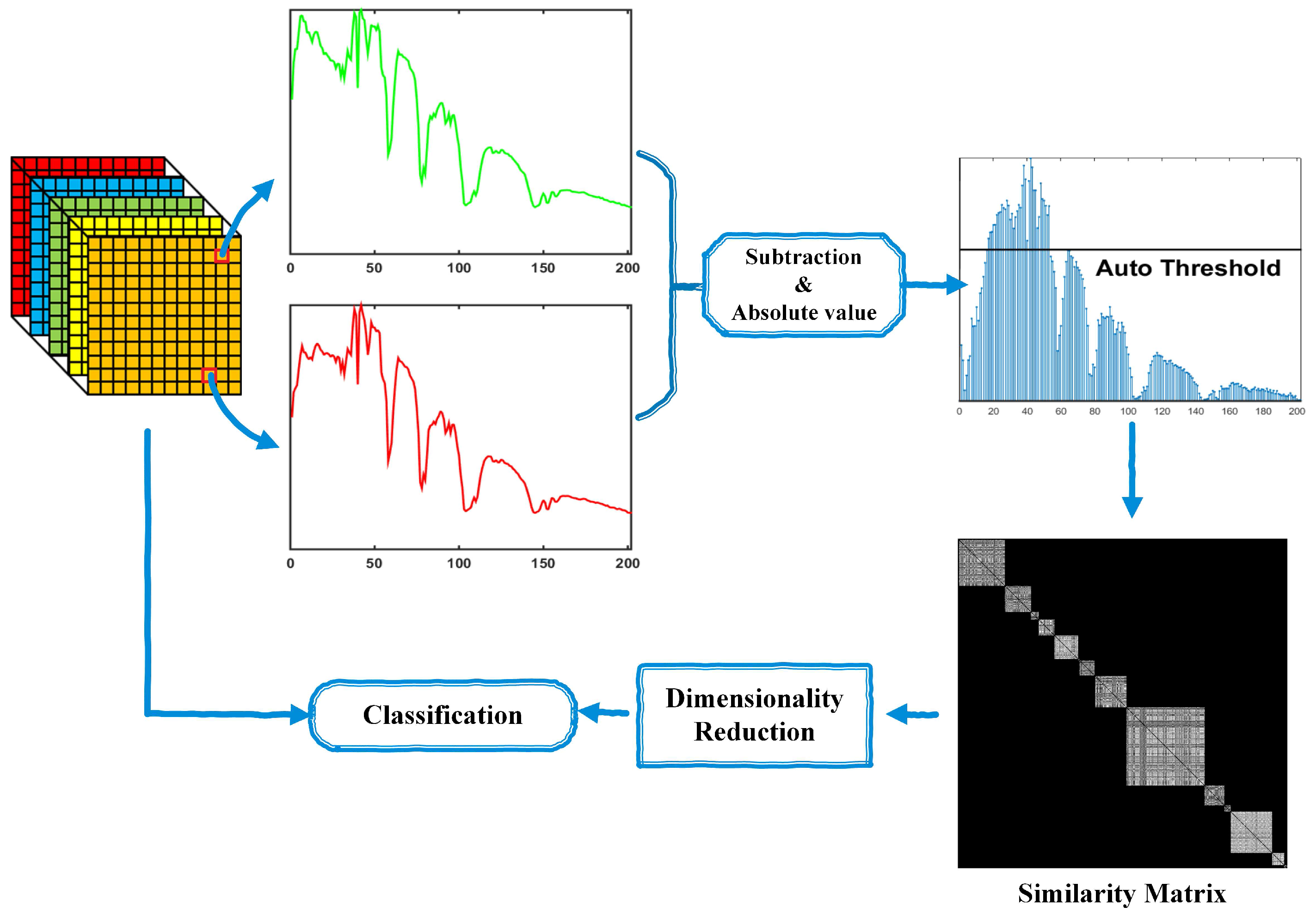
Recently, various graph-based algorithms are demonstrated to be effective for solving dimensionality reduction problems in high-dimensional data [26,27,28,29]. How to construct the similarity graph plays a vital role in these algorithms. The performance of these methods largely hinges on whether the graph can accurately distinguish the similarity and dissimilarity among data points, even when the data contain noise. In this section, two popular approaches to construct affinity graphs are summarized.

The first approach is pairwise distance. In this part, the most popular metric is Euclidean distance with Heat Kernel, typically used in LPP [13], i.e.,

$$\mathrm{sim}({\mathbf{x}}_i,{\mathbf{x}}_j)={\exp }^{\frac{{∥{\mathbf{x}}_i-{\mathbf{x}}_j∥}_2^2}{\tau }},$$

(4)

where $\mathrm{sim}(·)$ represents the similarity function, ${\mathbf{x}}_i$ and ${\mathbf{x}}_j$ denote data points (vector), and parameter $\tau$ denotes the width of the Heat Kernel.

This metric has been applied in various domains such as face recognition [30] and anomaly detection [31]. However, it is generally known that the pairwise distance is very sensitive to the noise and outliers because its measurement just depends on the corresponding two data points. Thus, the algorithms based on the first strategy may fail to manage noise corrupted data.

The other approach for building graphs is the reconstruction coefficients, typically used in SGDA [22]. Sparse representation utilizes a few bases to represent each data point, which is successfully used in data representation. The original formula is expressed as

$$\begin{array}{c}\mathbf{W}=argmin{∥\mathbf{W}∥}_1\hfill \\ \mathrm{s}.\mathrm{t}.\mathbf{X}=\mathbf{XW},diag\left(\mathbf{W}\right)=0,\hfill \end{array}$$

(5)

where $\mathbf{W}$ is the affinity matrix and $∥·∥$ denotes the ${\ell }_1$-norm. Because of the classes of the labeled samples, $\mathbf{W}$ can be written as,

$$\left[\begin{array}{cccc}{\mathbf{W}}^{\left(1\right)}& 0& \cdots & 0\\ 0& {\mathbf{W}}^{\left(2\right)}& \cdots & 0\\ ⋮& ⋮& \ddots & ⋮\\ 0& \cdots & 0& {\mathbf{W}}^{\left(C\right)}\end{array}\right],$$

(6)

where ${\mathbf{W}}^{\left(i\right)}$ is the sparse representation matrix whose size is $M_i\times M_i$ for the samples in the ith class using the $M_i$ samples just belonging to $C_i$.

3. Proposed GDA-SS

In this section, the proposed method, i.e., GDA-SS, is introduced in detail. GDA-SS is motivated by simple spectral operations as illustrated in Figure 1. The training samples are randomly chosen to construct a similarity graph using the proposed spectral similarity measurement; then, graph-embedding dimensionality reduction framework is applied to project the samples into lower dimensional subspace. Because each spectral vector reveals the spectral information in a certain wavelength range, the proposed approach can translate the characteristic into a similarity graph well.

3.1. GDA-SS

Considering ${\mathbf{x}}_i,{\mathbf{x}}_j$ is in the same class as the hyperspectral data, the difference of these two samples can be written as

$${\mathbf{x}}_{sub}=\left|{\mathbf{x}}_i-{\mathbf{x}}_j\right|,$$

(7)

where $\left|·\right|$ denotes the absolute value. It is obvious that the subtraction can reveal the difference between two spectral pixels. After that, the subtraction needs a threshold to constrain the similarity distance. In fact, pixels may be disturbed by a sensor noise to some degree. Thus, in order to take the edge off the noise, a ratio of average subtraction is applied to measure the similarity. That is, the threshold $T_d$ is represented as

$$T_d=\mathrm{avg}\left({\mathbf{x}}_{sub}\right)\times \eta ,$$

(8)

where $\mathrm{avg}(·)$ denotes the average value of elements in ${\mathbf{x}}_{sub}$, and $\eta$ is an adjustment parameter. In experiments, the average value is replaced by that from a set of pair-wise differences in the same class.

When the threshold $T_d$ is confirmed, the similarity can be calculated by comparing ${\mathbf{x}}_{sub}$ with $T_d$. The number of elements whose values are less than $T_d$ is counted. Then, the similarity between ${\mathbf{x}}_i$ and ${\mathbf{x}}_j$ is determined as

$$\mathrm{sim}({\mathbf{x}}_i,{\mathbf{x}}_j)=\frac{\sum ({\mathbf{x}}_{sub}<T_d)}{d},$$

(9)

which is the $ij$th element in matrix $\mathbf{W}$, and d is the number of bands. To make the $\mathbf{W}$ even more sparse, the elements in $\mathbf{W}$ less than another given threshold $T_s$ are set to $zero$. According to the difference in individual classes, separate threshold $T_s^l$ can be set,

$$T_s^l=max\left({\mathbf{W}}^l\right)\times \gamma ,$$

(10)

where ${\mathbf{W}}^l$ denotes pair-wise similarity of samples in the lth class, and $\gamma$ is a sparsity-controlling parameter.

3.2. Analysis on GDA-SS

For a hyperspectral image, spectrum is the important characteristic, which makes the pixel-level classification a reality. However, each pixel may be interfered with by noise (such as some inevitable random noise). In this way, the parameters are very important for adjusting the data-dependent features. The benefit of this proposed approach is that spectral similarity between two pixels is calculated by chosen bands not all the bands, through thresholding the spectral difference. With the chosen bands, trivial spectral variations and additive noise can be alleviated, resulting in better representation of spectral similarity.

In GDA-SS, there are two important parameters, i.e., $\eta$ and $\gamma$, controlling the spectral similarity and sparseness, respectively. We illustrate three-class synthetic data (here, three classes are chosen from the University of Pavia data that will be introduced in Section 4) to demonstrate the sensitivity of these two parameters. The typical support vector machine (SVM) [32,33] is employed to measure the classification accuracy. The signal-to-noise ratio (SNR) of 20 dB and 30 dB Gaussian noise [34] and infinite (here, Inf means that no additional noise is used) is simulated. Figure 2 illustrates the graph matrix learned by GDA-SS with the pre-setting parameters. When the dimensionality is reduced to 25, the best classification accuracies are 98.25%, 99.25%, and 99.50%, respectively, and we obtain corresponding controlling parameters, i.e., $\eta$ and $\gamma$, as shown in Figure 2. Note that when the SNR is smaller, the resulting parameter $\eta$ is larger. This is because too much noise can affect the threshold $T_d$. Under the situation, $\eta$ needs to change for suiting the situation. In general, the higher SNR needs larger $\eta$ because Equation (9) requires a litter higher tolerance. As for parameter $\gamma$, its function (role) is to control the sparseness of graph matrix. Compared to Figure 2a,c, even though the $\gamma$ value is the same, the $\eta$ value is significantly different, which results in the sparsity in Figure 2a being worse than that in Figure 2c. It demonstrates that controlling parameters $\gamma$ and $\eta$ can adaptively tune the sparsity, and when the SNR is larger, the sparsity may be worse.

4. Experimental Results

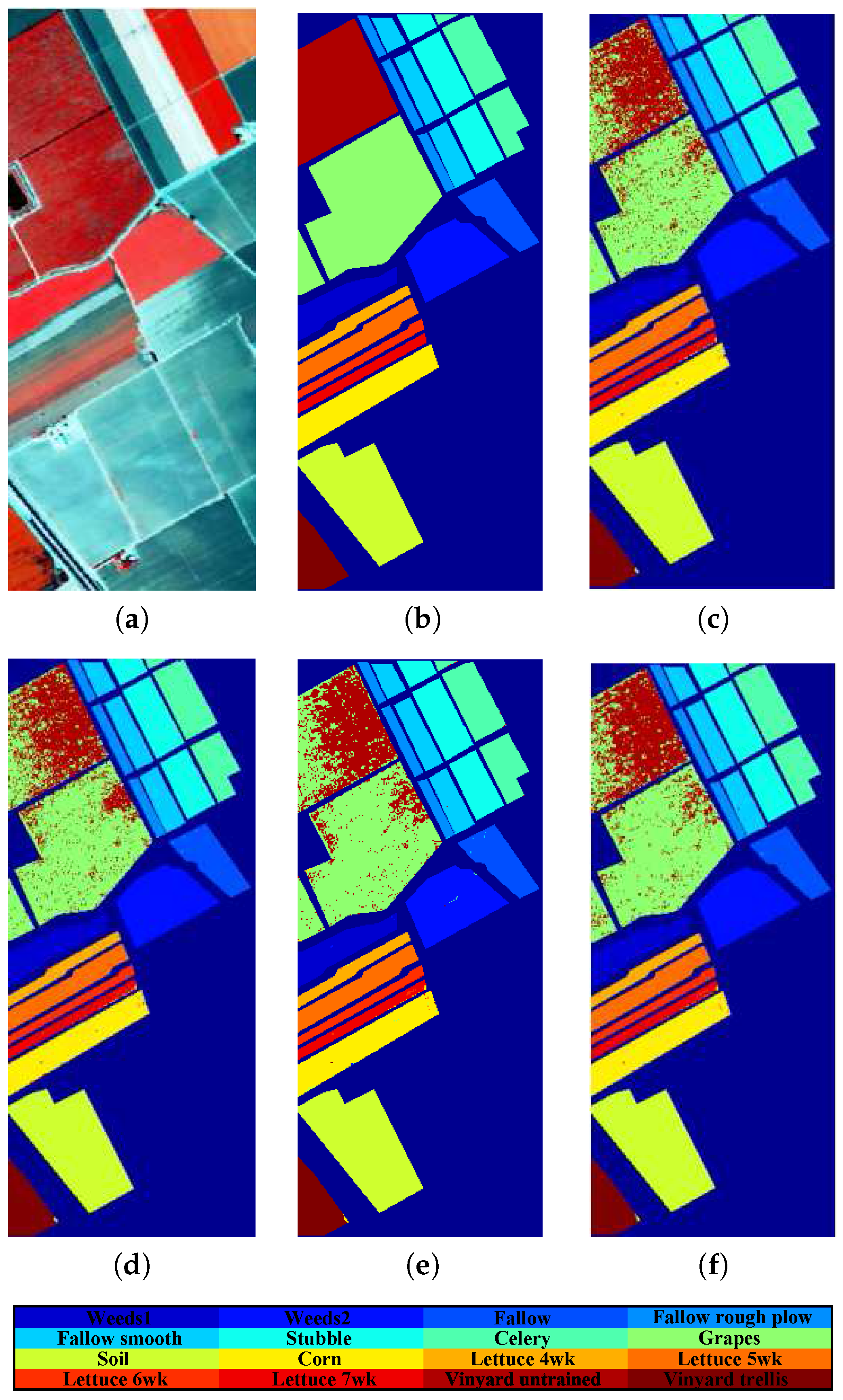
4.1. Hyperspectral Data

In experiments, real hyperspectral data sets have been used to test the proposed method. The first dataset (http://www.ehu.eus/ccwintco/index.php?title=Hyperspectral_Remote_Sensing_Scenes) employed in the experiment was acquired using National Aeronautics and Space Administration’s (NASA) Airborne Visible/Infrared Imaging Spectrometer (AVIRIS) sensor over Salinas Valley, Central Coast of California, in 1998. The image includes $512\times 217$ pixels with a high spatial resolution of 3.7 m and 204 bands after 20 water absorption bands are removed. It mainly contains vegetables, bare soils, and vineyard fields. There are also 16 classes, and the number of training and testing samples are listed in

Table 1. SVM class-specific accuracy (%), overall accuracy (OA) and average accuracy (AA) of different techniques for the Salinas dataset.

	Class	Train	Test	LDA	SLPP	SGDA	GDA-SS
1	Brocoli-green-weeds-1	100	1909	99.75	100	99.63	99.90
2	Brocoli-green-weeds-2	186	3540	99.79	99.97	99.97	99.97
3	Fallow	99	1877	99.75	99.68	99.84	99.79
4	Fallow-rough-plow	70	1324	99.64	99.32	99.09	98.94
5	Fallow-smooth	134	2544	98.54	98.47	98.43	98.43
6	Stubble	198	3761	99.77	99.28	99.31	99.34
7	Celery	179	3400	99.80	99.82	99.71	99.74
8	Grapes-untrained	564	10,707	84.38	86.79	89.33	89.93
9	Soil-vinyard-develop	310	5893	98.19	99.64	99.63	99.78
10	Corn-senesced-green-weeds	164	3114	97.99	96.82	97.11	97.69
11	Lettuce-romaine-4wk	53	1015	98.31	97.04	99.21	98.72
12	Lettuce-romaine-5wk	96	1831	99.74	99.73	99.89	99.89
13	Lettuce-romaine-6wk	46	870	98.69	98.74	98.16	98.51
14	Lettuce-romaine-7wk	54	1016	96.45	95.18	92.52	95.28
15	Vinyard-untrained	363	6905	60.66	63.50	71.06	70.33
16	Vinyard-vertical-trellis	90	1717	99.39	99.20	99.30	99.30
OA				90.85	91.94	93.26	93.40
AA				95.68	95.83	96.39	96.59

, where 5% of the labeled samples in each class are randomly chosen to be training samples and the rest for testing samples.

The second experimental dataset was collected by the Reflective Optics System Imaging Spectrometer (ROSIS) sensor over the city of Pavia, northern Italy. The one is a Pavia University scene, which covers a spatial coverage of $610\times 340$ pixels. The dataset has 103 spectral bands prior to water-band removal with a spectral coverage from 0.43- to 0.86-$\mathsf{\mu }$m and a spatial resolution of 1.3 m. Approximately 42,776 labeled pixels with nine classes are from the ground truth map. In this dataset, 8% of the labeled samples are randomly selected for training and the rest for testing. More detailed information of the number of training and testing samples are summarized in

Table 2. SVM class-specific accuracy (%), overall accuracy (OA) and average accuracy (AA) of different techniques for the University of Pavia dataset.

	Class	Train	Test	LDA	SLPP	SGDA	GDA-SS
1	Asphalt	530	6101	93.39	91.51	92.17	95.33
2	Meadows	1492	17,157	96.36	95.68	96.96	97.65
3	Gravel	168	1931	58.74	64.16	62.40	70.53
4	Trees	245	2819	90.86	90.49	94.08	93.33
5	Painted Metal Sheets	108	1237	99.48	99.60	99.76	99.84
6	Bare Soil	402	4627	78.99	76.92	88.48	92.33
7	Bitumen	106	1224	75.41	66.26	76.88	79.33
8	Self-Blocking Bricks	295	3387	86.11	82.70	87.95	91.23
9	Shadows	76	871	99.37	99.77	95.14	99.89
OA				90.51	89.09	92.56	94.02
AA				86.52	85.23	88.73	91.05

.

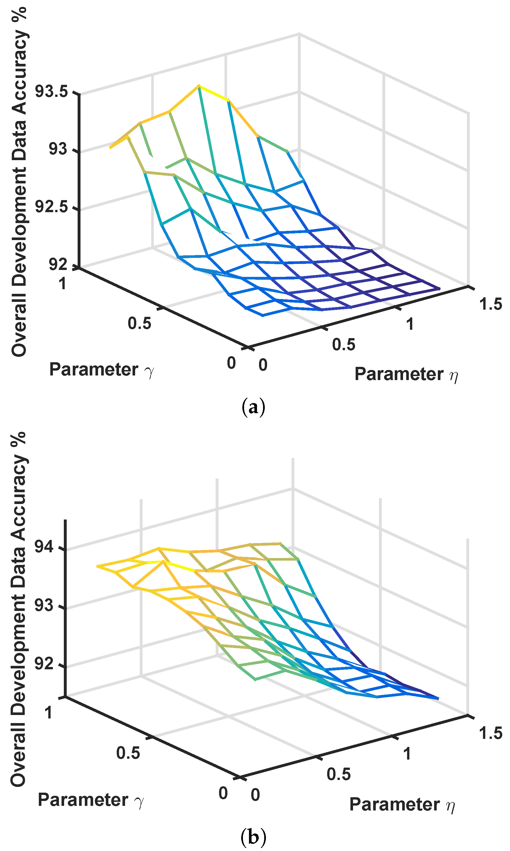
4.2. Parameter Tuning

The classical SVM is employed to validate the aforementioned dimensionality-reduction methods, including LDA, SLLP, SGDA, and GDA-SS. A fivefold cross-validation strategy is employed for tuning parameters in classification tasks.

Figure 3 illustrates the sensitivity of the proposed GDA-SS as functions of two parameters (i.e., $\eta$ and $\gamma$) in the objective functions (e.g., Equations (8) and (10)). In the experiment, $\eta$ is chosen from 0.1 to 1.3, where the interval is 0.2 and $\gamma$ is chosen from 0 to 0.9, where the interval is 0.1. Noted that the parameter $\eta$ can be chosen as greater than 1 due to considering that the data may be pure. However, $\eta$ cannot be greater; if so, the measurement may contain more errors. It is obvious that when the parameter $\gamma$ is chosen as 0, the similarity matrix is theoretically no longer “sparse”. Optimal $\eta$ and $\gamma$ are determined for GDA-SS from the results in Figure 3. For example, according to the validation classification accuracy, the best $\eta$ of GDA-SS is 0.7 and the one of $\gamma$ is 0.9 for the Salinas data; and for the University of Pavia dataset, $\eta$ is set to 0.3 and $\gamma$ is set to 0.7. It is worth mentioning that a nonzero value of $\gamma$ verifies that the “sparseness” ratio can have an impact on the dimensionality reduction process.

To demonstrate the effect of the dimensionality of the projected subspace on the performance of the proposed methods, Figure 4 illustrates the classification accuracy as a function of the reduced-dimensionality K for LDA, SLPP, SGDA and GDA-SS. SLPP is chosen for comparison because all of the methods are supervised. It is obvious that the performance tends to be stable when the dimensionality is larger than a certain value. For the Salinas dataset, a reduced dimension of 25 appears to be sufficient, whereas approximately 10 is enough for the University of Pavia dataset. Based on the curves in Figure 4, for a low dimensionality, classification accuracy is often not high, while that of GDA-SS is always better than LDA, SLPP, and SGDA. For the Salinas data, when the reduced dimensionality is more than 25, the performance of SGDA tends to decline, whereas GDA-SS tends to be stable. Furthermore, when the reduced dimensionality is smaller than 7, the proposed GDA-SS is superior to SGDA. Thus, this result further confirms that the proposed strategy is able to find a transform that can effectively reduce the dimensionality while enhancing class separability.

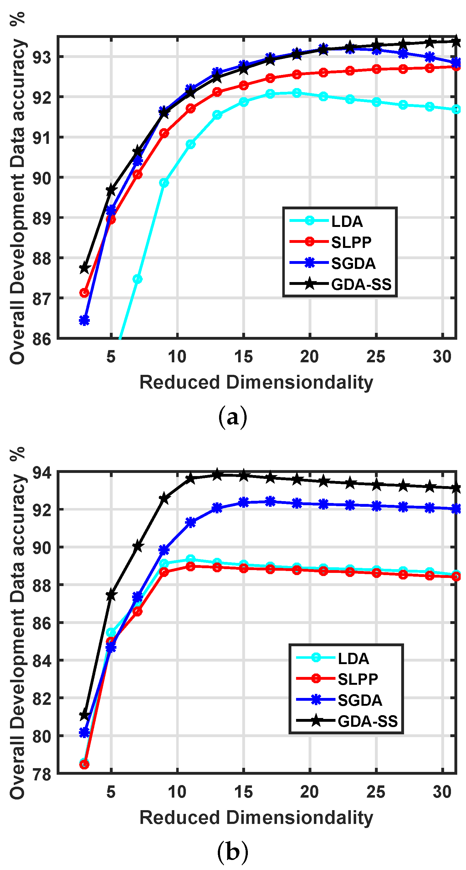
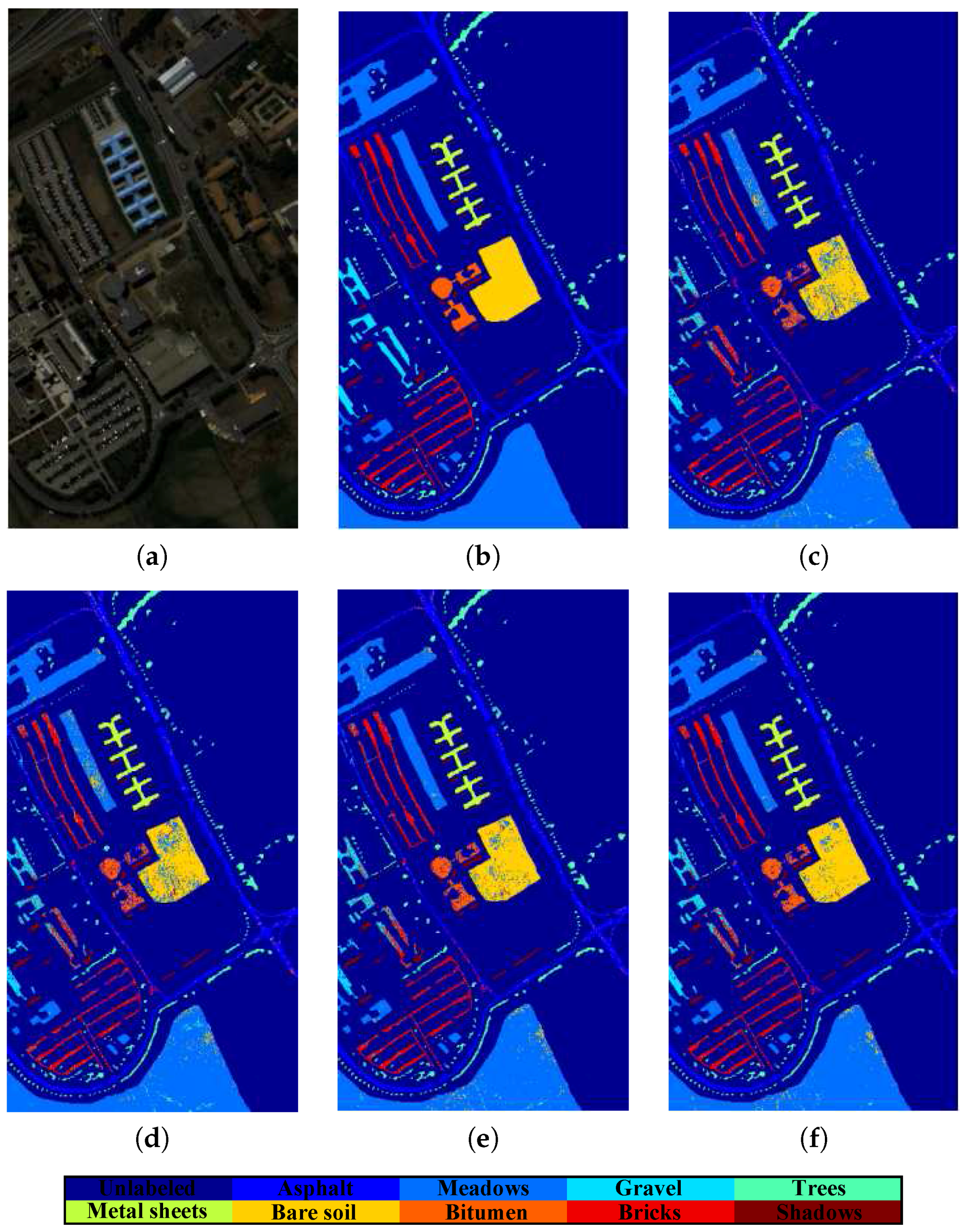
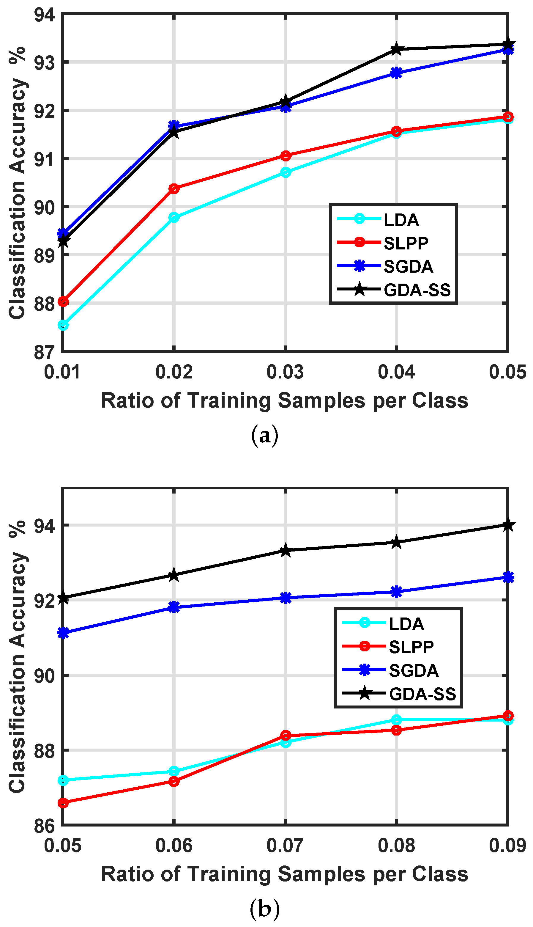
4.3. Classification Performance

In order to further evaluate the performance of GDA-SS, we compare the proposed method with the traditional LDA, SLPP and the state-of-the-art SGDA in each optimal dimensionality, respectively. Table 1 and Table 2 list the class-specific accuracy, overall accuracy and average accuracy for the experimental datasets. From the results of each method, the traditional LDA and SLPP are usually a little worse than state-of-the-art SGDA since ${\ell }_1$-norm can better capture the data structure. However, the proposed GDA-SS with sparse-controlling parameter $\gamma$ can be better than SGDA. For example, in Table 2, GDA-SS (i.e., 94.02%) yields over 1% higher accuracy than SGDA (i.e., 92.56%). Meanwhile, the $\gamma$, which is set to 0.7, verifies that the similarity is “sparse”.

Figure 5 and Figure 6 further illustrate the thematic maps. We produce ground-cover maps of the entire image scene for these images (including unlabeled pixels). However, to facilitate easy comparison between methods, only areas for which we have ground truth are shown in these maps. These maps are consistent with the results listed in Table 1 and Table 2, respectively. Some areas in the classification maps produced by GDA-SS are obviously less noisy than these of SGDA, e.g., the regions of Bare soil and Bricks in Figure 6. Figure 7 further shows the comparisons between the proposed GDA-SS and these traditional methods with different numbers of training samples. For the Salinas data, the training size is changed from 0.01 to 0.05 (note that 0.05 is the ratio of number of training samples to the total labeled data). It is obvious that the classification performance of the proposed GDA-SS is competitive to the state-of-the-art SGDA. For the University of Pavia data, the improvement always keeps as 1%.

In

Table 3. Statistical significance from the Standardized McNemar’s Test about the difference between methods.

Salinas Z/Significant?	University of Pavia Z/Significant?
GDA-SS vs. SGDA
4.91/yes	12.33/yes
GDA-SS vs. SLPP
16.87/yes	35.17/yes
GDA-SS vs. LDA
18.56/yes	33.55/yes

, the standardized McNemar’s test [35] is employed to testify the improvement. The Z values of McNemar’s test larger than 2.58 mean that two classification results are statistically different at a 99% confidence level. According to our experimental results, the Z values between GDA-SS and SGDA, SLPP, and LDA are always larger than 2.58, which confirms that the proposed GDA-SS is able to highly discriminate between the different classes. For example, even though the classification accuracy of SGDA and GDA-SS is close for the Salinas data, the Z value between these two methods is 4.91, which indicates that the improvement is significant.

4.4. More Robustness Test of GDA-SS

Additional discussion on graph construction with distance similarity is presented. For graphbased dimensionality reduction methods, the most important part is to construct an informative graph. Here, several distance-similarity approaches, including cosine, Jaccard, and correlation coefficient, are employed to evaluate the spectral similarity measurement under the framework of GDA-SS in

Table 4. Classification evaluation on graph construction with different distance-similarity metrics.

Distance Datasets	Salinas	Univesity of Pavia
Proposed	93.40	94.02
Cosine	91.92	91.13
Jaccard	92.01	90.83
Correlation	91.91	91.18

. Compared with the proposed one, these traditional distance-similarity metrics provide worse performance, although all the accuracy values are higher than 90%. The experiment verifies that the proposed method is more effective in measuring spectral similarity.

Furthermore, considering that hyperspectral spectra contain noise, aforementioned dimension reduction methods are compared after noise filtering techniques are applied. Here, two commonly-used filtering methods (i.e., local average filter and wavelet de-noising) are employed as preprocesses for these experimental datasets. In

Table 5. Classification results after applying noise filtering techniques.

	Salinas			University of Pavia
	No Filter	Average Filter	Wavelet De-Noising	No Filter	Average Filter	Wavelet De-Noising
GDA-SS	93.40	93.41	93.40	94.02	94.08	94.05
SGDA	93.26	93.46	93.41	92.56	92.93	92.76
SLPP	91.94	91.95	91.74	89.09	89.08	89.02
LDA	90.85	92.24	92.24	90.51	89.51	89.59

, it shows that denoising has no obvious impact on these algorithms for the University of Pavia dataset. However for the Salinas dataset, the accuracies of SGDA and LDA are slightly improved, and GDA-SS still maintains a high accuracy, which demonstrates that GDA-SS is less sensitive to noise.

5. Conclusions

In this paper, a graph-based discriminant analysis via spectral similarity (GDA-SS) framework was proposed. In this method, spectral similarity using chosen band information was incorporated into the affinity matrix, and similarity measurement is less affected by trivial spectral variation and noise. The controlling parameters $\eta$ and $\gamma$ were validated to be effective for constructing affinity matrix, from the perspectives of spectral similarity and sparseness. The results of real hyperspectral images demonstrated that the proposed GDA-SS is superior to the traditional LDA, SLPP, and the state-of-the-art SGDA, even under small-sample-size situations. Moreover, the computational cost of GDA-SS is much lower than SGDA because only simple arithmetic operations are involved during graph construction. This makes it potentially more suitable to solve big data problems.

References

1. Prasad, S.; Li, W.; Fowler, J.E.; Bruce, L.M. Information Fusion in the Redundant-Wavelet-Transform Domain for Noise-Robust Hyperspectral Classification. IEEE Trans. Geosci. Remote Sens. 2012, 50, 3474–3486. [Google Scholar]
2. Du, B.; Zhang, L.; Zhang, L.; Chen, T.; Wu, K. A Discriminative Manifold Learning Based Dimension Reduction Method for Hyperspectral Classification. Int. J. Fuzzy Syst. 2012, 14, 272–277. [Google Scholar]
3. Gao, L.; Li, J.; Khodadadzadeha, M.; Plaza, A.; Zhang, B.; He, Z.; Yan, H. Subspace-Based Support Vector Machines for Hyperspectral Image Classification. IEEE Geosci. Remote Sens. Lett. 2015, 12, 349–353. [Google Scholar]
4. Li, W.; Tramel, E.W.; Prasad, S.; Fowler, J.E. Nearest Regularized Subspace for Hyperspectral Classification. IEEE Trans. Geosci. Remote Sens. 2014, 52, 477–489. [Google Scholar] [CrossRef]
5. Li, W.; Chen, C.; Su, H.; Du, Q. Local Binary Patterns and Extreme Learning Machine for Hyperspectral Imagery Classification. IEEE Trans. Geosci. Remote Sens. 2015, 53, 3681–3693. [Google Scholar] [CrossRef]
6. Gu, Y.; Liu, T.; Jia, X.; Benediktsson, J.A.; Chanussot, J. Nonlinear Multiple Kernel Learning with Multiple-Structure-Element Extended Morphological Profiles for Hyperspectral Image Classification. IEEE Trans. Geosci. Remote Sens. 2016, 54, 3235–3247. [Google Scholar] [CrossRef]
7. Prasad, S.; Bruce, L.M. Limitations of Principal Component Analysis for Hyperspectral Target Recognition. IEEE Geosci. Remote Sens. Lett. 2008, 5, 625–629. [Google Scholar] [CrossRef]
8. Li, W.; Prasad, S.; Fowler, J.E.; Bruce, L.M. Locality-Preserving Dimensionality Reduction and Classification for Hyperspectral Image Analysis. IEEE Trans. Geosci. Remote Sens. 2012, 50, 1185–1198. [Google Scholar] [CrossRef]
9. Li, W.; Prasad, S.; Fowler, J.E. Hyperspectral Image Classification Using Gaussian Mixture Model and Markov Random Field. IEEE Geosci. Remote Sens. Lett. 2014, 11, 153–157. [Google Scholar] [CrossRef]
10. Yan, S.; Xu, D.; Zhang, B.; Zhang, H.J.; Yang, Q.; Lin, S. Graph Embedding and Extensions: A General Framework for Dimensionality Reduction. IEEE Trans. Pattern Anal. Mach. Intell. 2007, 29, 40–51. [Google Scholar] [CrossRef] [PubMed]
11. Roweis, S.T.; Saul, L.K. Nonlinear Dimensionality Reduction by Locally Linear Embedding. Science 2000, 290, 2323–2326. [Google Scholar] [CrossRef] [PubMed]
12. Belkin, M.; Niyogi, P. Laplacian eigenmaps and spectral techniques for embedding and clustering. In Proceedings of the Neural Information Processing Systems: Natural and Synthetic, Vancouver, BC, Canada, 3–8 December 2001; Volume 14, pp. 585–591. [Google Scholar]
13. He, X.; Niyogi, P. Locality Preserving Projections. In Advances in Neural Information Processing System; Thrun, S., Saul, L., Schölkopf, B., Eds.; MIT Press: Cambridge, MA, USA, 2004. [Google Scholar]
14. Zhai, Y.; Zhang, L.; Wang, N.; Guo, Y.; Cen, Y.; Wu, T.; Tong, Q. A Modified Locality Preserving Projection Approach for Hyperspectral Image Classification. IEEE Geosci. Remote Sens. Lett. 2016, 13, 1059–1063. [Google Scholar] [CrossRef]
15. Yang, J.; Zhang, D.; Yang, J.; Niu, B. Globally maximizing, locally minimizing: unsupervised discriminant projection with applications to face and palm biometrics. IEEE Trans. Pattern Anal. Mach. Intell. 2007, 29, 650–664. [Google Scholar] [CrossRef] [PubMed]
16. Cai, H.; Mikolajczyk, K.; Matas, J. Learning linear discriminant projections for dimensionality reduction of image descriptors. IEEE Trans. Pattern Anal. Mach. Intell. 2011, 33, 338–352. [Google Scholar] [PubMed]
17. Qiao, L.; Chen, S.; Tan, X. Sparsity Preserving Projections with Applications to Face Recognition. Pattern Recognit. 2010, 43, 331–341. [Google Scholar]
18. Kokiopoulou, E.; Saad, Y. Enhanced graph-based dimensionality reduction with repulsion Laplaceans. Pattern Recognit. 2009, 42, 2392–2402. [Google Scholar] [CrossRef]
19. Zhang, L.; Qiao, L.; Chen, S. Graph-optimized locality preserving projections. Pattern Recognit. 2010, 43, 1993–2002. [Google Scholar] [CrossRef]
20. Zhang, L.; Chen, S.; Qiao, L. Graph optimization for dimensionality reduction with sparsity constraints. Pattern Recognit. 2012, 45, 1205–1210. [Google Scholar] [CrossRef]
21. Peng, X.; Zhang, L.; Yi, Z.; Tan, K.K. Learning Locality-Constrained Collaborative Representation for Robust Face Recognition. Pattern Recognit. 2014, 47, 2794–2806. [Google Scholar] [CrossRef]
22. Ly, N.; Du, Q.; Fowler, J.E. Sparse Graph-Based Discriminant Analysis for Hyperspectral Imagery. IEEE Trans. Geosci. Remote Sens. 2014, 52, 3872–3884. [Google Scholar]
23. Ly, N.; Du, Q.; Fowler, J.E. Collaborative Graph-Based Discriminant Analysis for Hyperspectral Imagery. IEEE J. Sel. Top. Appl. Earth Obs. Remote Sens. 2014, 7, 2688–2696. [Google Scholar]
24. Chen, P.; Jiao, L.; Liu, F.; Zhao, J.; Zhao, Z.; Liu, S. Semi-supervised double sparse graphs based discriminant analysis for dimensionality reduction. Pattern Recognit. 2017, 61, 361–378. [Google Scholar] [CrossRef]
25. Cheng, B.; Yang, J.; Yan, S.; Fu, Y.; Huang, T.S. Learning With 1-Graph for Image Analysis. IEEE Trans. Image Process. 2010, 19, 858–866. [Google Scholar] [CrossRef] [PubMed]
26. He, W.; Zhang, H.; Zhang, L.; Philips, W.; Liao, W. Weighted Sparse Graph Based Dimensionality Reduction for Hyperspectral Images. IEEE Geosci. Remote Sens. Lett. 2016, 13, 686–690. [Google Scholar] [CrossRef]
27. Li, W.; Du, Q. Laplacian Regularized Collaborative Graph for Discriminant Analysis of Hyperspectral Imagery. IEEE Trans. Geosci. Remote Sens. 2016, 54, 7066–7076. [Google Scholar] [CrossRef]
28. Tan, K.; Zhou, S.; Du, Q. Semi-supervised Discriminant Analysis for Hyperspectral Imagery with Block-Sparse Graph. IEEE Geosci. Remote Sens. Lett. 2015, 12, 1765–1769. [Google Scholar] [CrossRef]
29. Li, W.; Liu, J.; Du, Q. Sparse and Low-Rank Graph for Discriminant analysis of Hyperspectral Imagery. IEEE Trans. Geosci. Remote Sens. 2016, 54, 4094–4105. [Google Scholar] [CrossRef]
30. He, X.; Yan, S.; Hu, Y.; Niyogi, P.; Zhang, H.J. Face recognition using Laplacianfaces. IEEE Trans. Pattern Anal. Mach. Intell. 2005, 27, 328–340. [Google Scholar] [PubMed]
31. Zhao, R.; Du, B.; Zhang, L. A robust nonlinear hyperspectral anomaly detection approach. IEEE J. Sel. Top. Appl. Earth Obs. Remote Sens. 2014, 7, 1227–1234. [Google Scholar] [CrossRef]
32. Platt, J. Advances in Large Margin Classifiers. In Probabilistic Outputs for Support Vector Machines and Comparison to Regularized Likelihood Methods; Smola, A., Ed.; MIT Press: Cambridge, MA, USA, 1999. [Google Scholar]
33. Li, C.H.; Kuo, B.C.; Lin, C.T.; Huang, C.S. A Spatial-Contextual Support Vector Machine for Remotely Sensed Image Classification. IEEE Trans. Geosci. Remote Sens. 2012, 50, 784–799. [Google Scholar] [CrossRef]
34. Chen, G.; Qian, S.E. Denoising of Hyperspectral Imagery Using Principal Component Analysis and Wavelet Shrinkage. IEEE Trans. Geosci. Remote Sens. 2011, 49, 973–980. [Google Scholar] [CrossRef]
35. Villa, A.; Benediktsson, J.A.; Chanussot, J.; Jutten, C. Hyperspectral image classification with independent component discriminant analysis. IEEE Trans. Geosci. Remote Sens. 2011, 49, 4865–4876. [Google Scholar] [CrossRef]
Figure 1. The flowchart and the motivation of the proposed GDA-SS.
Remotesensing 09 00323 g001
Figure 2. Visualization of various graph weights: (a) η = 0.9, γ = 0.8; (b) η = 0.7, γ = 0.9; and (c) η = 0.3, γ = 0.8.
Remotesensing 09 00323 g002
Figure 3. Parameter tuning of η and γ for the proposed GDA-SS using two experimental datasets. (a) Salinas; (b) Pavia University.
Remotesensing 09 00323 g003
Figure 4. Classification accuracy versus reduced-dimensionality K for methods using the experimental datasets. (a) Salinas; (b) Pavia University.
Remotesensing 09 00323 g004
Figure 5. Thematic maps resulting from classification for the Salinas dataset with 16 classes. (a) pseudo-color image; (b) ground truth map; (c) LDA: 90.85%; (d) SLPP: 91.94%; (e) SGDA: 93.26%; (f) GDA-SS: 93.40%.
Remotesensing 09 00323 g005
Figure 6. Thematic maps resulting from classification for the University of Pavia dataset with nine classes. (a) pseudo-color image; (b) ground truth map; (c) LDA: 90.51%; (d) SLPP: 89.09%; (e) SGDA: 92.56%; (f) GDA-SS: 94.02%.
Remotesensing 09 00323 g006
Figure 7. Classification performance of methods with different numbers of training sample sizes using the experimental datasets. (a) Salinas; (b) Pavia University.
Remotesensing 09 00323 g007