
Initial Radiometric Characteristics of KOMPSAT-3A Multispectral Imagery Using the 6S Radiative Transfer Model, Well-Known Radiometric Tarps, and MFRSR Measurements


Abstract
:
1. Introduction
2. Materials and Methods
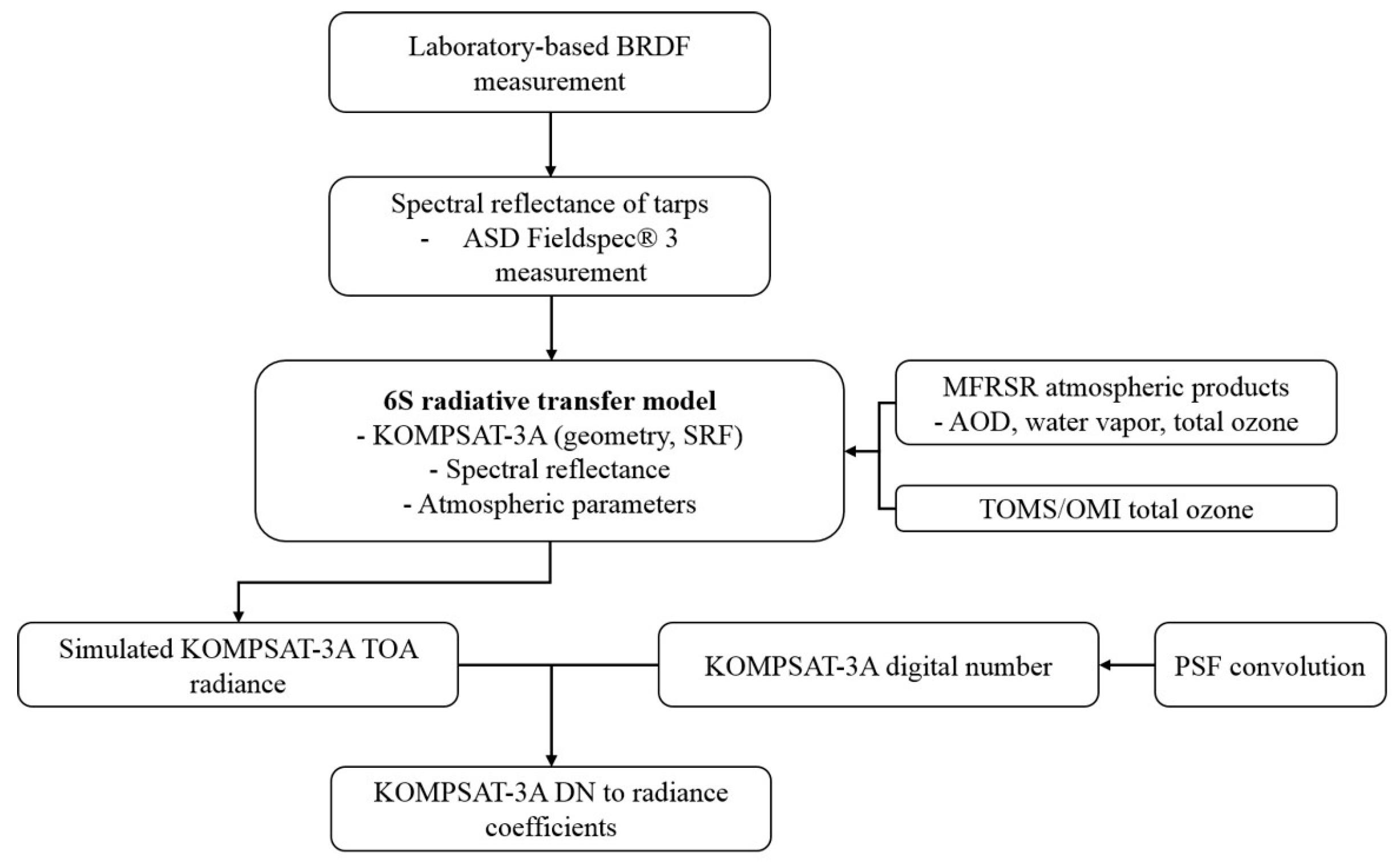
2.1. Schema of Vicarious Calibration Algorithm for KOMPSAT-3A Using 6S Radiative Transfer Model
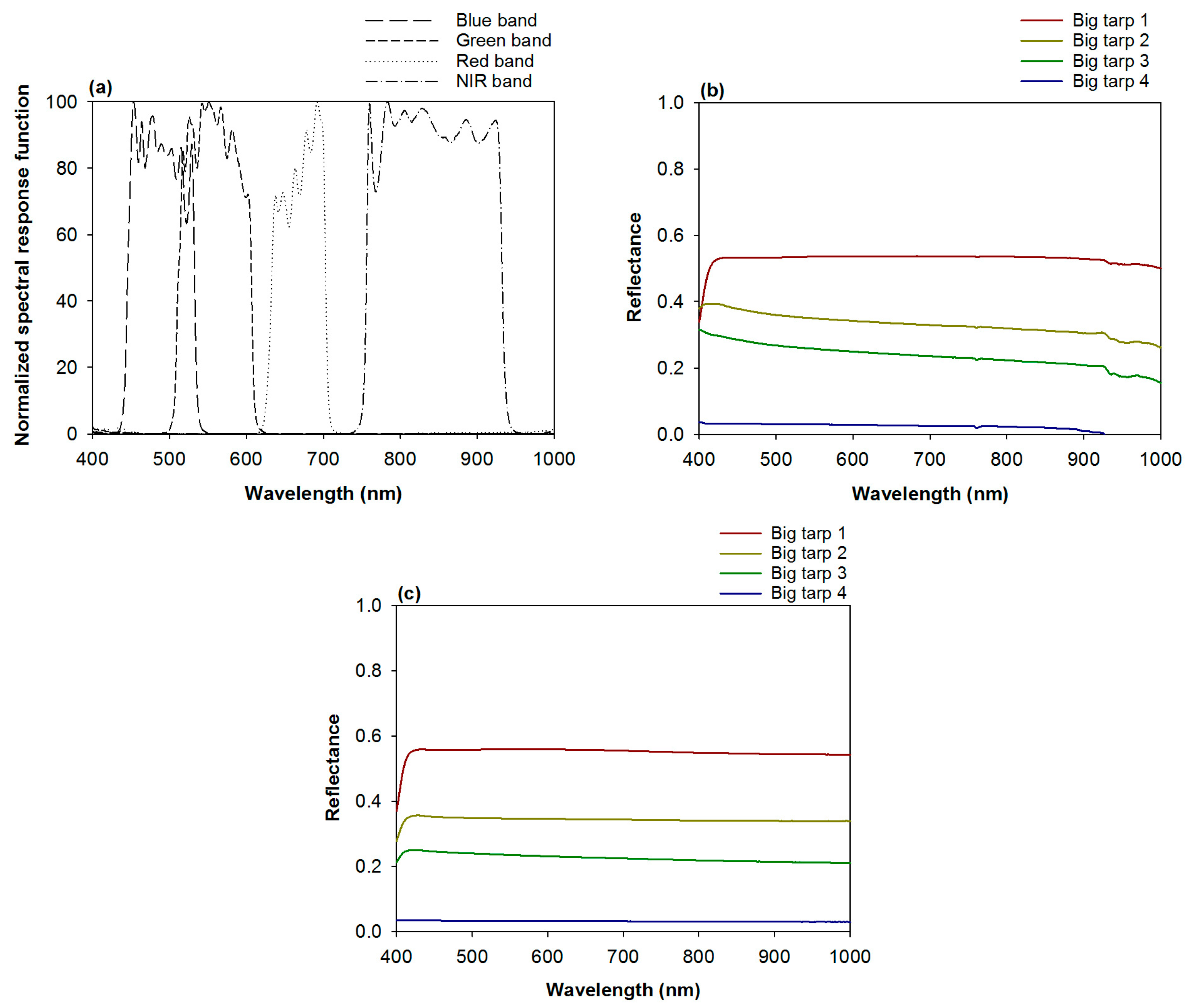
2.2. ASD FieldSpec® 3 Measurements of the Hyperspectral Reflectance of Tarps
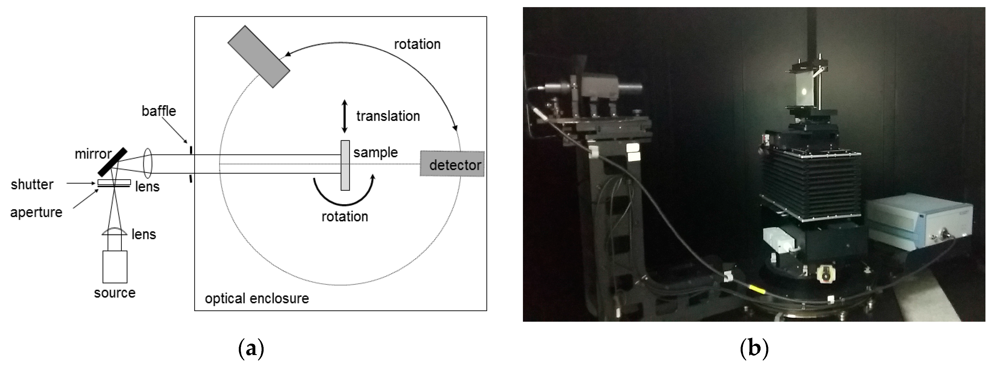
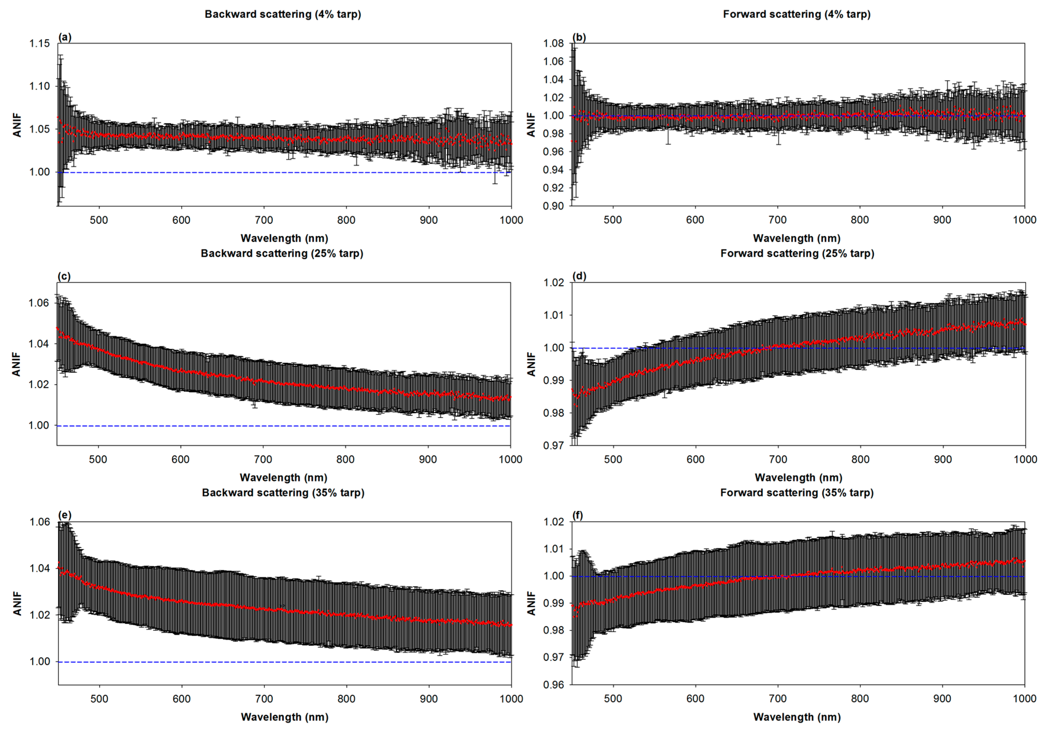
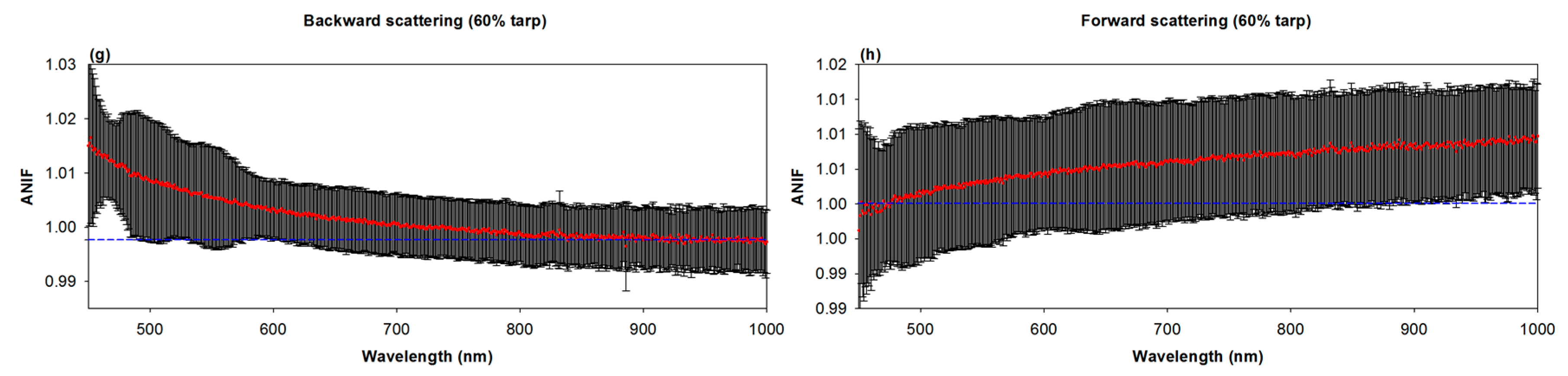
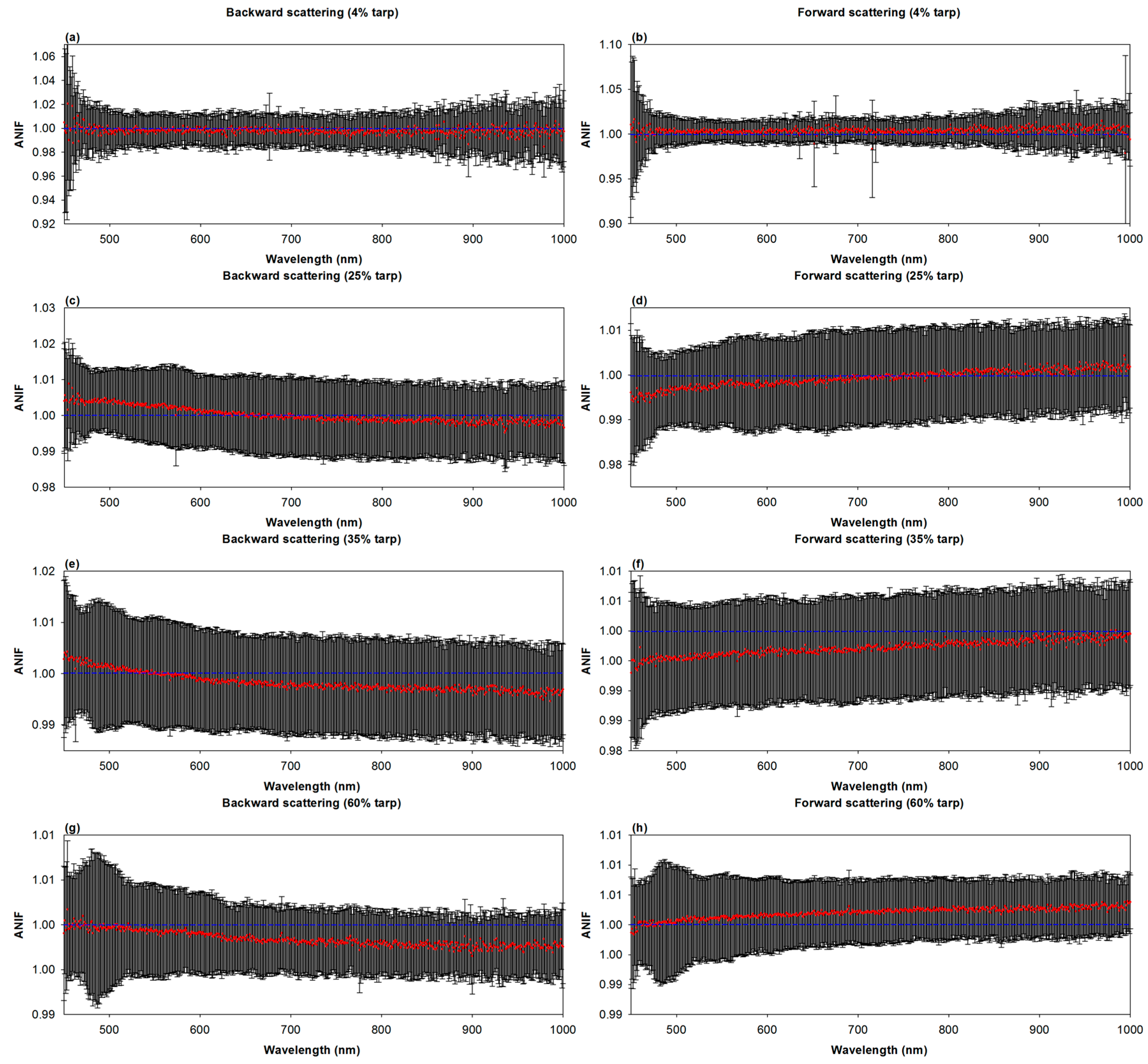
2.3. Laboratory-Based BRDF Measurements of Radiometric Tarps
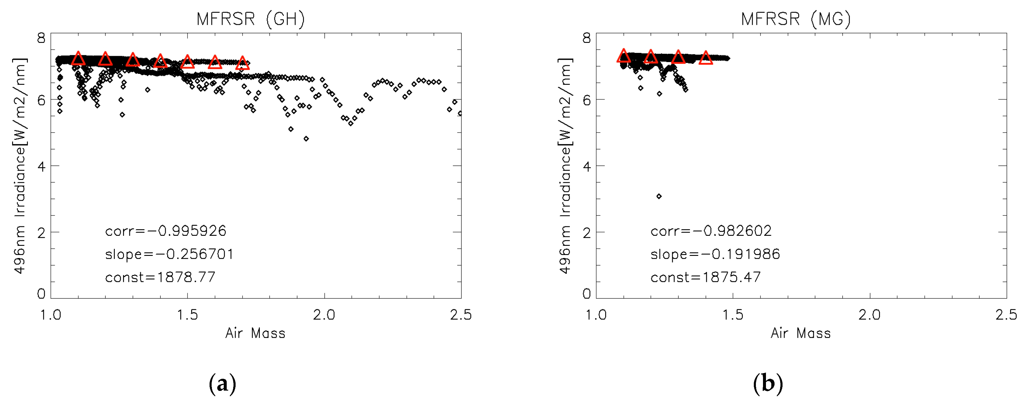
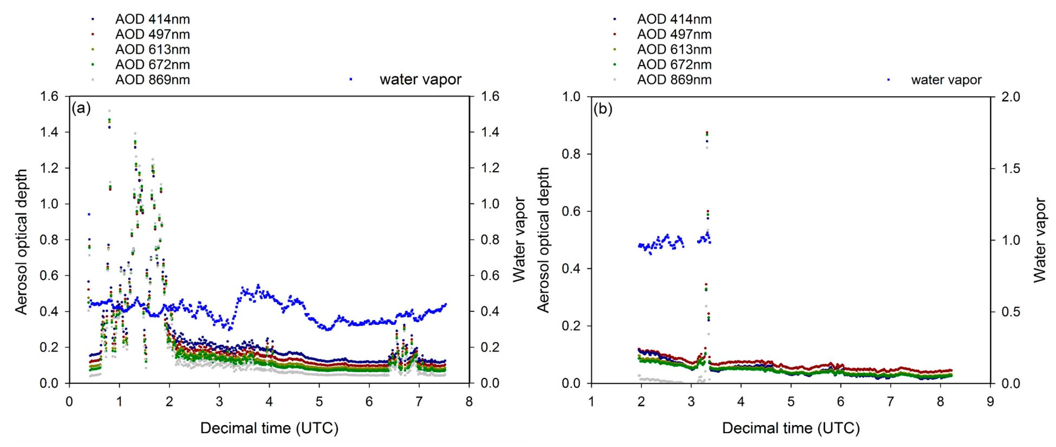
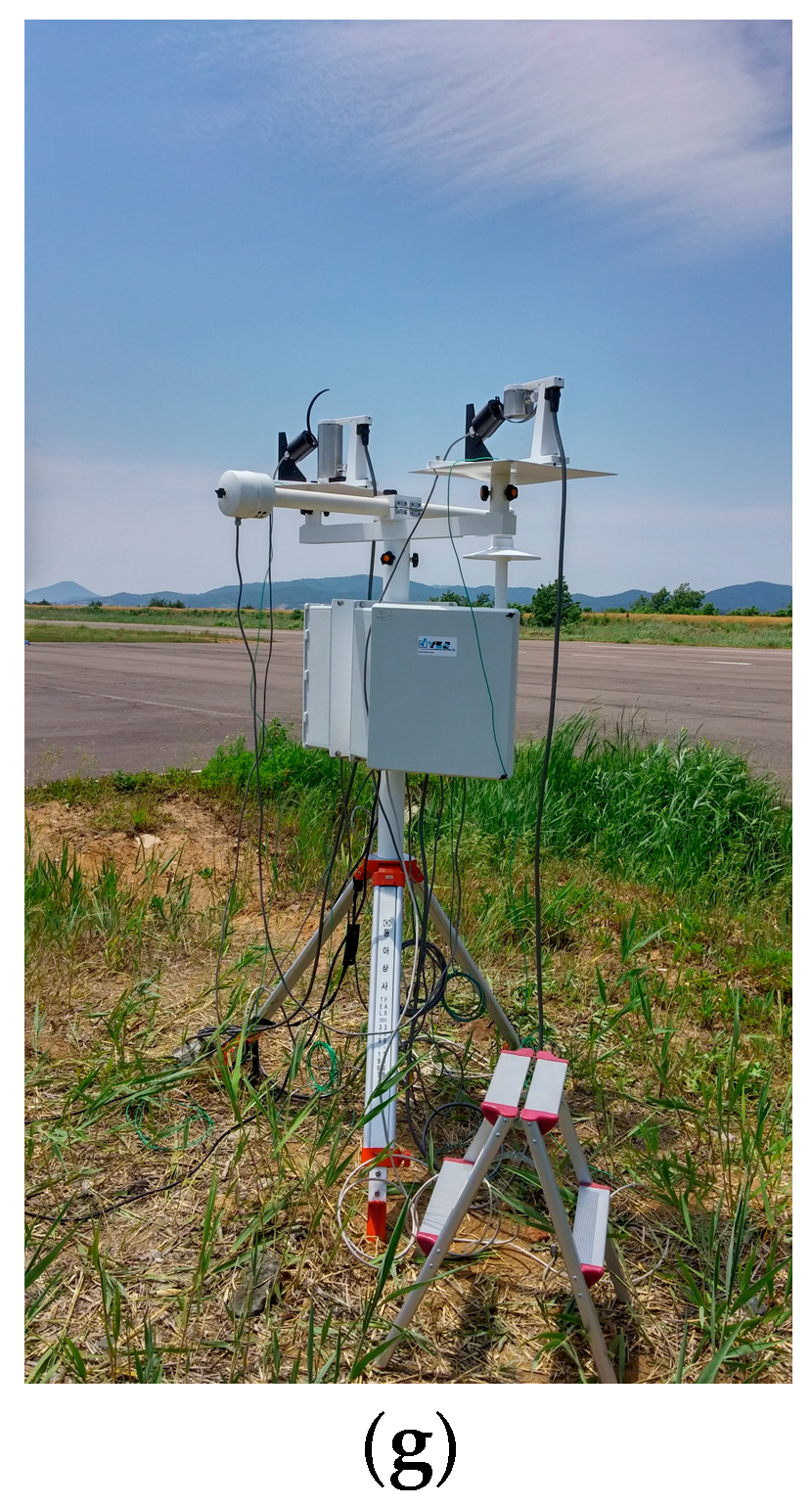
2.4. Atmospheric Conditions Using MFRSR for AOD and Column Water Vapor
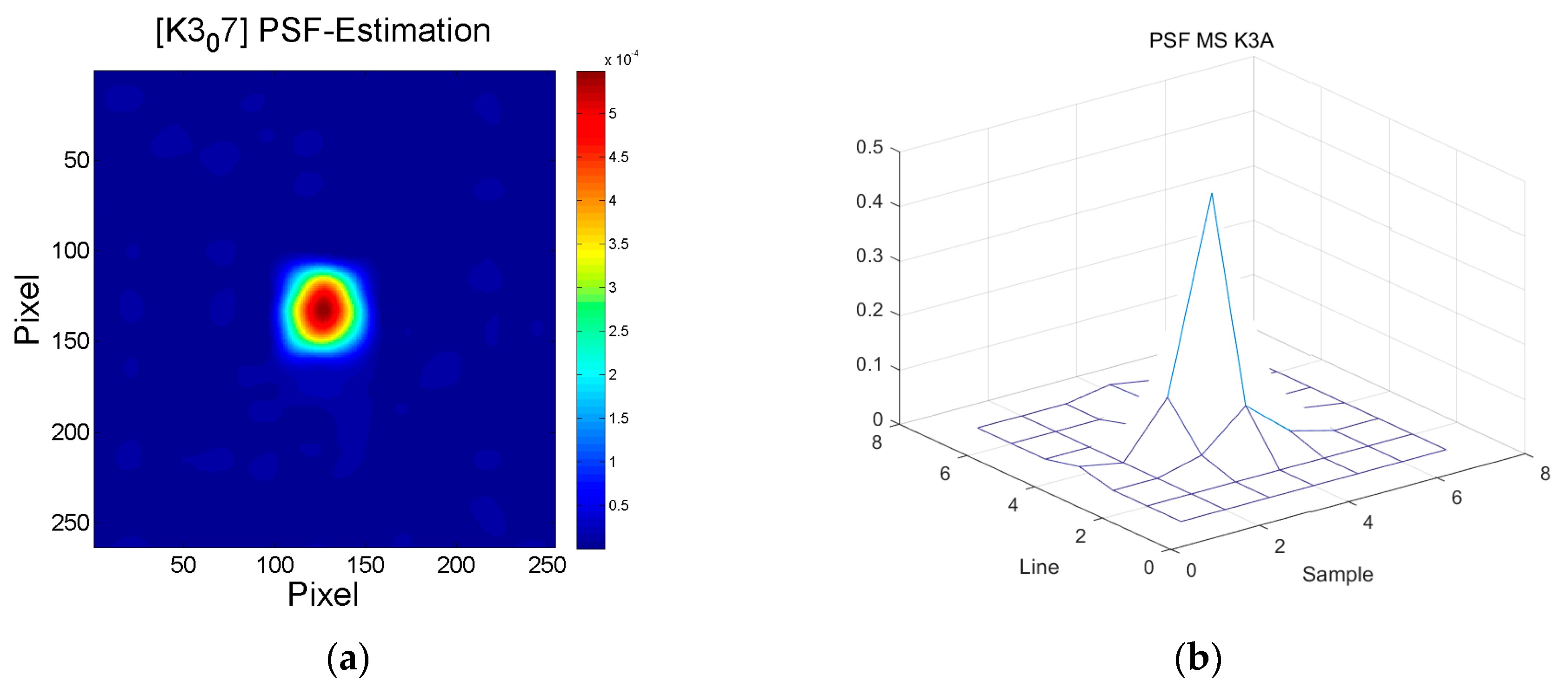
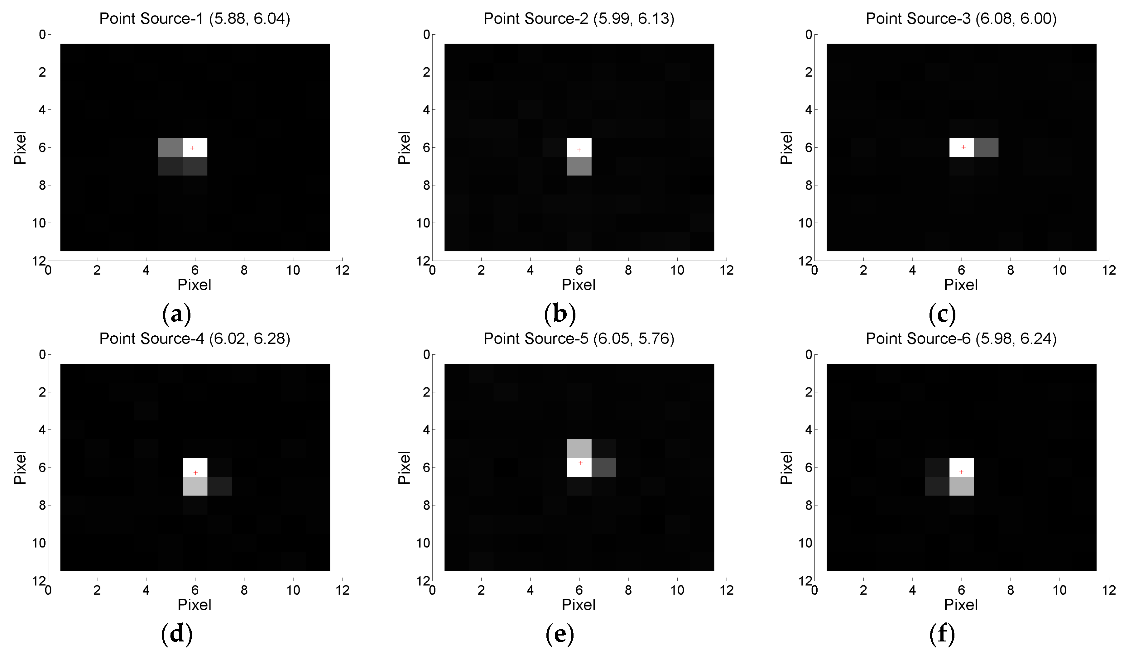
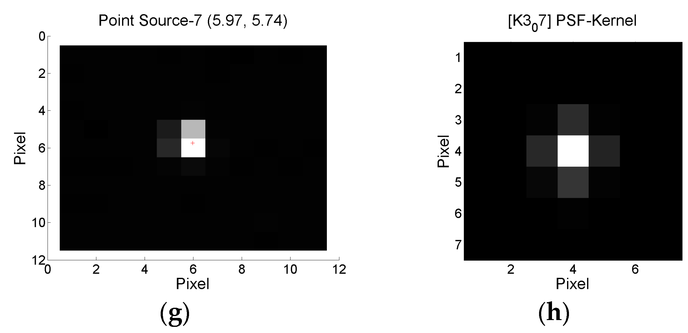
2.5. Retrieval of PSF with KOMPSAT-3A MS Bands by Observing Stars
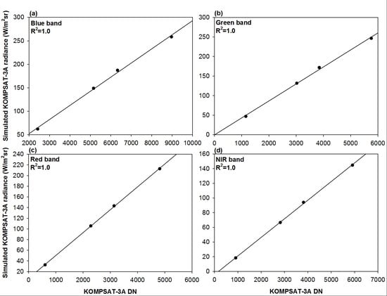
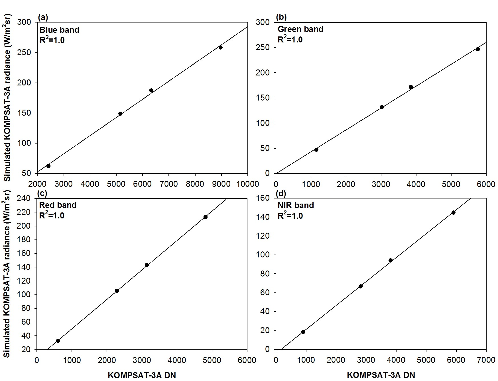
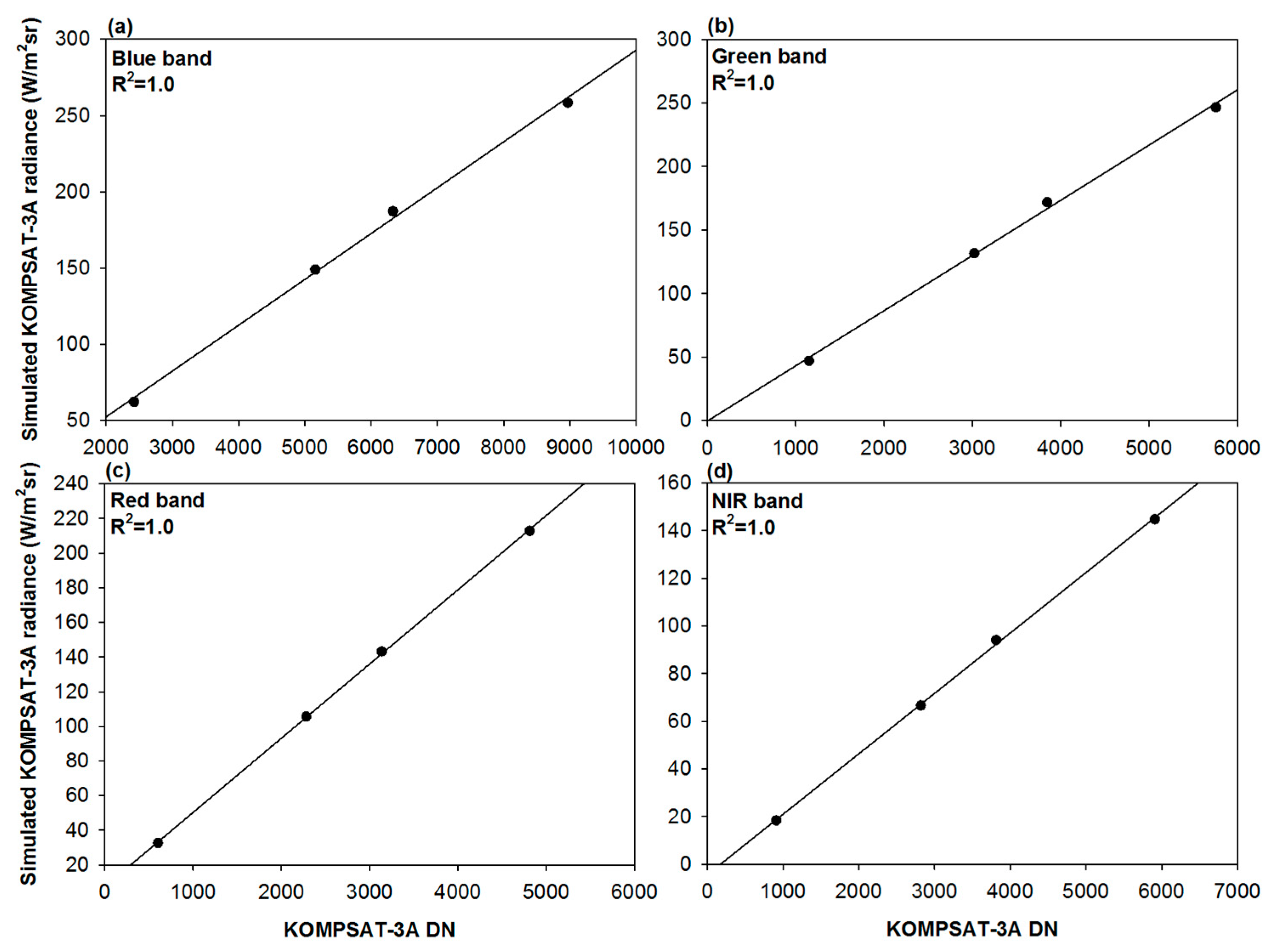
3. Results
4. Discussion
4.1. Approximate Error Budget of Vicarious Calibration for KOMPSAT-3A
4.2. Limitation of Vicarious Calibration of KOMPSAT-3A
5. Summary and Conclusions
Acknowledgments
Author Contributions
Conflicts of Interest
References
- Rees, W.G. Physical Principles of Remote Sensing, 2nd ed.; Cambridge University Press: Cambridge, UK, 2001. [Google Scholar]
- Thuillier, G.; Hersé, M.; Labs, D.; Foujols, T.; Peetermans, W.; Gillotay, D.; Simon, P.C.; Mandel, H. The solar spectral irradiance from 200 to 2400 nm as measured by the SOLSPEC spectrometer from Atlas and Eureca missions. Sol. Phys. 2003, 214, 1–22. [Google Scholar] [CrossRef]
- Liu, C.C.; Kamei, A.; Hsu, K.H.; Tsuchida, S.; Huang, H.M.; Kato, S.; Nakamura, R.; Wu, A.M. Vicarious calibration of the Formasat-2 remote sensing instrument. IEEE Trans. Geosci. Remote Sens. 2010, 48, 2162–2169. [Google Scholar]
- Rao, C.R.N.; Chen, J.; Sullivan, J.T.; Zhang, N. Post-launch calibration of meteorological satellite sensors. Adv. Space Res. 1999, 23, 1357–1365. [Google Scholar] [CrossRef]
- Markham, B.L.; Helder, D.L. Forty-year calibrated record of earth-reflected radiance from Landsat: A review. Remote Sens. Environ. 2012, 122, 30–40. [Google Scholar] [CrossRef]
- Dinguirard, M.; Slater, P.N. Calibration of space-multispectral imaging sensors: A review. Remote Sens. Environ. 1999, 68, 194–205. [Google Scholar] [CrossRef]
- Bowen, H.S. Absolute radiometric calibration of the IKONOS sensor using radiometrically characterized stellar sources. In Proceedings of the Pecora 15/Land Satellite Information IV/ISPRS Commission I/FIEOS 2002 Conference, Denver, CO, USA, 10–15 November 2002.
- Pagnutti, M.; Ryan, R.E.; Kelly, M.; Holekamp, K.; Zanoni, V.; Thome, K.; Schiller, S. Radiometric characterization of IKONOS multispectral imagery. Remote Sens. Environ. 2003, 88, 53–68. [Google Scholar] [CrossRef]
- Teillet, P.M.; Fedosejevs, G.; Thome, K.J.; Barker, J.L. Impacts of spectral band difference effects on radiometric cross-calibration between satellite sensors in the solar-reflective spectral domain. Remote Sens. Environ. 2007, 110, 393–409. [Google Scholar] [CrossRef]
- Mattar, C.; Hernández, J.; Artigas, A.S.; Alarcón, C.D.; Guerra, L.O.; Inzunza, M.; Tapia, D.; Lavín, E.E. A first in-flight absolute calibration of the Chilean Earth Observation satellite. ISPRS J. Photogramm. Remote Sens. 2014, 92, 16–25. [Google Scholar] [CrossRef]
- Kerola, D.X.; Bruegge, C.J.; Gross, H.N.; Helmlinger, M.C. On-orbit calibration of the EO-1 Hyperion and Advanced Land Imager (ALI) sensors using the LED Spectrometer (LSpec) automated facility. IEEE Trans. Geosci. Remote Sens. 2009, 47, 1244–1255. [Google Scholar] [CrossRef]
- Seo, S.B. Relative compensation method for degradation of visible detectors using improved direct histogram specification. Electron. Lett. 2014, 50, 446–447. [Google Scholar] [CrossRef]
- Ham, S.H.; Sohn, B.J. Assessment of the calibration performance of satellite visible channels using cloud targets: Application to Meteosat-8/9 and MTSAT-1R. Atmos. Chem. Phys. 2010, 10, 11131–11149. [Google Scholar] [CrossRef]
- Chavez, P.S. Image-based atmospheric corrections revisited and improved. Photogramm. Eng. Remote Sens. 1996, 62, 1025–1036. [Google Scholar]
- Kim, J.G.; Sohn, B.J.; Chung, E.S.; Chun, H.W. Simulation of TOA visible radiance for the ocean target and its possible use for satellite sensor calibration. Korean J. Remote Sens. 2008, 24, 535–549. [Google Scholar]
- Vermote, E.F.; Tanré, D.; Deuzé, J.L.; Herman, M.; Morcette, J.J. Second simulation of the satellite signal in the solar spectrum, 6S: An overview. IEEE Trans. Geosci. Remote Sens. 1997, 35, 675–686. [Google Scholar] [CrossRef]
- Yeom, J.M.; Hwang, J.; Jin, C.G.; Han, K.S. Radiometric characteristics of KOMPSAT-3 multispectral images using the spectra of well-known surface tarps. IEEE Trans. Geosci. Remote Sens. 2016, 54, 5914–5924. [Google Scholar] [CrossRef]
- Nandy, P.; Thome, K.; Biggar, S. Characterization and field use of a CCD camera system for retrieval of bidirectional reflectance distribution function. J. Geophys. Res. 2001, 106, 11957–11966. [Google Scholar] [CrossRef]
- Pagnutti, M.; Holekamp, K.; Blonski, S.; Sellers, R.; Davis, B.; Zanoni, V. Measurement sets and sites commonly used for characterizations. ISPRS Arch. 2002, XXXIV, 6. [Google Scholar]
- Feng, M.; Sexton, J.O.; Huang, C.; Masek, J.G.; Vermote, E.F.; Gao, F.; Narasimhan, R.; Channan, S.; Wolfe, R.E.; Townshend, J.R. Global surface reflectance products from Landsat: Assessment using coincident MODIS observations. Remote Sens. Environ. 2013, 134, 276–293. [Google Scholar] [CrossRef]
- Kotchenova, S.Y.; Vermote, E.F.; Matarrese, R.; Klemm, F.J. Validation of a vector version of the 6S radiative transfer code for atmospheric correction of satellite data. Part I: Path radiance. Appl. Opt. 2006, 45, 6762–6774. [Google Scholar] [CrossRef] [PubMed]
- Seidel, F.C.; Kokhanovsky, A.A.; Schaepman, M.E. Fast and simple model for atmospheric radiative transfer. Atmos. Meas. Tech. 2010, 3, 1129–1141. [Google Scholar] [CrossRef]
- Vermote, E.F.; Kotchenova, S. Atmospheric correction for the monitoring of land surfaces. J. Geophys. Res. 2008, 113, D23S90. [Google Scholar] [CrossRef]
- Second Simulation of a Satellite Signal in the Solar Spectrum-Vector (6SV). Available online: http://6s.ltdri.org/files/tutorial/6S_Manual_Part_1.pdf (accessed on 3 February 2017).
- Clark, B.; Suomalainen, J.; Pellikka, P. The selection of appropriate spectrally bright pseudo-invariant ground targets for use in empirical line calibration of SPOT satellite imagery. ISPRS J. Photogramm. Remote. Sens. 2011, 66, 429–445. [Google Scholar] [CrossRef]
- Wu, A.; Li, Z.; Cihlar, J. Effects of land cover type and greenness on advanced very high resolution radiometer bidirectional reflectances: Analysis and removal. J. Geophys. Res. 1995, 100, 9179–9192. [Google Scholar] [CrossRef]
- Georgiev, G.T.; Butler, J.J. Laboratory-based bidirectional reflectance distribution functions of radiometric tarps. Appl. Opt. 2008, 47, 3313–3323. [Google Scholar] [CrossRef] [PubMed]
- Feingersh, T.; Dorigo, W.; Richter, R.; Dor, E.B. A new model-driven correction factor for BRDF effects in HRS data. In Proceedings of the EARSel Workshop, Warsaw, Poland, 27–30 April 2005.
- Hwang, J.S. Absolute measurement of hyperspectral and angular reflection. Appl. Opt. 2014, 53, 6216–6221. [Google Scholar] [CrossRef] [PubMed]
- Feingersh, T.; Schläpfer, D.; Bor, E.B. Towards operational BRDF correction for imaging spectrometry data. In Proceedings of the 6th EARSeL SIG IS Workshop, Tel Aviv, Israel, 16–18 March 2009.
- Harrison, L.; Michalsky, J.; Berndt, J. Automated multifilter rotating shadow-band radiometer: An instrument for optical depth and radiation measurements. Appl. Opt. 1994, 33, 5118–5125. [Google Scholar] [CrossRef] [PubMed]
- Alexandrov, M.D.; Schmid, B.; Turner, D.D.; Cairns, B.; Oinas, V.; Lacis, A.A.; Gutman, S.I.; Westwater, E.R.; Smirnov, A.; Eilers, J. Columnar water vapor retrievals from multifilter rotating shadowband radiometer data. J. Geophys. Res. 2009, 114, D02306. [Google Scholar] [CrossRef]
- Koontz, A.; Flynn, C.; Hodges, G.; Michalsky, J.; Barnard, J. Aerosol Optical Depth Value-Added Product; United States Department of Energy: Washington, DC, USA, 2013.
- Lee, K.H.; Li, Z.; Cribb, M.C.; Liu, J.; Wang, L.; Zheng, Y.; Xia, X.; Chen, H.; Li, B. Aerosol optical depth measurements in eastern China and a new calibration method. J. Geophys. Res. 2009, 115. [Google Scholar] [CrossRef]
- Forgan, B.W. Sun Photometer Calibration by the Ratio Langley Method, in Baseline Atmospheric Program; Forgan, B.W., Fraser, P.J., Eds.; Bureau of Meteorology: Melbourne, Australia, 1988; pp. 22–26.
- Hansen, J.E.; Travis, L.D. Light scattering in planetary atmospheres. Space Sci. Rev. 1974, 16, 527–610. [Google Scholar] [CrossRef]
- Alexandrov, M.D.; Lacis, A.A.; Carlson, B.E.; Cairns, B. Remote sensing of atmospheric aerosols and trace gases by means of multifilter rotating shadowband radiometer. Part I: Retrieval algorithms. J. Atmos. Sci. 2002, 59, 524–543. [Google Scholar] [CrossRef]
- Nicolet, M. The solar spectral irradiance and its action in the atmospheric photo dissociation processes. Planet. Space Sci. 1981, 29, 951–974. [Google Scholar] [CrossRef]
- Vandaele, A.C.; Hermans, C.; Fally, S.; Carleer, M.; Colin, R.; Merienne, M.F.; Jenouvrier, A.; Coquart, B. High-resolution Fourier transform measurement of the NO2 visible and near-infrared absorption cross sections: Temperature and pressure effects. J. Geophys. Res. 2002, 107, 43–48. [Google Scholar] [CrossRef]
- Gaskill, J.D. Linear Systems Fourier Transforms and Optics; John Wiley: New York, NY, USA, 1978. [Google Scholar]
- Du, H.; Voss, K.J. Effects of point-spread function on calibration and radiometric accuracy of CCD camera. Appl. Opt. 2004, 43, 665–670. [Google Scholar] [CrossRef] [PubMed]
- Huang, C.; Townshend, J.R.G.; Liang, S.; Kalluri, S.N.V.; DeFries, R.S. Impact of sensor’s point spread function on land cover characterization: Assessment and deconvolution. Remote Sens. Environ. 2002, 80, 203–212. [Google Scholar] [CrossRef]
- Murchie, S.; Robinson, M.; Hawkins, S.E., III; Harch, A.; Helfenstein, P.; Thomas, P.; Peacock, K.; Owen, W.; Heyler, G.; Murphy, P.; et al. Inflight calibration of the NEAR multispectral imager. Icarus 1999, 140, 66–91. [Google Scholar] [CrossRef]
- Li, H.; Robinson, M.S.; Murchie, S. Preliminary remediation of scattered light in NEAR MSI images. Icarus 2002, 155, 244–252. [Google Scholar] [CrossRef]
- Gunn, J.E.; Stryker, L.L. Stellar spectrophotometric atlas, 3130 < 1 < 10800 A. Astrophys. J. Suppl. Ser. 1983, 52, 121–153. [Google Scholar]
- Alexandrov, M.D.; Lacis, A.A.; Carlson, B.E.; Cairns, B. Characterization of atmospheric aerosols using MFRSR measurements. J. Geophys. Res. 2008, 113, D08204. [Google Scholar] [CrossRef]
- TOMS Ozone Algorithm Theoretical Basis Document. Available online: http://projects.knmi.nl/omi/documents/data/OMI_ATBD_Volume_2_V2.pdf (accessed on 3 February 2017).
- Pahlevan, N.; Lee, Z.; Wei, J.; Schaaf, C.B.; Schott, J.R.; Berk, A. On-orbit radiometric characterization of OLI (Landsat-8) for applications in aquatic remote sensing. Remote Sens. Environ. 2014, 154, 272–284. [Google Scholar] [CrossRef]
- Thome, K.J.; Bigger, S.F.; Wisniewski, W. Cross comparison of EO-1 sensors and other earth resources sensors to Landsat-7 ETM+ using Railroad Valley Playa. IEEE Trans. Geosci. Remote Sens. 2003, 41, 1180–1188. [Google Scholar] [CrossRef]
- Chander, G.; Xiong, X.; Angal, A.; Choi, J. Monitoring on-orbit calibration stability of the Terra MODIS and Landsat 7 ETM+ sensors using pseudo-invariant test sites. Remote Sens. Environ. 2010, 114, 935–939. [Google Scholar] [CrossRef]
- Chander, G.; Mishra, N.; Helder, D.L.; Aaron, D.B.; Amit, A.; Choi, T.; Doelling, D.R. Applications of Spectral Band Adjustment Factors (SBAF) for cross-calibration. IEEE Trans. Geosci. Remote Sens. 2013, 51, 1267–1281. [Google Scholar] [CrossRef]
- Lachérade, S.; Fougnie, B.; Henry, P.; Gamet, P. Cross calibration over desert sites: Description, methodology, and operational implementation. IEEE Trans. Geosci. Remote Sens. 2013, 51, 1098–1113. [Google Scholar] [CrossRef]
- Mishra, N.; Helder, D.L.; Angal, A.; Choi, T.; Xiong, X. Absolute calibration of optical satellite sensors using Libya 4 pseudo invariant calibration site. Remote Sens. 2014, 6, 1327–1346. [Google Scholar] [CrossRef]
- Mishra, N.; Haque, M.O.; Leigh, L.; Aaron, D.; Helder, D.; Markham, B. Radiometric cross calibration of Landsat 8 Operational Land Imager(OLI) and Landsat 7 Enhanced Thematic Mapper Plus (ETM+). Remote Sens. 2014, 6, 12619–12638. [Google Scholar] [CrossRef]
- Henry, P.; Dinguirard, M.; Bidilis, M. SPOT multitemporal calibration over stable desert areas. In Proceedings of the SPIE International Symposium of Aerospace Remote Sensing, Orlando, FL, USA, 12–16 April 1993.
- Cabot, F.; Hagolle, O.; Cosnefroy, H.; Briottet, X. Intercalibration using desertic sites as a reference target. In Proceedings of the Geoscience and Remote Sensing Symposium, Seattle, WA, USA, 6–10 July 1998.
- Cosnefroy, H.; Leroy, M.; Briottet, X. Selection and characterization of Saharan and Arabian desert sites for the calibration of optical satellite sensors. Remote Sens. Environ. 1996, 58, 101–114. [Google Scholar] [CrossRef]
- Henry, P.; Chander, G.; Fougnie, B.; Thomas, C.; Xiong, X. Assessment of spectral band impact in intercalibration over desert sites using simulation based on EO-1 Hyperion data. IEEE Trans. Geosci. Remote Sens. 2013, 51, 1297–1308. [Google Scholar] [CrossRef]


| Mission Characteristic | Information |
|---|---|
| Design lifetime | 4 years |
| Orbit altitude | 528 km |
| Swath width | ≥12 km (at nadir) |
| Ground sample distance | PAN: 0.55 m (altitude 528 km) |
| MS: 2.2 m (altitude 528 km) | |
| Spectral bands | Pan 450–900 nm |
| Blue 450–520 nm | |
| Green 520–600 nm | |
| Red 630–690 nm | |
| NIR 760–900 nm | |
| Radiometric Resolution | 14 bit |
| Modulation Transfer Function (MTF) | PAN ≥ 10% |
| MS ≥ 13% | |
| Signal-to-Noise Ratio (SNR) | 100 |
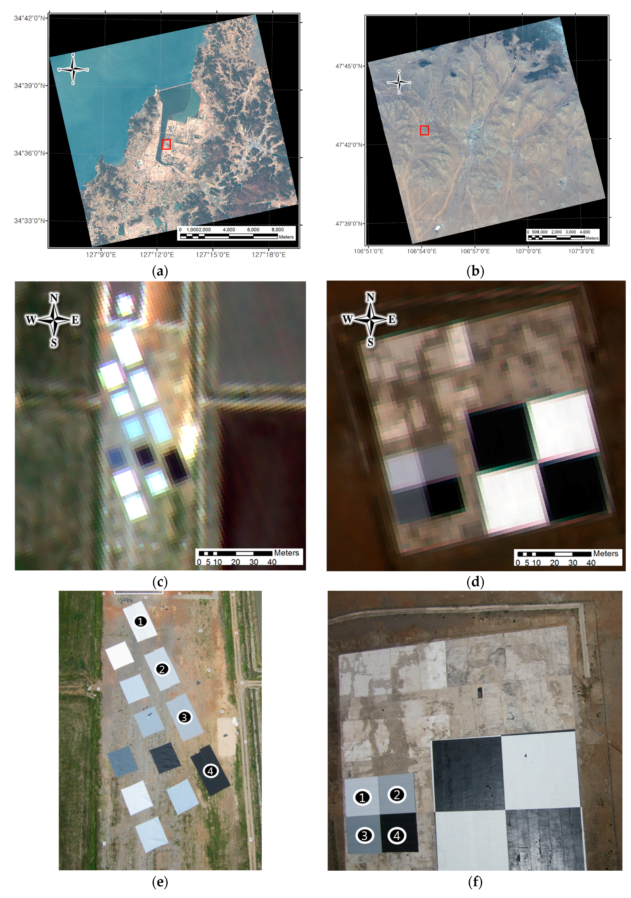
| Site | Date | Overpass Time (UTC) | Solar Zenith | Solar Azimuth | Viewing Zenith | Viewing Azimuth |
|---|---|---|---|---|---|---|
| Goheung, South Korea | 27 May 2015 | 04:43:42 | 21.29 | 236.04 | 9.92 | 261.39 |
| Zuunmod, Mongolia | 18 June 2015 | 05:47:01 | 26.58 | 208.74 | 2.76 | 78.60 |
| Date | Aerosol Optical Depth (550 nm) | Water Vapor (g/cm2) | Ozone (cm-atm) |
|---|---|---|---|
| 27 May 2015 | 0.12 | 0.38 | 287.03 |
| 18 June 2015 | 0.07 | 0.99 | 301.07 |
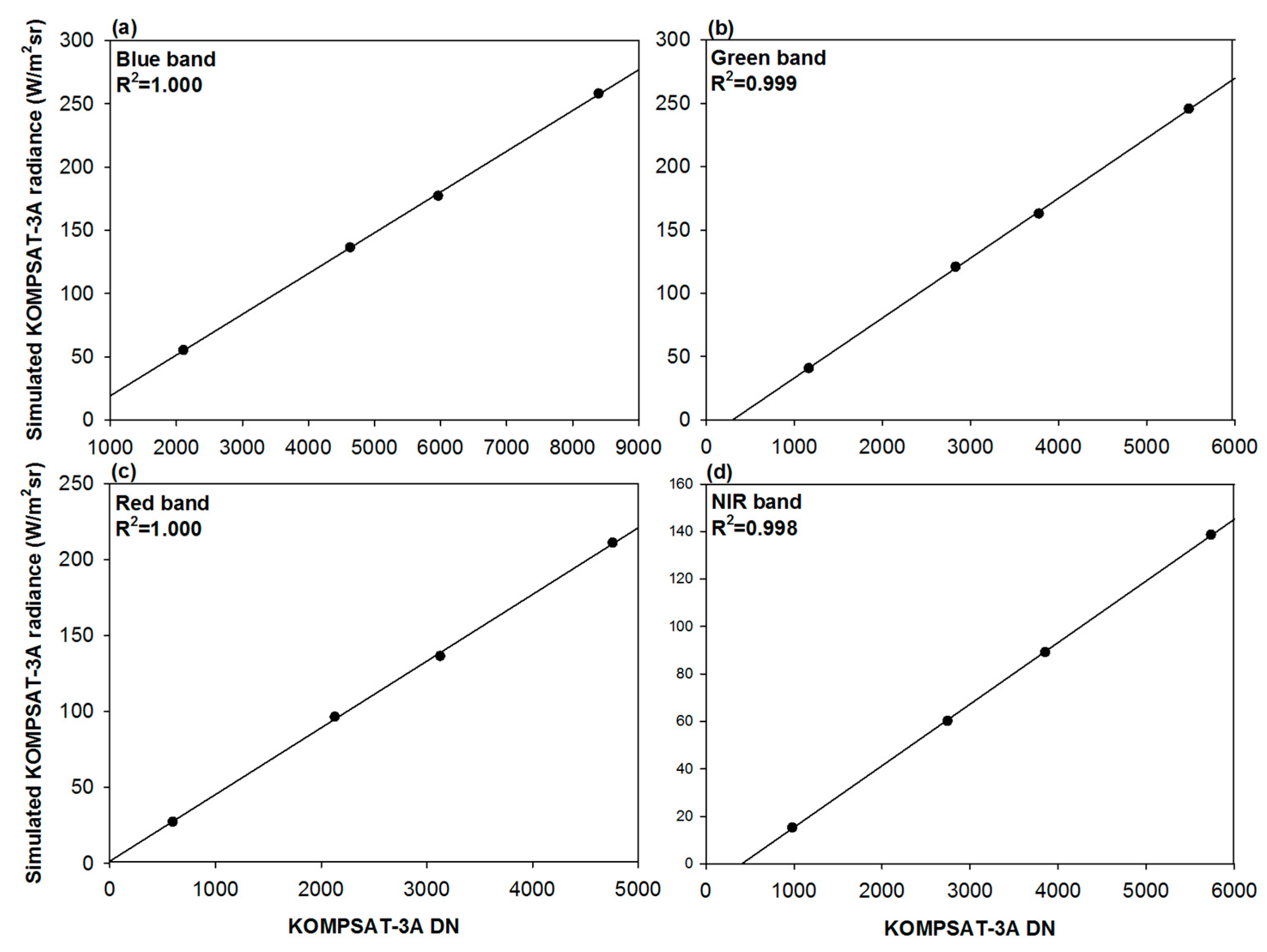
| Spectral Band | Scale Factor (ANIF-Corrected) | R2 (ANIF-Corrected) |
|---|---|---|
| Blue | 0.0285 (0.0289) | 0.999 (1.000) |
| Green | 0.0429 (0.0434) | 1.000 (1.000) |
| Red | 0.0446 (0.0450) | 1.000 (1.000) |
| NIR | 0.0242 (0.0244) | 1.000 (1.000) |
| Spectral Band | Scale Factor | R2 | Gain Ratio between First and Second Field Campaign (ANIF-Corrected) |
|---|---|---|---|
| Blue | 0.0301 | 1.000 | 0.947 (0.960) |
| Green | 0.0438 | 0.999 | 0.979 (0.991) |
| Red | 0.0443 | 1.000 | 1.006 (1.015) |
| NIR | 0.0235 | 0.998 | 1.030 (1.038) |
| Accuracy (%) | Radiance Error (%) | |
|---|---|---|
| Relative radiometric correction | 5 | 5 |
| Solar irradiance data | 3 | 3 |
| Surface reflectance measurement | 1 | 1 |
| Laboratory-based BRDF measurements | 2.5 | 2.5 |
| ASD FieldSpec® 3 instrument | 1 | 1 |
| 6S Radiative transfer | 1 | 1 |
| Aerosol optical depth from MFRSR | 1 | <1 |
| Total ozone from OMI ozone | 2 | <1 |
| Column water vapor amounts from MFRSR | 10 | <1 |
| Combined error | ~6.8 |
© 2017 by the authors. Licensee MDPI, Basel, Switzerland. This article is an open access article distributed under the terms and conditions of the Creative Commons Attribution (CC BY) license ( http://creativecommons.org/licenses/by/4.0/).
Share and Cite
Yeom, J.-M.; Hwang, J.; Jung, J.-H.; Lee, K.-H.; Lee, C.-S. Initial Radiometric Characteristics of KOMPSAT-3A Multispectral Imagery Using the 6S Radiative Transfer Model, Well-Known Radiometric Tarps, and MFRSR Measurements. Remote Sens. 2017, 9, 130. https://doi.org/10.3390/rs9020130
Yeom J-M, Hwang J, Jung J-H, Lee K-H, Lee C-S. Initial Radiometric Characteristics of KOMPSAT-3A Multispectral Imagery Using the 6S Radiative Transfer Model, Well-Known Radiometric Tarps, and MFRSR Measurements. Remote Sensing. 2017; 9(2):130. https://doi.org/10.3390/rs9020130
Chicago/Turabian StyleYeom, Jong-Min, Jisoo Hwang, Jae-Heon Jung, Kwon-Ho Lee, and Chang-Suk Lee. 2017. "Initial Radiometric Characteristics of KOMPSAT-3A Multispectral Imagery Using the 6S Radiative Transfer Model, Well-Known Radiometric Tarps, and MFRSR Measurements" Remote Sensing 9, no. 2: 130. https://doi.org/10.3390/rs9020130
APA StyleYeom, J.-M., Hwang, J., Jung, J.-H., Lee, K.-H., & Lee, C.-S. (2017). Initial Radiometric Characteristics of KOMPSAT-3A Multispectral Imagery Using the 6S Radiative Transfer Model, Well-Known Radiometric Tarps, and MFRSR Measurements. Remote Sensing, 9(2), 130. https://doi.org/10.3390/rs9020130