Bidirectional-Convolutional LSTM Based Spectral-Spatial Feature Learning for Hyperspectral Image Classification

Abstract

This paper proposes a novel deep learning framework named bidirectional-convolutional long short term memory (Bi-CLSTM) network to automatically learn the spectral-spatial features from hyperspectral images (HSIs). In the network, the issue of spectral feature extraction is considered as a sequence learning problem, and a recurrent connection operator across the spectral domain is used to address it. Meanwhile, inspired from the widely used convolutional neural network (CNN), a convolution operator across the spatial domain is incorporated into the network to extract the spatial feature. In addition, to sufficiently capture the spectral information, a bidirectional recurrent connection is proposed. In the classification phase, the learned features are concatenated into a vector and fed to a Softmax classifier via a fully-connected operator. To validate the effectiveness of the proposed Bi-CLSTM framework, we compare it with six state-of-the-art methods, including the popular 3D-CNN model, on three widely used HSIs (i.e., Indian Pines, Pavia University, and Kennedy Space Center). The obtained results show that Bi-CLSTM can improve the classification performance by almost $1.5\%$ as compared to 3D-CNN.

1. Introduction

Current hyperspectral sensors can acquire images with high spectral and spatial resolutions simultaneously. For example, the Airborne Visible/Infrared Imaging Spectrometer (AVIRIS) sensor covers 224 continuous spectral bands across the electromagnetic spectrum with a spatial resolution of 3.7 m. Such rich information has been successfully used in various applications such as national defense, urban planning, precision agriculture and environment monitoring [1].

For these applications, an essential step is image classification, whose purpose is to identify the label of each pixel. Hyperspectral image (HSI) classification is a challenging task. Two important issues exist [2,3]. The first one is the curse of dimensionality. HSI provides very high-dimensional data with hundreds of spectral channels ranging from the visible to the short wave-infrared region of the electromagnetic spectrum. These high-dimensional data with limited numbers of training samples can easily result in the Hughes phenomenon [4], which means that the classification accuracy starts to decrease when the number of features exceeds a threshold. The other one is the use of spatial information. The improvement of spatial resolutions may increase spectral variations among intra-class pixels while decreasing spectral variations among inter-class pixels [5,6]. Thus, only using spectral information is not enough to obtain a satisfying result.

To solve the first issue, a widely used method is to project the original data into a low-dimensional subspace, in which most of the useful information can be preserved. In the existing literature, large amounts of works have been proposed [7,8,9,10]. They can be roughly divided into two categories: unsupervised feature extraction (FE) methods and supervised ones. The unsupervised methods attempt to reveal low-dimensional data structures without using any label information of training samples. These methods retain overall structure of data and do not focus on separating information of samples. Typical methods include but are not limited to principal component analysis (PCA) [7], neighborhood preserving embedding (NPE) [11], and independent component analysis (ICA) [12]. Different from these, the aim of supervised learning methods is to explore the information of labeled data to learn a discriminant subspace. One typical method is linear discriminant analysis (LDA) [13,14], which aims to maximize the inter-class distance and minimize the intra-class distance. In [8], a non-parametric weighted FE (NWFE) method was proposed. NWFE extends LDA by integrating nonparametric scatter matrices with training samples around the decision boundary [8]. Local Fisher discriminant analysis (LFDA) was proposed in [15], which extends the LDA by assigning greater weights to closer connecting samples.

To address the second issue, many works have been proposed to incorporate the spatial information into the spectral information [16,17,18]. This is because the coverage area of one kind of material or one object usually contains more than one pixel. Current spatial-spectral feature fusion methods can be categorized into three classes: feature-level fusion, decision-level fusion, and regularization-level fusion [3]. For feature-level fusion, one often extracts the spatial features and the spectral features independently and then concatenates them into a vector [5,19,20,21]. However, the direct concatenation will lead to a high-dimensional feature space. For decision-level fusion, multiple results are first derived using the spatial and spectral information, respectively, and then combined according to some strategies such as the majority voting strategy [22,23,24]. For regularization-level fusion, a regularizer representing the spatial information is incorporated into the original object function. For example, in [25,26], Markov random field (MRF) modeling, the joint prior probabilities of each pixel and its spatial neighbors were incorporated into the Bayesian classifier as a regularizer. Although this method works well in capturing the spatial information, optimizing the objective function in MRF is time-consuming, especially on high-resolution data.

Recently, deep learning (DL) has attracted much attention in the field of remote sensing [27,28,29,30]. The core idea of DL is to automatically learn high-level semantic features from data itself in a hierarchical manner. In [31,32], the autoencoder model has been successfully used for HSI classification. In general, the inputs of the autoencoder model are a high-dimensional vector. Thus, to learn the spatial features from HSIs, an alternative method is flattening a local image patch into a vector and then feeding it into the model. However, this method may destroy the two-dimensional (2D) structure of images, leading to the loss of spatial information. Similar issues can be found in the deep belief network (DBN) [33]. To address this issue, convolutional neural network (CNN) based deep models have been popularly used [2,34]. They directly take the original image or the local image patch as network inputs, and use local-connected and weight sharing structure to extract the spatial features from HSIs. In [2], the authors designed a CNN network with three convolutional layers and one fully-connected layer. In addition, the input of the network is the first principal component of HSIs extracted by PCA. Although the experimental results demonstrate that this model can successfully learn the spatial feature of HSIs, it may fail to extract the spectral features. Recently, a three-dimensional (3D) CNN model was proposed in [34]. In order to extract the spectral-spatial features from HSIs, the authors consider the 3D image patches as the input of the network. This complex structure will inevitably increase the amount of parameters, easily leading to the overfitting problem with a limited number of training samples.

In this paper, we propose a bidirectional-convolutional long short term memory (Bi-CLSTM) network to address the spectral-spatial feature learning problem. Specifically, we regard all the spectral bands as an image sequence, and model their relationships using a powerful LSTM network [35]. Similar to other fully-connected networks such as autoencoder and DBN, LSTM can not capture the spatial information of HSIs. Inspired from [36], we replace the fully-connected operators in the network by convolutional operators, resulting in a convolutional LSTM (CLSTM) network. Thus, CLSTM can simultaneously learn the spectral and spatial features. In addition, LSTM assumes that previous states affect future states, while the spectral channels in the sequence are correlated with each other. To address this issue, we further propose a Bi-CLSTM network. During the training process of the Bi-CLSTM network, we adopt two tricks to alleviate the overfitting problem. They are dropout and data augmentation operations.

To sum up, the main contributions of this paper are as follows. First, we consider images in all the spectral bands as an image sequence, and use LSTM to effectively model their relationships; second, considering the specific characteristics of hyperspectral images, we further propose a unified framework to combine the merits of LSTM and CNN for spectral-spatial feature extraction.

2. Review of RNN and LSTM

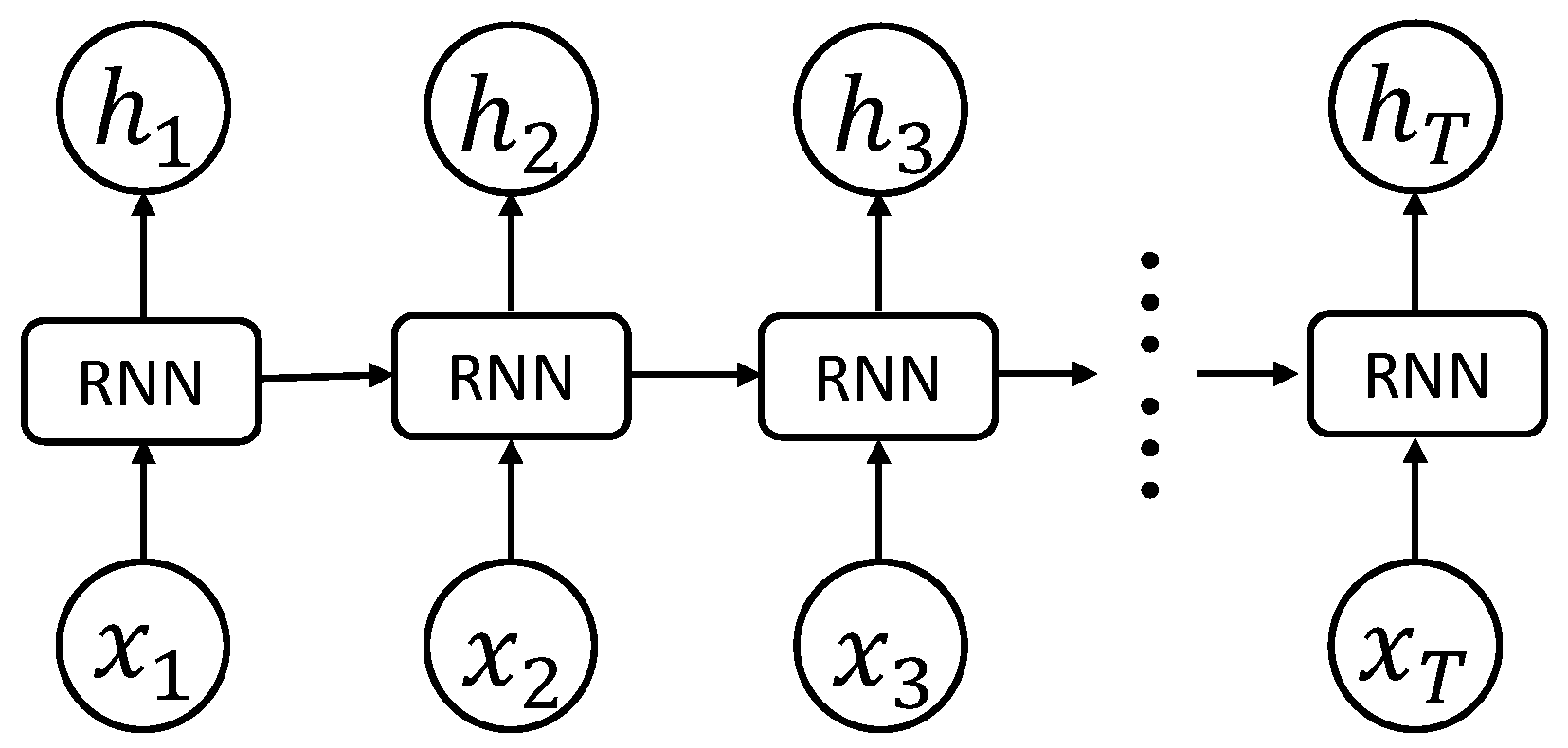
Recurrent neural network (RNN) [37,38] is an extension of traditional neural networks and used to address the sequence learning problem. Unlike the feedforward neural network, RNN adds recurrent edges to connect the neuron to itself across time so that it can model a probability distribution over sequence data. Figure 1 demonstrates an example of RNN. The input of the network is a sequence data $\{x_1,x_2,\dots ,x_T\}$. The node updates its hidden state $h_t$, given its previous state $h_{t-1}$ and present input $x_t$, by

$$h_t=\sigma (W_{hx}{x}_t+W_{hh}{h}_{t-1}+b),$$

(1)

where $W_{hx}$ is the weight between the input node and the recurrent hidden node, $W_{hh}$ is the weight between the recurrent hidden node and itself from the previous time step, and b and $\sigma$ are bias and nonlinear activation function, respectively.

Figure 1. The structure of RNN.

As an important branch of the deep learning family, RNNs have recently shown promising results in many machine learning and computer vision tasks [39,40]. However, it has been observed that training RNN models to model the long-term sequence data is difficult. As can be seen from Equation (1), the contribution of recurrent hidden node $h_m$ at time m to itself $h_n$ at time n may approach infinity or zero as the time interval increases whether $|W_{hh}|<1$ or $|W_{hh}|>1$. This will lead to the gradient vanishing and exploding problem [41]. To address this issue, Hochreiter and Schmidhuber proposed LSTM to replace the recurrent hidden node by a memory cell. The memory cell contains a node with a self-connected recurrent edge of a fixed weight one, ensuring that the gradient can pass across many time steps without vanishing or exploding. The LSTM unit consists of four important parts: input gate $i_t$, output gate $o_t$, forget gate $f_t$, and candidate cell value ${\tilde{C}}_t$. Based on these parts, memory cell and output can be computed by:

$$\begin{array}{c}{f}_t=\sigma (W_{hf}·h_{t-1}+W_{xf}·x_t+b_f)\hfill \\ i_t=\sigma (W_{hi}·h_{t-1}+W_{xi}·x_t+b_i)\hfill \\ {\tilde{C}}_t=\tanh (W_{hC}·h_{t-1}+W_{xC}·x_t+b_C)\hfill \\ C_t=f_t\circ C_{t-1}+i_t\circ {\tilde{C}}_t\hfill \\ o_t=\sigma (W_{ho}·h_{t-1}+W_{xo}·x_t+b_o)\hfill \\ h_t=o_t\circ \tanh \left(C_t\right),\hfill \end{array}$$

(2)

where $\sigma$ is the logistic sigmoid function, ‘·’ is a matrix multiplication operator, ‘∘’ is a dot product operator, and $b_f$, $b_i$, $b_C$ as well as $b_o$ are bias terms. The weight matrix subscripts have obvious meanings. For instance, $W_{hi}$ is the hidden-input gate matrix, and $W_{xo}$ is the input-output gate matrix etc.

3. Methodology

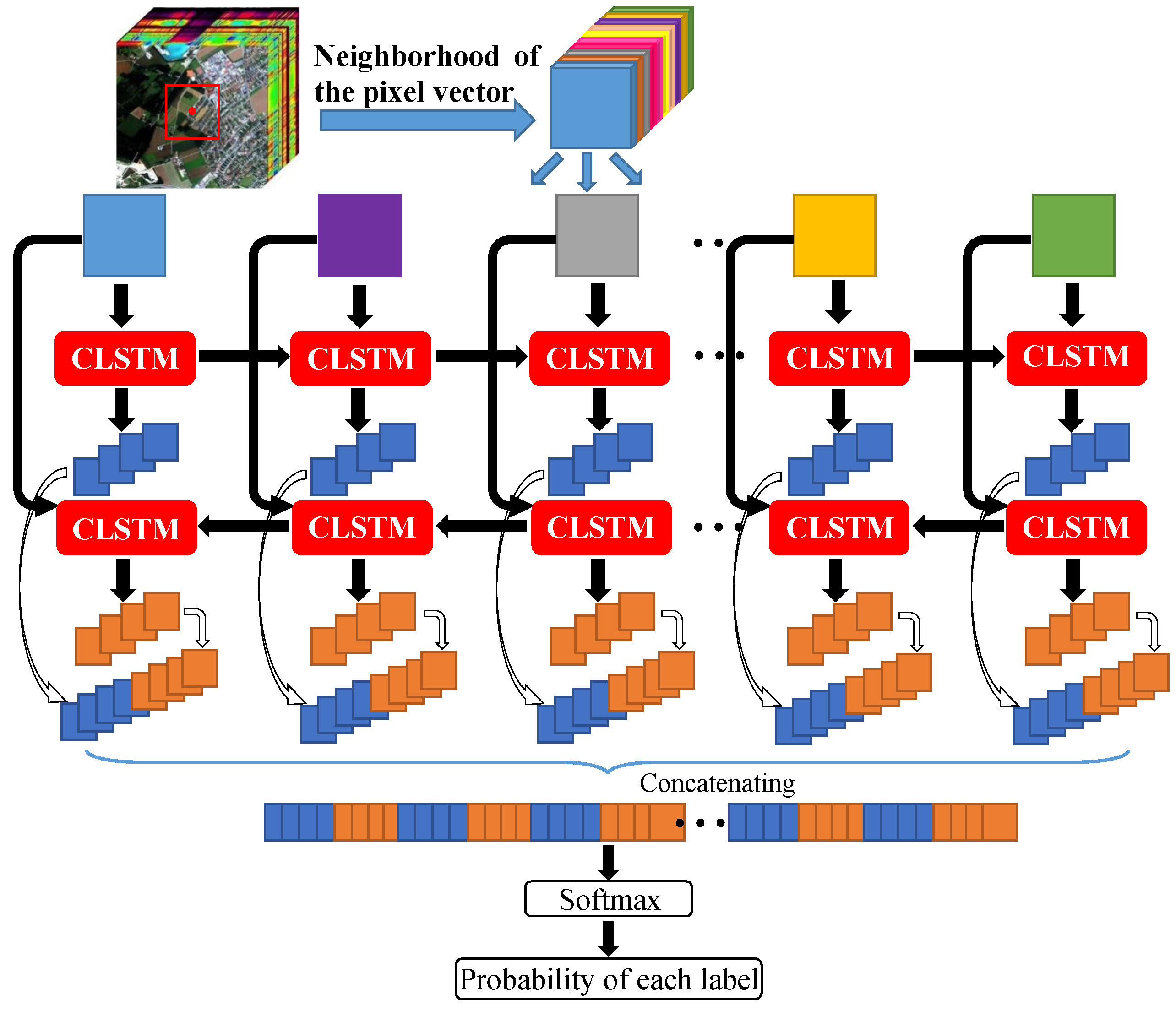
The flowchart of the proposed Bi-CLSTM model is shown in Figure 2. Suppose an HSI can be represented as a 3D matrix $\mathbf{X}\in {\mathbf{R}}^{m\times n\times l}$ with $m\times n$ pixels and l spectral channels. Given a pixel at the spatial position $\left(i,j\right)$ where $1\le i\le m$ and $1\le j\le n$, we can choose a small sub-cube ${\mathbf{X}}_{ij}\in {\mathbf{R}}^{p\times p\times l}$ centered at it. The goal of Bi-CLSTM is to learn the most discriminative spectral-spatial information from ${\mathbf{X}}_{ij}$. Such information is the final feature representation for the pixel at the spatial position $\left(i,j\right)$. If we split the sub-cube across the spectral channels, then ${\mathbf{X}}_{ij}$ can be considered as an l-length sequence $\{(x_{ij}^1,x_{ij}^2,\cdots ,x_{ij}^l)|x_{ij}^k\in {\mathbf{R}}^{p\times p\times 1},1\le k\le l\}$. The image patches in the sequence are fed into the CLSTM one by one to extract the spectral feature via a recurrent operator and the spatial feature via a convolution operator simultaneously.

Figure 2. Flowchart of the Bi-CLSTM network for HSI classification. For a given pixel, a local cube surrounding it is first extracted, and then unfolded across the spectral domain. The unfolded images are fed into the Bi-CLSTM network one by one.

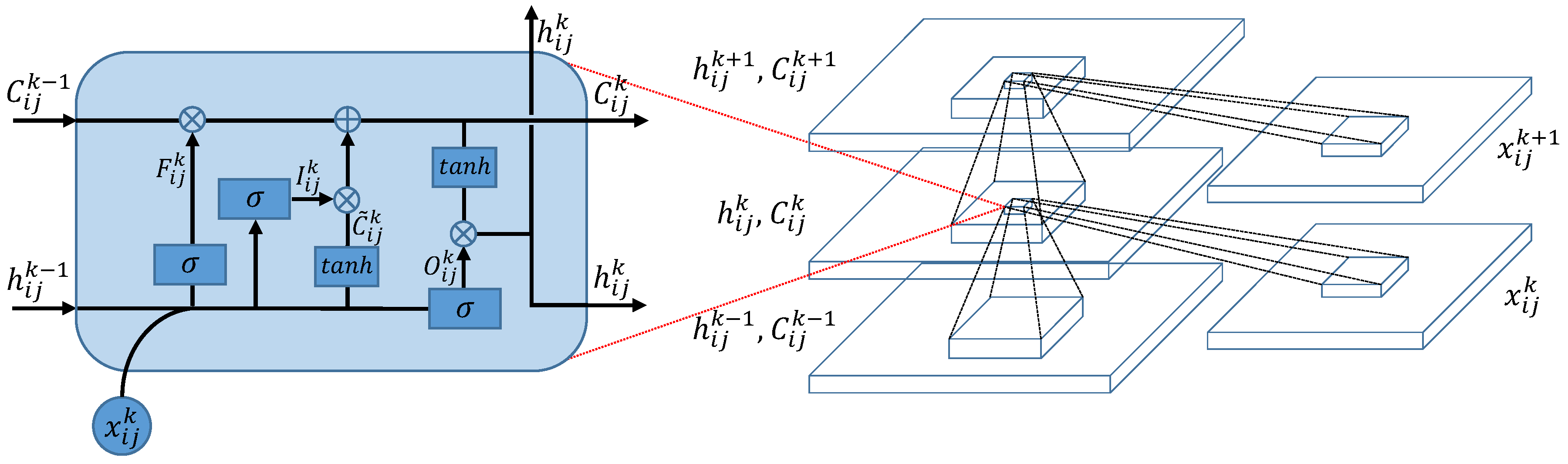
CLSTM is a modification of LSTM, which replaces the fully-connected operators by convolutional operators [36]. The structure of CLSTM is shown in Figure 3, where the left side zooms in its core computation unit, called a memory cell. In the memory cell, ‘⊗’ and ‘⊕’ represent dot product and matrix addition, respectively. For the k-th image patch $x_{ij}^k$ in the sequence ${\mathbf{X}}_{ij}$, CLSTM firstly decides what information to throw away from the previous cell state $C_{ij}^{k-1}$ via the forget gate $F_{ij}^k$. The forget gate pays attention to $h_{ij}^{k-1}$ and $x_{ij}^k$, and outputs a value between 0 and 1 after an activation function. Here, 1 represents “keep the whole information” and 0 represents “throw away the information completely”. Secondly, CLSTM needs to decide what new information to store in the current cell state $C_{ij}^k$. This includes two parts: first, the input gate $I_{ij}^k$ decides what information to update by the same way as forget gate; second, the memory cell creates a candidate value ${\tilde{C}}_{ij}^k$ computed by $h_{ij}^{k-1}$ and $x_{ij}^k$. After finishing these two parts, CLSTM multiplies the previous memory cell state $C_{ij}^{k-1}$ by $F_{ij}^k$, adds the product to $I_{ij}^k\circ {\tilde{C}}_{ij}^k$, and updates the information $C_{ij}^k$. Finally, CLSTM decides what information to output via the cell state $C_{ij}^k$ and output gate $O_{ij}^k$. The above process can be formulated as the following equations:

$$\begin{array}{c}{F}_{ij}^k=\sigma (W_{hf}\ast h_{ij}^{k-1}+W_{xf}\ast x_{ij}^k+b_f)\hfill \\ I_{ij}^k=\sigma (W_{hi}\ast h_{ij}^{k-1}+W_{xi}\ast x_{ij}^k+b_i)\hfill \\ {\tilde{C}}_{ij}^k=\tanh (W_{hc}\ast h_{ij}^{k-1}+W_{xc}\ast x_{ij}^k+b_c)\hfill \\ C_{ij}^k=F_{ij}^k\circ C_{ij}^{k-1}+I_{ij}^k\circ {\tilde{C}}_{ij}^k\hfill \\ O_{ij}^k=\sigma (W_{ho}\ast h_{ij}^{k-1}+W_{xo}\ast x_{ij}^k+b_o)\hfill \\ h_{ij}^k=O_{ij}^k\circ \tanh (C_{ij}^k),\hfill \end{array}$$

(3)

where $\sigma$ is the logistic sigmoid function, ‘∗’ is a convolutional operator, ‘∘’ is a dot product, and $b_f,b_i,b_c$ and $b_o$ are bias terms. The weight matrix subscripts have the obvious meaning. For example, $W_{hi}$ is the hidden-input gate matrix, and $W_{xo}$ is the input-output gate matrix etc. To implement the convolutional and recurrent operator in CLSTM simultaneously, the spatial size of $h_{ij}^{k-1}$ and $C_{ij}^{k-1}$ must be the same as that of $x_{ij}^k$ (we use zero-padding [42] to ensure that input will keep the original spatial size after convolution operation).

Figure 3. The structure of CLSTM.

In the existing literature [43,44,45], LSTM has been well acknowledged as a powerful network to address the orderly sequence learning problem based on the assumption that previous states will affect future states. However, different from the traditional sequence learning problem, the spectral channels in the sequence are correlated with each other. In [46], bidirectional recurrent neural networks (Bi-RNN) was proposed to use both latter and previous information to model sequential data. Motivated by it, we use a Bi-CLSTM network shown in Figure 2 to sufficiently extract the spectral feature. Specifically, the image patches are fed into the CLSTM network one by one with a forward and a backward sequence, respectively. After that, we can acquire two spectral-spatial feature sequences. In the classification stage, they are concatenated into a vector denoted as G and a Softmax layer is used to obtain the probability of each class that the pixel belongs to. Softmax function ensures the activation of each output unit sums to 1, so that we can deem the output as a set of conditional probabilities. Given the vector G, the probability that the input belongs to category c equals

$$\begin{array}{c}\hfill {\mathbf{P}}_{ij}(y=c|G,W,b)=\frac{e^{W_{c}G+b_c}}{{\sum }_m{e}^{W_{m}G+b_m}},\end{array}$$

(4)

where W and b are weights and biases of the Softmax layer and the summation is over all the output units. The pseudocode for the Bi-CLSTM model is given in Algorithm 1, where we use simplified variables to make the procedure clear.

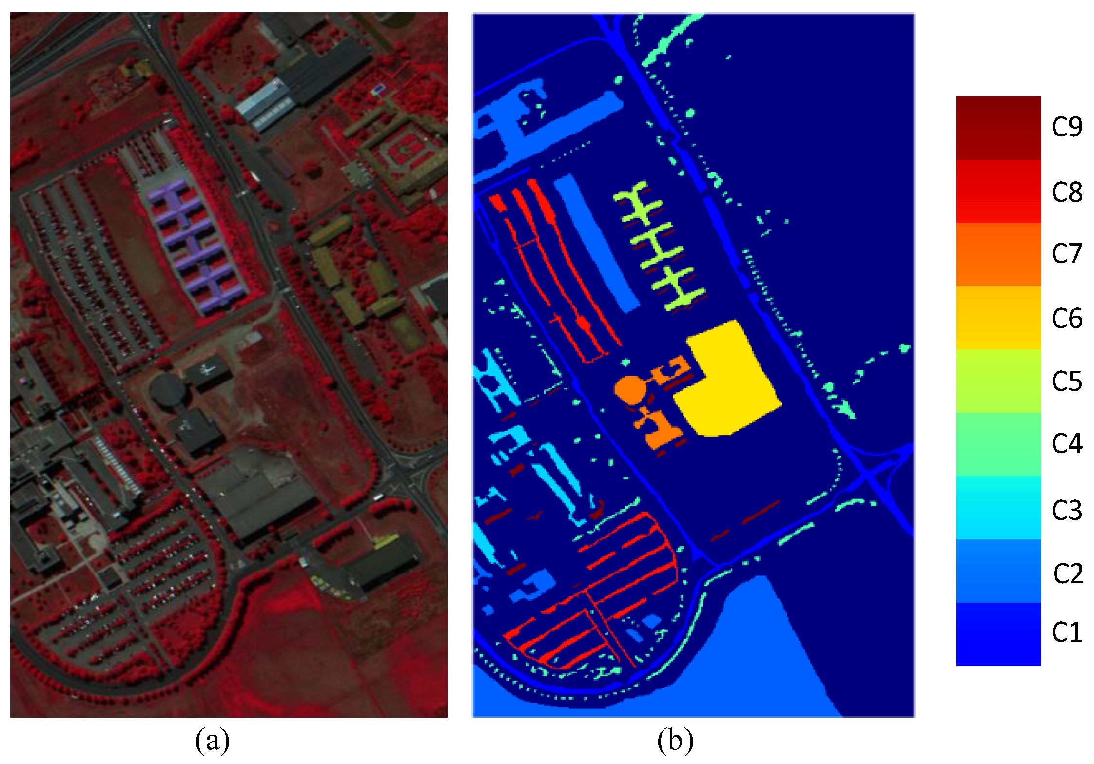
It is well known that the performance of DL algorithms depends on the number of training samples. However, there often exists a small number of available samples in HSIs. To this end, we adopt two data augmentation methods. They are flipping and rotating operators. Specifically, we rotate the HSI patches by 90, 180, and 270 degrees anticlockwise and flip them horizontally and vertically. Furthermore, we rotate the horizontally and vertically flipped patches by 90 degrees separately. 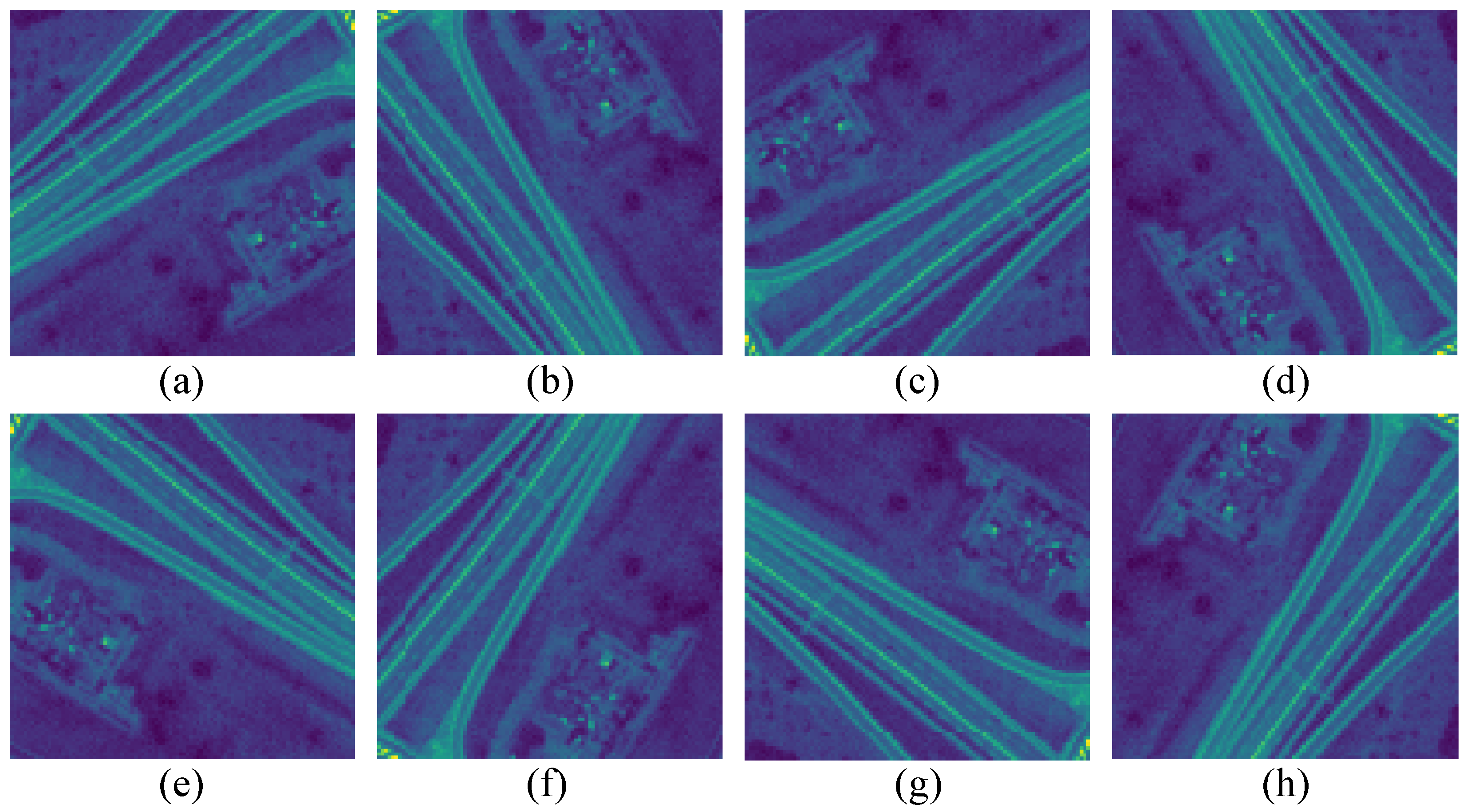Figure 4 shows some examples of flipping and rotating operators. As a result, the number of training samples can be increased by eight times. In addition, the data augmentation method, dropout [47] is also used to improve the performance of Bi-CLSTM. We set some outputs of neurons to zeros, which means that these neurons do not propagate any information forward or participate in the back-propagation learning algorithm. Every time an input is sampled, network drops neurons randomly to form different structures. In the next section, we will validate the effectiveness of data augmentation and dropout methods.

Figure 4. The example of data augmentation. (a) the original image; (b–d) the images after rotation of 90, 180, and 270 degrees anticlockwise; (e) vertical flip of (c); (f) horizontal flip of (d); (g–h) the horizontally and vertically flipped images of (c,d).

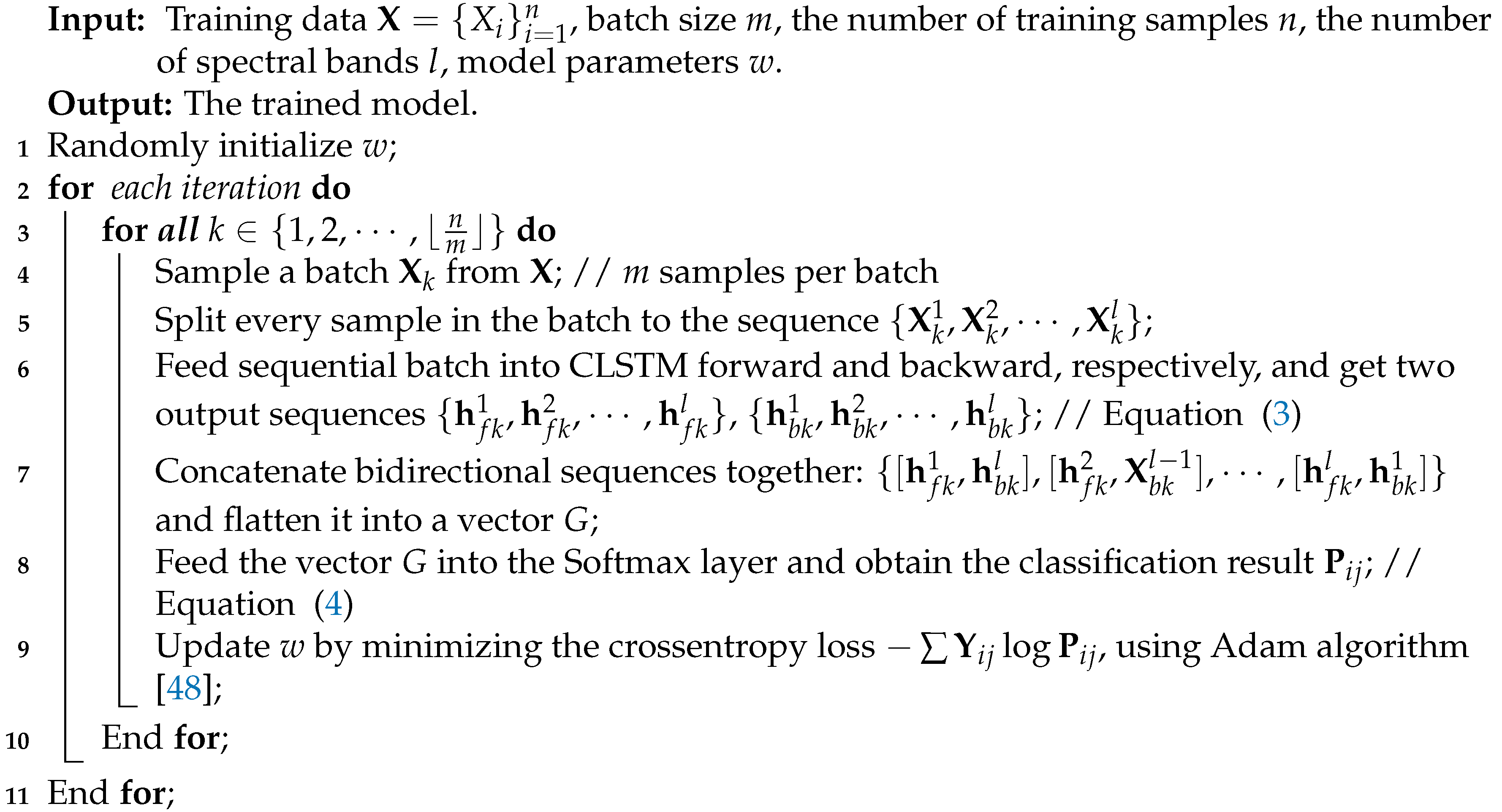
Algorithm 1: Algorithm for the Bi-CLSTM model.

4. Experimental Results

4.1. Datasets

We test the proposed Bi-CLSTM model on three HSIs, which are widely used to evaluate classification algorithms.

• Indian Pines: The first dataset was acquired by the AVIRIS sensor over the Indian Pine test site in northwestern Indiana, USA, on 12 June 1992 and it contains 224 spectral bands. We utilize 200 bands after removing four bands containing zero values and 20 noisy bands affected by water absorption. The spatial size of the image is $145\times 145$ pixels, and the spatial resolution is 20 m. The false-colour composite image and the ground truth map are shown in Figure 5. The available number of samples is 10,249 ranging from 20 to 2455 in each class.
  

  Figure 5. Indian Pines scene dataset. (a) false-color composite of the Indian Pines scene; (b) ground truth map containing 16 mutually exclusive land cover classes.
• Pavia University: The second dataset was acquired by the reflective optics system imaging spectrometer (ROSIS) sensor during a flight campaign over Pavia, northern Italy, on 8 July 2002. The original image was recorded with 115 spectral channels ranging from 0.43 $\mathsf{\mu }$m to 0.86 $\mathsf{\mu }$m. After removing noisy bands, 103 bands are used. The image size is $610\times 340$ pixels with a spatial resolution of 1.3 m. A three band false-colour composite image and the ground truth map are shown in Figure 6. In the ground truth map, there are nine different classes of land covers with more than 1000 labeled pixels for each class.
  

  Figure 6. Pavia University scene dataset. (a) false-color composite of the Pavia University scene; (b) ground truth map containing nine mutually exclusive land cover classes.
• Kennedy Space Center (KSC): The third dataset was acquired by the AVIRIS sensor over Kennedy Space Center (KSC), Florida, on 23 March 1996. It contains 224 spectral bands. We utilize 176 bands of them after removing bands with water absorption and low signal noise ratio. The spatial size of the image is $512\times 614$ pixels, and the spatial resolution is 18 m. Discriminating different land covers in this dataset is difficult due to the similarity of spectral signatures among certain vegetation types. For classification purposes, thirteen classes representing the various land-cover types that occur in this environment are defined. Figure 7 demonstrates a false-colour composite image and the ground truth map.
  

  Figure 7. KSC dataset. (a) false-color composite of the KSC. (b) ground truth map containing 13 mutually exclusive land cover classes.

For Indian Pines and KSC datasets, we randomly select $10\%$ pixels from each class as the training set, and use the remaining pixels as the testing set. The same as the experiments in [3,49], we randomly choose 3921 pixels as the training set and the rest of pixels as the testing set for the Pavia University dataset. The detailed numbers of training and testing samples are listed from Table 1, Table 2 and Table 3.

Table 1. Number of pixels for training/testing and the total number of pixels for each class in the Indian Pines ground truth map.

No.	Class	Total	Training	Test
C1	Alfalfa	46	5	41
C2	Corn-notill	1428	143	1285
C3	Corn-mintill	830	83	747
C4	Corn	237	24	213
C5	Grass-pasture	483	48	435
C6	Grass-trees	730	73	657
C7	Grass-pasture-mowed	28	3	25
C8	Hay-windrowed	478	48	430
C9	Oats	20	2	18
C10	Soybean-notill	972	97	875
C11	Soybean-mintill	2455	246	2209
C12	Soybean-clean	593	59	534
C13	Wheat	205	21	184
C14	Woods	1265	127	1138
C15	Buildings-Grass-Trees-Drives	386	39	347
C16	Stone-Steel-Towers	93	9	84

Table 2. Number of pixels for training/testing and the total number of pixels for each class in the Pavia University ground truth map.

No.	Class	Total	Training	Test
C1	Asphalt	6631	548	6083
C2	Meadows	18,649	540	18,109
C3	Gravel	2099	392	1707
C4	Trees	3064	524	2540
C5	Painted metal sheets	1345	265	1080
C6	Bare Soil	5029	532	4497
C7	Bitumen	1330	375	955
C8	Self-Blocking Bricks	3682	514	3168
C9	Shadows	947	231	716

Table 3. Number of pixels for training/testing and the total number of pixels for each class in the KSC ground truth map.

No.	Class	Total	Training	Test
C1	Scrub	761	76	685
C2	Willow swamp	243	24	219
C3	Cabbage palm hammock	256	26	230
C4	Cabbage palm/oak hammock	252	25	227
C5	Slash pine	161	16	145
C6	Oak/broadleaf hammock	229	23	206
C7	Hardwood swamp	105	11	94
C8	Graminoid marsh	431	43	388
C9	Spartina marsh	520	52	468
C10	Cattail marsh	404	40	364
C11	Salt marsh	419	42	377
C12	Mud flats	503	50	453
C13	Water	927	93	834

4.2. Experimental Setup

We compared the proposed Bi-CLSTM model with several FE methods, including regularized local discriminant embedding (RLDE) [50], matrix-based discriminant analysis (MDA) [3], 2D-CNN, 3D-CNN, LSTM [49], and CNN+LSTM. We train DL models on a single TITAN X GPU and implement them in TensorFlow. Additionally, we also directly use the original pixels as a benchmark. The optimal reduced dimension for RLDE is chosen from $[2,30]$. For MDA, the optimal window size is selected from a given set $\{3,5,7,9,11\}$. For 2D-CNN and 3D-CNN, we take the same configuration as described in [34]. For LSTM, we build a single recurrent layer with 128 hidden nodes. For CNN+LSTM, we apply CNN to extract spatial features from each band and then employ LSTM to fuse them. The configuration of CNN is the same as that in [34], and the number of hidden nodes in LSTM is 128. For Bi-CLSTM, we build a bidirectional network with two CLSTM layers to extract features. Similar to CNN, the convolution operation are followed by max-pooling in Bi-CLSTM, and we empirically set the size of convolution kernel to $3\times 3$ and the number of convolution kernel to 32. Without loss of generality, we initialize the state of CLSTM to zeros. The detailed configuration of Bi-CLSTM is listed in Table 4. The dimension of each layer in Bi-CLSTM is detailed in Table 5, where l and C indicate the number of spectral bands and classes, respectively, and F-CLSTM and B-CLSTM indicate forward and backward CLSTM, respectively. When training Bi-CLSTM, we set the loss function to cross entropy and optimize it by Adam algorithm with a learning rate of ${10}^{-3}$.

Table 4. Detailed configuration of Bi-CLSTM.

Direction	Convolution	MaxPooling	Dropout
Forward	3 × 3 × 32	2 × 2	0.6
Backward	3 × 3 × 32	2 × 2	0.6

Table 5. The dimension of each layer in Bi-CLSTM.

Layer	Input	Conv-Output	Pool-Output
F-CLSTM	$64\times 64\times l$	$32\times 32\times l$	$16\times 16\times l$
B-CLSTM	$64\times 64\times l$	$32\times 32\times l$	$16\times 16\times l$
Layer	Input	Output
Softmax	$2\times 16\times 16\times l$	C

In order to reduce the effects of random selection, all the algorithms are repeated five times and the average results are reported. The classification performance is evaluated by the overall accuracy (OA), the average accuracy (AA), the per-class accuracy, and the Kappa coefficient $\kappa$. OA defines the ratio between the number of correctly classified pixels to the total number of pixels in the testing set, AA refers to the average of accuracies in all classes, and $\kappa$ is the percentage of agreement corrected by the number of agreements that would be expected purely by chance. Clearly, larger values of the three metrics correspond to better performance.

4.3. Parameter Selection

There are four important influence factors in Bi-CLSTM, including dropout, data augmentation, network framework, and the size of input image patches. Firstly, to find the optimal size of image patches, we fix the other three factors and select the size from four candidate values $\{8,16,32,64\}$. Table 6 demonstrates the effects of different sizes on OA of the KSC dataset. From this table, we can observe that OA increases as the patch size increases, and $64\times 64$ size can achieve a high enough accuracy. Since larger size will dramatically increase the computation time and the accuracy improvement is limited, the optimal size can be chosen as $64\times 64$.

Table 6. OA of Bi-CLSTM with different sizes of input image patches on the KSC dataset.

Size	$8\times 8$	$16\times 16$	$32\times 32$	$64\times 64$
OA(%)	96.12	97.78	98.57	99.13

Secondly, to investigate the performance of bidirectional network structure, we fix the other influence factors and compare forward CLSTM (F-CLSTM) with Bi-CLSTM on the KSC dataset. Here, F-CLSTM is a forward network with the same configuration as Bi-CLSTM listed in Table 4. As shown in Table 7, the bidirectional network indeed outperforms the ordinary forward network. This result certifies the effectiveness of Bi-CLSTM as compared to the forward CLSTM. Finally, we also validate the effectiveness of dropout and data augmentation operators. We set the probability of dropout to the common value 0.6, and fix the other influence factors. Table 8 reports the OA values with or without dropout operator on the KSC dataset. It can be observed that using dropout can significantly improve the accuracy from 94.41% to 99.13%. Similarly, we expand the number of training samples by eight times as described in Section II and fix the other influence factors. Table 8 demonstrates that data augmentation can improve the accuracy from 95.07% to 99.13%.

Table 7. OA of F-CLSTM and Bi-CLSTM on the KSC dataset.

Network	F-CLSTM	Bi-CLSTM
OA(%)	95.44	99.13

Table 8. OA of Bi-CLSTM on the KSC dataset with and without dropout and data augmentation.

Operator	Yes	No
Dropout	99.13	94.41
Data augmentation	99.13	95.07

4.4. Performance Comparison

To demonstrate the superiority of the proposed Bi-CLSTM model, we quantitatively and qualitatively compare it with the aforementioned methods. Table 9 reports the quantitative results acquired by eight methods on the Indian Pines dataset. From these results, we can observe that most of the DL methods perform better than traditional methods. For 2D-CNN, it only uses the principal component of all spectral bands, leading to the loss of spectral information. Therefore, the performance obtained by 2D-CNN is inferior to that by MDA. For LSTM, it takes the hyperspectral pixel vector as input without considering spatial-domain information, achieving the worst performance among all methods. Different from 2D-CNN and LSTM, CNN+LSTM attempts to feed spatial features from each band into the LSTM model to capture the spectral information, obtaining better performance than MDA. This is because, as a neural network, CNN+LSTM is able to capture the nonlinear distribution property of hyperspectral data, while the linear FE method MDA may fail. Nevertheless, the spectral FE and spatial FE processes are independent, making the trained parameters in CNN+LSTM may be not the optimal ones. 3D-CNN and Bi-CLSTM can address this issue by extracting spectral and spatial features simultaneously, and achieve the higher OA, AA, and $\kappa$ than CNN+LSTM. For 3D-CNN, a specific number of spectral bands is taken as an input of the network every time. Therefore, it cannot learn the relationships between non-adjacent spectral bands. Via recurrent connections, Bi-CLSTM can model the correlations across all the spectral bands. Thus, compared to 3D-CNN, Bi-CLSTM improves OA from 95.30% to 96.78%. Figure 8 demonstrates the classification maps achieved by eight different methods on the Indian Pines dataset. It can be observed that Bi-CLSTM obtains more homogeneous maps than other methods.

Table 9. OA, AA, per-class accuracy (%), $\kappa$ and standard deviations after five runs performed by eight methods on the Indian Pines dataset using $10\%$ pixels from each class as the training set.

Label	Original	RLDE	MDA	2D-CNN	3D-CNN	LSTM	CNN+LSTM	Bi-CLSTM
OA	77.44 ± 0.71	80.97 ± 0.60	92.31 ± 0.43	90.14 ± 0.78	95.30 ± 0.34	72.22 ± 3.65	94.15 ± 0.84	96.78 ± 0.35
AA	74.94 ± 0.99	80.94 ± 2.12	89.54 ± 3.08	85.66 ± 3.24	92.02 ± 2.09	61.72 ± 3.38	90.30 ± 4.13	94.47 ± 0.83
$\kappa$	74.32 ± 0.78	78.25 ± 0.70	91.21 ± 0.50	88.73 ± 0.90	94.65 ± 0.39	68.24 ± 4.13	93.50 ± 1.00	96.33 ± 0.40
C1	56.96 ± 10.91	64.78 ± 15.25	73.17 ± 17.92	71.22 ± 15.75	92.68 ± 10.63	25.85 ± 17.47	91.06 ± 7.45	93.66 ± 6.12
C2	79.75 ± 2.77	78.39 ± 1.34	93.48 ± 1.42	90.10 ± 2.33	95.41 ± 2.58	66.60 ± 5.16	94.26 ± 2.58	96.84 ± 2.05
C3	66.60 ± 3.03	68.10 ± 2.16	84.02 ± 3.11	91.03 ± 2.73	96.16 ± 1.82	54.83 ± 8.31	95.29 ± 3.02	97.22 ± 2.02
C4	59.24 ± 7.14	70.80 ± 6.04	83.57 ± 2.23	85.73 ± 5.02	92.49 ± 4.48	43.94 ± 13.29	93.80 ± 7.08	96.71 ± 3.59
C5	90.31 ± 1.45	92.17 ± 1.97	96.69 ± 1.39	83.36 ± 5.75	87.89 ± 3.32	83.45 ± 4.45	84.78 ± 5.45	92.28 ± 3.82
C6	95.78 ± 1.64	94.90 ± 2.04	99.15 ± 0.51	91.99 ± 3.25	95.23 ± 2.21	87.76 ± 4.02	90.87 ± 6.10	99.39 ± 0.61
C7	80.00 ± 7.82	85.71 ± 6.68	93.60 ± 6.07	85.60 ± 12.20	86.67 ± 12.22	23.20 ± 20.47	84.00 ± 11.31	92.00 ± 9.80
C8	97.41 ± 0.84	99.12 ± 0.95	99.91 ± 0.13	97.35 ± 3.75	99.84 ± 0.27	95.40 ± 1.86	99.07 ± 1.57	99.91 ± 0.21
C9	35.00 ± 10.61	73.00 ± 21.10	63.33 ± 24.72	54.45 ± 23.70	72.22 ± 20.03	30.00 ± 15.01	55.56 ± 23.57	76.67 ± 21.66
C10	66.32 ± 3.18	69.73 ± 1.07	82.15 ± 2.23	75.38 ± 8.97	91.24 ± 1.77	71.29 ± 3.97	93.35 ± 5.45	95.93 ± 2.00
C11	70.77 ± 2.42	79.38 ± 0.56	92.76 ± 1.45	94.36 ± 0.48	97.59 ± 0.96	75.08 ± 5.53	98.82 ± 0.35	96.31 ± 1.46
C12	64.42 ± 3.92	72.28 ± 3.42	91.35 ± 2.26	78.73 ± 8.00	93.01 ± 3.09	54.49 ± 8.73	89.78 ± 4.43	93.33 ± 3.12
C13	95.41 ± 2.62	97.56 ± 1.38	99.13 ± 0.49	95.98 ± 4.82	96.56 ± 3.62	91.85 ± 3.90	95.65 ± 3.03	95.76 ± 3.72
C14	92.66 ± 1.77	92.36 ± 0.92	98.22 ± 0.39	96.80 ± 1.08	98.83 ± 0.89	90.37 ± 4.93	95.36 ± 4.35	99.49 ± 0.35
C15	60.88 ± 6.27	67.10 ± 6.39	87.84 ± 4.00	96.54 ± 2.54	90.01 ± 7.21	30.49 ± 2.02	95.53 ± 7.08	98.67 ± 1.11
C16	87.53 ± 1.95	89.68 ± 3.28	94.29 ± 6.43	81.90 ± 17.71	86.51 ± 5.36	62.86 ± 10.43	87.62 ± 4.00	87.38 ± 9.09

Figure 8. Classification maps using eight different methods on the Indian Pines dataset: (a) original; (b) RLDE; (c) MDA; (d) 2D-CNN; (e) 3D-CNN; (f) LSTM; (g) CNN+LSTM; (h) Bi-CLSTM.

Similar results are demonstrated in Table 10 and Figure 9 on the Pavia University Scene dataset. Again, 3D-CNN, CNN+LSTM, and Bi-CLSTM achieve better performance than other methods. Specifically, OA, AA and $\kappa$ obtained by 3D-CNN and CNN+LSTM are higher than MDA, and Bi-CLSTM obtains better performance than 3D-CNN and CNN+LSTM. It is worth noting that the improvement of OA, AA and $\kappa$ from MDA to Bi-CLSTM is not remarkable as those on the Indian Pines dataset because MDA has already obtained a high performance and a further improvement is very difficult. Table 11 and Figure 10 show the classification results of different methods on the KSC dataset. Similar to the other two datasets, Bi-CLSTM achieves the highest OA, AA and $\kappa$ than other methods.

Table 10. OA, AA, per-class accuracy (%), $\kappa$ and standard deviations after five runs performed by eight methods on the Pavia University Scene dataset using 3921 pixels as the training set.

Label	Original	RLDE	MDA	2D-CNN	3D-CNN	LSTM	CNN+LSTM	Bi-CLSTM
OA	89.12 ± 0.26	88.82 ± 0.25	96.95 ± 0.29	96.55 ± 0.85	97.65 ± 0.40	93.20 ± 0.71	97.11 ± 0.95	99.10 ± 0.16
AA	90.50 ± 0.06	90.45 ± 0.06	96.86 ± 0.23	97.19 ± 0.51	97.74 ± 0.48	93.13 ± 0.42	98.27 ± 0.77	99.20 ± 0.17
$\kappa$	85.81 ± 0.32	85.43 ± 0.31	95.93 ± 0.52	95.30 ± 1.13	96.80 ± 0.54	90.43 ± 0.91	96.09 ± 1.29	98.77 ± 0.21
C1	87.25 ± 0.57	87.20 ± 0.52	96.69 ± 0.41	96.72 ± 1.48	95.33 ± 3.73	91.33 ± 2.05	98.54 ± 0.94	98.56 ± 0.58
C2	89.10 ± 0.54	88.40 ± 0.52	97.76 ± 0.47	96.31 ± 1.75	97.99 ± 0.94	94.58 ± 1.77	95.51 ± 1.92	99.23 ± 0.39
C3	81.99 ± 1.05	81.69 ± 0.80	90.69 ± 1.44	97.15 ± 1.58	95.27 ± 1.81	83.93 ± 3.72	97.64 ± 3.68	99.27 ± 0.47
C4	95.65 ± 0.59	95.79 ± 0.56	98.44 ± 0.27	96.16 ± 1.29	98.49 ± 1.07	97.78 ± 2.36	98.80 ± 0.60	98.21 ± 0.92
C5	99.76 ± 0.14	99.87 ± 0.08	100.00 ± 0.00	99.81 ± 0.32	98.67 ± 1.26	99.46 ± 0.24	99.28 ± 0.59	99.87 ± 0.15
C6	88.78 ± 1.01	88.67 ± 0.67	96.26 ± 0.45	94.87 ± 3.62	99.21 ± 0.74	91.73 ± 4.17	98.40 ± 1.05	99.56 ± 0.29
C7	85.92 ± 0.93	86.06 ± 1.04	97.95 ± 0.62	97.44 ± 1.68	97.90 ± 1.36	90.76 ± 2.85	98.91 ± 1.86	99.75 ± 0.30
C8	86.14 ± 1.02	86.42 ± 0.73	93.98 ± 0.97	98.23 ± 0.91	97.84 ± 2.55	88.78 ± 2.44	98.48 ± 1.16	99.82 ± 0.55
C9	99.92 ± 0.05	99.94 ± 0.06	100.00 ± 0.00	98.04 ± 0.96	98.97 ± 0.93	99.83 ± 0.23	98.83 ± 0.90	99.53 ± 0.47

Figure 9. Classification maps using eight different methods on the Pavia University dataset: (a) original; (b) RLDE; (c) MDA; (d) 2D-CNN; (e) 3D-CNN; (f) LSTM; (g) CNN+LSTM; (h) Bi-CLSTM.

Table 11. OA, AA, per-class accuracy (%), $\kappa$ and standard deviations after five runs performed by eight methods on the KSC dataset using $10\%$ pixels from each class as the training set.

Label	Original	RLDE	MDA	2D-CNN	3D-CNN	LSTM	CNN+LSTM	Bi-CLSTM
OA	93.16 ± 0.38	93.50 ± 0.31	96.81 ± 0.17	92.55 ± 0.84	97.14 ± 0.49	84.96 ± 1.26	96.12 ± 0.45	98.29 ± 0.98
AA	89.15 ± 0.55	90.09 ± 0.71	95.30 ± 0.83	89.20 ± 1.50	95.92 ± 0.64	82.87 ± 1.67	94.91 ± 0.86	97.77 ± 1.37
$\kappa$	92.38 ± 0.42	92.77 ± 0.34	96.45 ± 0.18	91.69 ± 0.95	96.82 ± 0.55	83.24 ± 1.41	95.68 ± 0.50	98.10 ± 1.09
C1	95.43 ± 2.54	95.30 ± 1.64	96.93 ± 1.03	94.86 ± 1.30	96.06 ± 1.24	96.53 ± 1.35	96.00 ± 2.53	98.87 ± 1.36
C2	91.44 ± 4.43	92.26 ± 5.48	97.26 ± 1.29	77.53 ± 5.05	98.48 ± 0.95	80.25 ± 2.67	89.04 ± 8.90	93.61 ± 5.93
C3	90.86 ± 6.55	88.44 ± 2.00	98.92 ± 0.30	84.52 ± 5.31	95.79 ± 3.93	95.36 ± 2.89	92.96 ± 6.29	99.35 ± 0.56
C4	79.52 ± 5.74	76.90 ± 5.48	90.31 ± 0.62	77.71 ± 11.85	90.89 ± 5.73	58.00 ± 11.42	87.31 ± 6.13	94.71 ± 2.07
C5	68.20 ± 7.71	77.64 ± 2.45	80.00 ± 7.80	80.97 ± 9.54	80.92 ± 2.87	60.00 ± 11.78	90.48 ± 3.91	97.24 ± 2.93
C6	67.34 ± 3.90	77.82 ± 0.72	92.47 ± 2.40	72.62 ± 14.78	97.25 ± 1.22	60.52 ± 7.35	93.30 ± 2.58	94.54 ± 9.01
C7	84.19 ± 5.33	82.67 ± 16.06	94.68 ± 6.01	93.19 ± 5.35	96.45 ± 6.14	57.45 ± 20.11	99.36 ± 1.43	99.74 ± 0.53
C8	95.17 ± 1.26	91.97 ± 2.39	96.26 ± 4.19	93.87 ± 2.41	96.65 ± 2.11	90.40 ± 4.87	92.11 ± 2.53	97.23 ± 3.16
C9	95.92 ± 1.69	98.08 ± 1.50	99.89 ± 0.15	95.85 ± 3.03	98.22 ± 0.62	92.74 ± 2.10	99.44 ± 1.24	97.81 ± 1.08
C10	96.78 ± 1.56	96.78 ± 1.20	98.35 ± 0.39	96.81 ± 1.79	98.72 ± 0.97	93.96 ± 3.60	95.71 ± 2.53	99.66 ± 0.52
C11	98.14 ± 0.87	98.23 ± 1.38	99.33 ± 0.19	94.27 ± 2.21	99.73 ± 0.46	98.63 ± 1.16	99.84 ± 0.36	98.94 ± 2.12
C12	95.90 ± 1.23	95.39 ± 1.31	94.59 ± 1.72	97.35 ± 2.09	97.86 ± 1.21	93.47 ± 2.63	98.28 ± 2.87	99.28 ± 0.89
C13	100.00 ± 0.00	99.68 ± 0.40	99.94 ± 0.08	100.00 ± 0.00	100.00 ± 0.00	100.00 ± 0.00	100.00 ± 0.00	100.00 ± 0.00

Figure 10. Classification maps using eight different methods on the KSC dataset: (a) original; (b) RLDE; (c) MDA; (d) 2D-CNN; (e) 3D-CNN; (f) LSTM; (g) CNN+LSTM; (h) Bi-CLSTM.

To test the computational efficiency of different deep learning methods, we train and test them on a personal computer with CPU of Intel Core i7-4790 and GPU of GTX TITAN X, using the TensorFlow framework. As shown in Table 12, 3D-CNN and Bi-CLSTM cost more training and testing time than 2D-CNN, LSTM and CNN+LSTM because their inputs are sub-cubes while others are vectors or matrices. In addition, compared to 3D-CNN, training or testing Bi-CLSTM is faster. This is because the convolutional kernel sizes (i.e., $3\times 3\times 32$) in each direction of Bi-CLSTM are smaller than those of 3D-CNN (i.e., $4\times 4\times 32\times 128$), and the depth of Bi-CLSTM is shallower than it.

Table 12. Computation time (min.) of five deep learning methods on three datasets.

Dataset	2D-CNN		3D-CNN		LSTM		CNN+LSTM		Bi-CLSTM
	Train	Test	Train	Test	Train	Test	Train	Test	Train	Test
Indian Pines	10.00	0.07	1435.33	70.57	75.00	0.55	260.00	3.38	535.50	12.62
Pavia University	15.00	0.23	818.33	18.38	85.00	0.52	291.67	4.23	432.00	12.95
KSC	5.00	0.03	183.33	3.73	25.00	0.18	65.00	1.07	112.50	2.65

5. Conclusions

In this paper, we propose a novel bidirectional-convolutional long short term memory (Bi-CLSTM) network to automatically learn the spectral-spatial feature from hyperspectral images (HSIs). The input of the network is the whole spectral channels of HSIs, and a bidirectional recurrent connection operator across them is used to sufficiently explore the spectral information. In addition, motivated by the widely used convolutional neural network (CNN), fully-connected operators in the network are replaced by convolution operators across the spatial domain to capture the spatial information. By conducting experiments on three HSIs collected by different instruments (AVIRIS and ROSIS), we compare the proposed method with several feature extraction methods including deep learning algorithms, i.e., CNN, LSTM and CNN+LSTM. The experimental results indicate that using spatial information improves the classification performance and results in more homogeneous regions in classification maps compared to only using spectral information. In addition, the proposed method can improve the OA, AA, and $\kappa$ on three HSIs as compared to other methods. We also evaluate the influences of different components in the network, including dropout, data augmentation and patch size.

References

- Zhang, S.; Li, S.; Fu, W.; Fang, L. Multiscale Superpixel-Based Sparse Representation for Hyperspectral Image Classification. Remote Sens. 2017, 9, 139. [Google Scholar] [CrossRef]
- Zhao, W.; Du, S. Spectral-Spatial Feature Extraction for Hyperspectral Image Classification: A Dimension Reduction and Deep Learning Approach. IEEE Trans. Geosci. Remote Sens. 2016, 54, 4544–4554. [Google Scholar] [CrossRef]
- Hang, R.; Liu, Q.; Song, H.; Sun, Y. Matrix-Based Discriminant Subspace Ensemble for Hyperspectral Image Spatial-Spectral Feature Fusion. IEEE Trans. Geosci. Remote Sens. 2015, 54, 783–794. [Google Scholar] [CrossRef]
- Hughes, G. On the Mean Accuracy of Statistical Pattern Recognizers. IEEE Trans. Inf. Theory 1968, 14, 55–63. [Google Scholar] [CrossRef]
- Zhang, L.; Zhang, L.; Tao, D.; Huang, X. On Combining Multiple Features for Hyperspectral Remote Sensing Image Classification. IEEE Trans. Geosci. Remote Sens. 2012, 50, 879–893. [Google Scholar] [CrossRef]
- Xu, J.; Hang, R.; Liu, Q. Patch-Based Active Learning PTAL for Spectral-Spatial Classification on Hyperspectral Data. Int. J. Remote Sens. 2014, 35, 1846–1875. [Google Scholar] [CrossRef]
- Palsson, F.; Sveinsson, J.R.; Ulfarsson, M.O.; Benediktsson, J.A. Model-Based Fusion of Multi- and Hyperspectral Images Using PCA and Wavelets. IEEE Trans. Geosci. Remote Sens. 2015, 53, 2652–2663. [Google Scholar] [CrossRef]
- Kuo, B.C.; Landgrebe, D.A. Nonparametric Weighted Feature Extraction for Classification. IEEE Trans. Geosci. Remote Sens. 2004, 42, 1096–1105. [Google Scholar]
- Chen, H.T.; Chang, H.W.; Liu, T.L. Local Discriminant Embedding and Its Variants. In Proceedings of the IEEE Computer Society Conference on Computer Vision and Pattern Recognition, San Diego, CA, USA, 20–25 June 2005; pp. 846–853. [Google Scholar]
- Wang, Q.; Meng, Z.; Li, X. Locality Adaptive Discriminant Analysis for Spectral–Spatial Classification of Hyperspectral Images. IEEE Geosci. Remote Sens. Lett. 2017, 14, 2077–2081. [Google Scholar] [CrossRef]
- He, X.; Cai, D.; Yan, S.; Zhang, H.J. Neighborhood Preserving Embedding. In Proceedings of the Tenth IEEE International Conference on Computer Vision, Beijing, China, 17–21 October 2005; Volume 2, pp. 1208–1213. [Google Scholar]
- Villa, A.; Benediktsson, J.A.; Chanussot, J.; Jutten, C. Hyperspectral Image Classification with Independent Component Discriminant Analysis. IEEE Trans. Geosci. Remote Sens. 2011, 49, 4865–4876. [Google Scholar] [CrossRef]
- Friedman, J.H. Regularized Discriminant Analysis. J. Am. Stat. Assoc. 1989, 84, 165–175. [Google Scholar] [CrossRef]
- Bandos, T.V.; Bruzzone, L.; Camps-Valls, G. Classification of Hyperspectral Images with Regularized Linear Discriminant Analysis. IEEE Trans. Geosci. Remote Sens. 2009, 47, 862–873. [Google Scholar] [CrossRef]
- Sugiyama, M. Dimensionality Reduction of Multimodal Labeled Data by Local Fisher Discriminant Analysis. J. Mach. Learn. Res. 2007, 8, 1027–1061. [Google Scholar]
- Fauvel, M.; Tarabalka, Y.; Benediktsson, J.A.; Chanussot, J. Advances in Spectral-Spatial Classification of Hyperspectral Images. Proc. IEEE 2013, 101, 652–675. [Google Scholar] [CrossRef]
- Sun, L.; Wu, Z.; Liu, J.; Xiao, L. Supervised Spectral-Spatial Hyperspectral Image Classification with Weighted Markov Random Fields. IEEE Trans. Geosci. Remote Sens. 2015, 53, 1490–1503. [Google Scholar] [CrossRef]
- Liu, J.; Wu, Z.; Wei, Z.; Xiao, L.; Sun, L. Spatial-Spectral Kernel Sparse Representation for Hyperspectral Image Classification. IEEE J. Sel. Top. Appl. Earth Obs. Remote Sens. 2013, 6, 2462–2471. [Google Scholar] [CrossRef]
- Fauvel, M.; Benediktsson, J.A.; Chanussot, J.; Sveinsson, J.R. Spectral and Spatial Classification of Hyperspectral Data Using SVMs and Morphological Profiles. IEEE Trans. Geosci. Remote Sens. 2008, 46, 3804–3814. [Google Scholar] [CrossRef]
- Mura, M.D.; Villa, A.; Benediktsson, J.A.; Chanussot, J. Classification of Hyperspectral Images by Using Extended Morphological Attribute Profiles and Independent Component Analysis. IEEE Geosci. Remote Sens. Lett. 2011, 8, 542–546. [Google Scholar] [CrossRef]
- Benediktsson, J.A.; Palmason, J.A.; Sveinsson, J.R. Classification of Hyperspectral Data from Urban Areas Based on Extended Morphological Profiles. IEEE Trans. Geosci. Remote Sens. 2005, 43, 480–491. [Google Scholar] [CrossRef]
- Tarabalka, Y.; Benediktsson, J.A.; Chanussot, J. Spectral-Spatial Classification of Hyperspectral Imagery Based on Partitional Clustering Techniques. IEEE Trans. Geosci. Remote Sens. 2009, 47, 2973–2987. [Google Scholar] [CrossRef]
- Jimenez, L.O.; Rivera-Medina, J.L.; Rodriguez-Diaz, E.; Arzuaga-Cruz, E. Integration of Spatial and Spectral Information by Means of Unsupervised Extraction and Classification for Homogenous Objects Applied to Multispectral and Hyperspectral Data. IEEE Trans. Geosci. Remote Sens. 2005, 43, 844–851. [Google Scholar] [CrossRef]
- Tarabalka, Y.; Benediktsson, J.A.; Chanussot, J.; Tilton, J.C. Multiple Spectral-Spatial Classification Approach for Hyperspectral Data. IEEE Trans. Geosci. Remote Sens. 2010, 48, 4122–4132. [Google Scholar] [CrossRef]
- Jia, X.; Richards, J.A. Managing the Spectral-Spatial Mix in Context Classification Using Markov Random Fields. IEEE Geosci. Remote Sens. Lett. 2008, 5, 311–314. [Google Scholar] [CrossRef]
- Jackson, Q.; Landgrebe, D.A. Adaptive Bayesian Contextual Classification Based on Markov Random Fields. IEEE Trans. Geosci. Remote Sens. 2002, 40, 2454–2463. [Google Scholar] [CrossRef]
- Wu, H.; Prasad, S. Convolutional Recurrent Neural Networks for Hyperspectral Data Classification. Remote Sens. 2017, 9, 298. [Google Scholar] [CrossRef]
- Liang, H.; Li, Q. Hyperspectral Imagery Classification Using Sparse Representations of Convolutional Neural Network Features. Remote Sens. 2016, 8, 99. [Google Scholar] [CrossRef]
- He, Z.; Liu, H.; Wang, Y.; Hu, J. Generative Adversarial Networks-Based Semi-Supervised Learning for Hyperspectral Image Classification. Remote Sens. 2017, 9, 1042. [Google Scholar] [CrossRef]
- Ding, C.; Li, Y.; Xia, Y.; Wei, W.; Zhang, L.; Zhang, Y. Convolutional Neural Networks Based Hyperspectral Image Classification Method with Adaptive Kernels. Remote Sens. 2017, 9, 618. [Google Scholar] [CrossRef]
- Chen, Y.; Lin, Z.; Zhao, X.; Wang, G.; Gu, Y. Deep Learning-Based Classification of Hyperspectral Data. IEEE J. Sel. Top. Appl. Earth Obs. Remote Sens. 2014, 7, 2094–2107. [Google Scholar] [CrossRef]
- Tao, C.; Pan, H.; Li, Y.; Zou, Z. Unsupervised Spectral-Spatial Feature Learning with Stacked Sparse Autoencoder for Hyperspectral Imagery Classification. IEEE Geosci. Remote Sens. Lett. 2015, 12, 2438–2442. [Google Scholar]
- Chen, Y.; Zhao, X.; Jia, X. Spectral-Spatial Classification of Hyperspectral Data Based on Deep Belief Network. IEEE J. Sel. Top. Appl. Earth Obs. Remote Sens. 2015, 8, 2381–2392. [Google Scholar] [CrossRef]
- Chen, Y.; Jiang, H.; Li, C.; Jia, X. Deep Feature Extraction and Classification of Hyperspectral Images Based on Convolutional Neural Networks. IEEE Trans. Geosci. Remote Sens. 2016, 54, 6232–6251. [Google Scholar] [CrossRef]
- Hochreiter, S.; Schmidhuber, J. Long Short-Term Memory. Neural Comput. 1997, 9, 1735. [Google Scholar] [CrossRef] [PubMed]
- Xingjian, S.; Chen, Z.; Wang, H.; Yeung, D.Y.; Wong, W.K.; Woo, W.C. Convolutional LSTM network: A machine learning approach for precipitation nowcasting. In Advances in Neural Information Processing Systems; 2015; pp. 802–810. Available online: papers.nips.cc/paper/5955-convolutional-lstm-network-a-machine-learning-approach-for-precipitation-nowcasting.pdf (accessed on 15 December 2017).
- Williams, R.; Zipser, D. A Learning Algorithm for Continually Running Fully Recurrent Neural Networks. Neural Comput. 1989, 1, 270–280. [Google Scholar] [CrossRef]
- Rodriguez, P.; Wiles, J.; Elman, J.L. A Recurrent Neural Network That Learns to Count. Connect. Sci. 1999, 11, 5–40. [Google Scholar] [CrossRef]
- Cho, K.; Merrienboer, B.V.; Gulcehre, C.; Bahdanau, D.; Bougares, F.; Schwenk, H.; Bengio, Y. Learning Phrase Representations Using RNN Encoder-Decoder for Statistical Machine Translation. arXiv. 2014. Available online: https://arxiv.org/pdf/1406.1078 (accessed on 15 December 2017).
- Ranzato, M.; Szlam, A.; Bruna, J.; Mathieu, M.; Collobert, R.; Chopra, S. Video (Language) Modeling: A Baseline for Generative Models of Natural Videos. arXiv. 2014. Available online: https://arxiv.org/pdf/1412.6604 (accessed on 15 December 2017).
- Hochreiter, S.; Bengio, Y.; Frasconi, P.; Schmidhuber, J. Gradient Flow in Recurrent Nets: The Difficulty of Learning Long-Term Dependencies. In A Field Guide to Dynamical Recurrent Neural Networks; IEEE Press, 2001; Available online: www.bioinf.jku.at/publications/older/ch7.pdf (accessed on 15 December 2017).
- Dumoulin, V.; Visin, F. A Guide to Convolution Arithmetic for Deep Learning. arXiv. 2016. Available online: https://arxiv.org/pdf/1603.07285 (accessed on 15 December 2017).
- Sutskever, I.; Vinyals, O.; Le, Q.V. Sequence to Sequence Learning with Neural Networks. In Advances in Neural Information Processing Systems; 2014; pp. 3104–3112. Available online: papers.nips.cc/paper/5346-sequence-to-sequence-learning-with-neural-networks.pdf (accessed on 15 December 2017).
- Mikolov, T.; Karafiát, M.; Burget, L.; Cernocky, J.; Khudanpur, S. Recurrent neural network based language model. In Proceedings of the Conference of the International Speech Communication Association (INTERSPEECH 2010), Chiba, Japan, 26–30 September 2010; pp. 1045–1048. [Google Scholar]
- Graves, A.; Fernández, S.; Schmidhuber, J. Bidirectional LSTM networks for improved phoneme classification and recognition. In Proceedings of the Artificial Neural Networks: Formal Models and Their Applications (ICANN 2005), Warsaw, Poland, 11–15 September 2005; p. 753. [Google Scholar]
- Schuster, M.; Paliwal, K.K. Bidirectional Recurrent Neural Networks. IEEE Trans. Signal Process. 1997, 45, 2673–2681. [Google Scholar] [CrossRef]
- Krizhevsky, A.; Sutskever, I.; Hinton, G.E. ImageNet classification with deep convolutional neural networks. In Proceedings of the International Conference on Neural Information Processing Systems, Lake Tahoe, NV, USA, 3–6 December 2012; pp. 1097–1105. [Google Scholar]
- Kingma, D.P.; Ba, J. Adam: A Method for Stochastic Optimization. arXiv. 2014. Available online: https://arxiv.org/pdf/1412.6980 (accessed on 15 December 2017).
- Mou, L.; Ghamisi, P.; Zhu, X.X. Deep Recurrent Neural Networks for Hyperspectral Image Classification. IEEE Trans. Geosci. Remote Sens. 2017, 55, 3639–3655. [Google Scholar] [CrossRef]
- Zhou, Y.; Peng, J.; Chen, C.L.P. Dimension Reduction Using Spatial and Spectral Regularized Local Discriminant Embedding for Hyperspectral Image Classification. IEEE Trans. Geosci. Remote Sens. 2015, 53, 1082–1095. [Google Scholar] [CrossRef]
© 2017 by the authors. Licensee MDPI, Basel, Switzerland. This article is an open access article distributed under the terms and conditions of the Creative Commons Attribution (CC BY) license (http://creativecommons.org/licenses/by/4.0/).