Evaluation of Green-LiDAR Data for Mapping Extent, Density and Height of Aquatic Reed Beds at Lake Chiemsee, Bavaria—Germany


Abstract
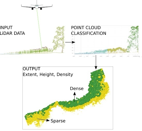
1. Introduction
- How accurate is the estimation of aquatic reed extent in LiDAR point clouds?
- How accurate is the estimation of aquatic reed density in LiDAR point clouds?
- How accurately can aquatic reed bed DSMs be calculated from LiDAR point clouds?
2. Material and Methods
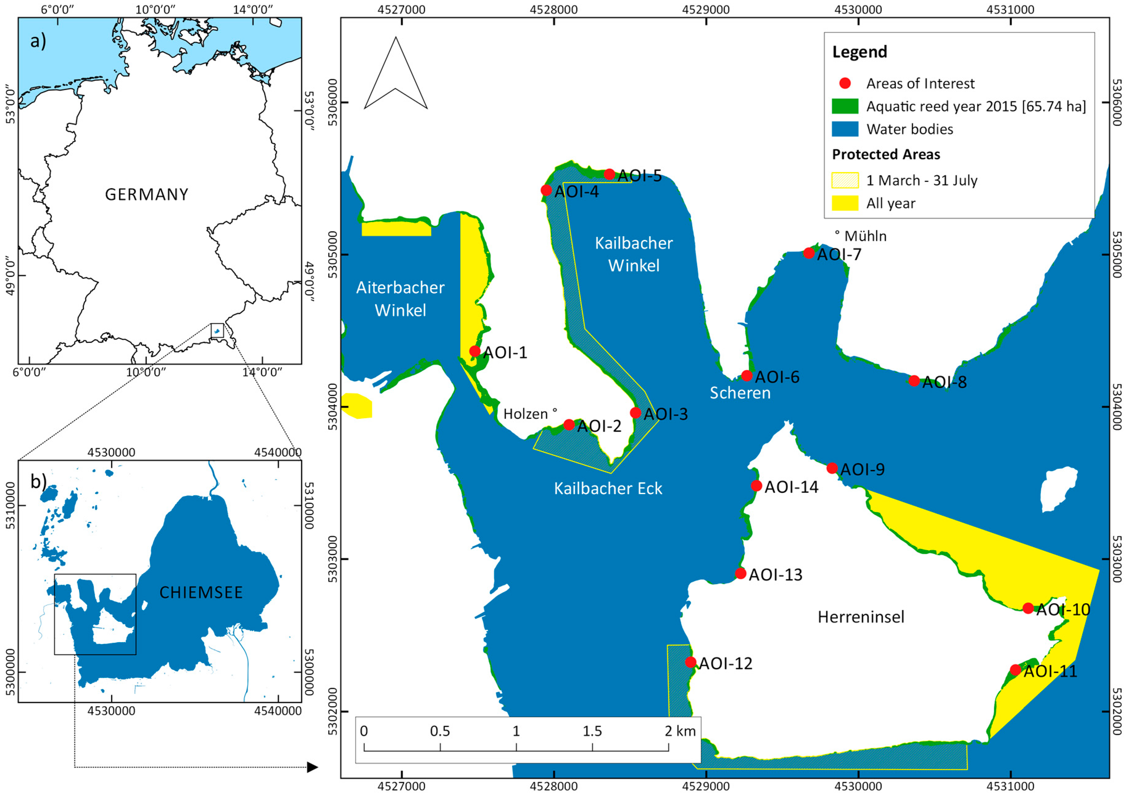
2.1. Study Area
2.2. Airborne Laser Scanning Processing Chain
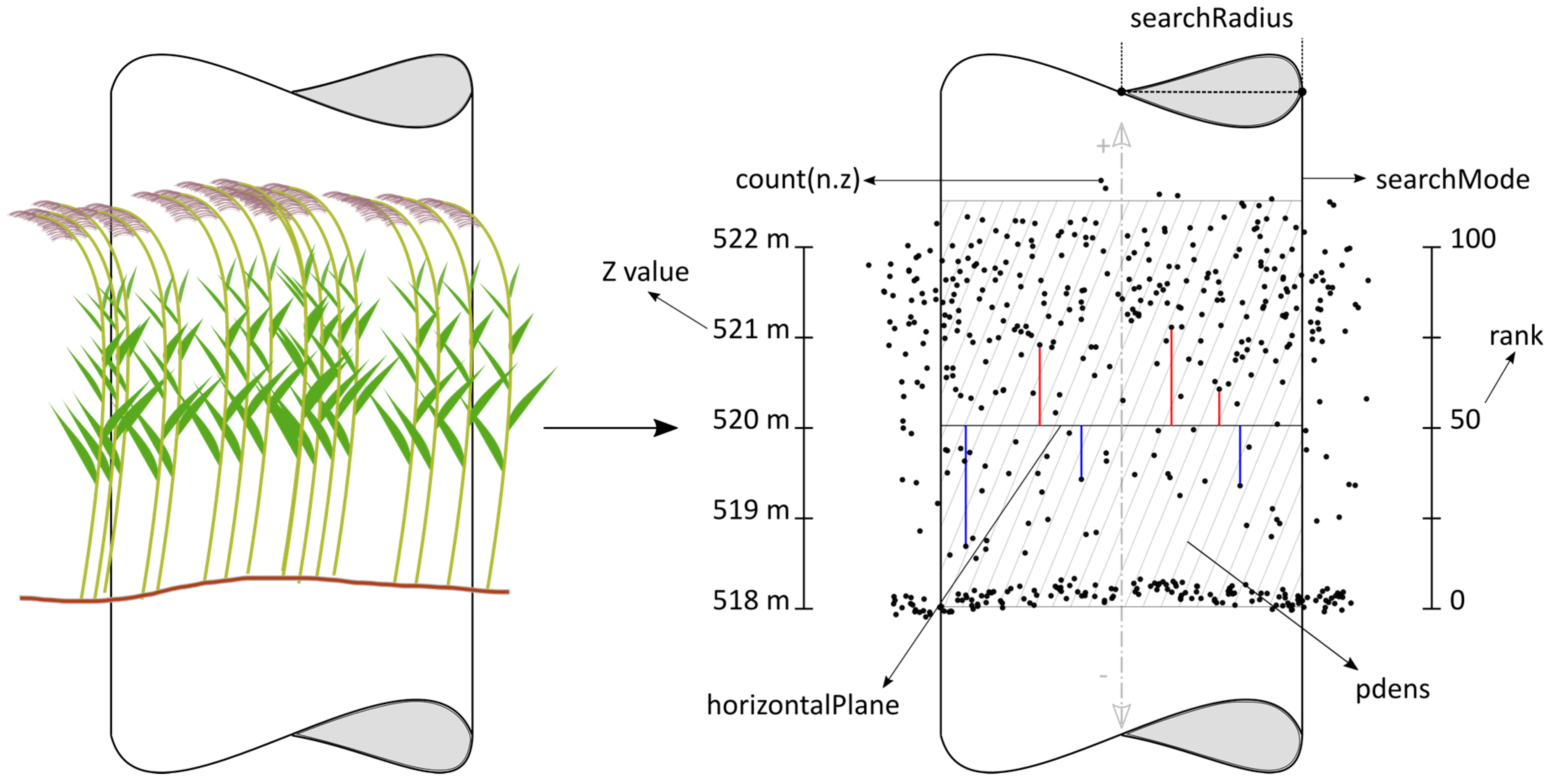
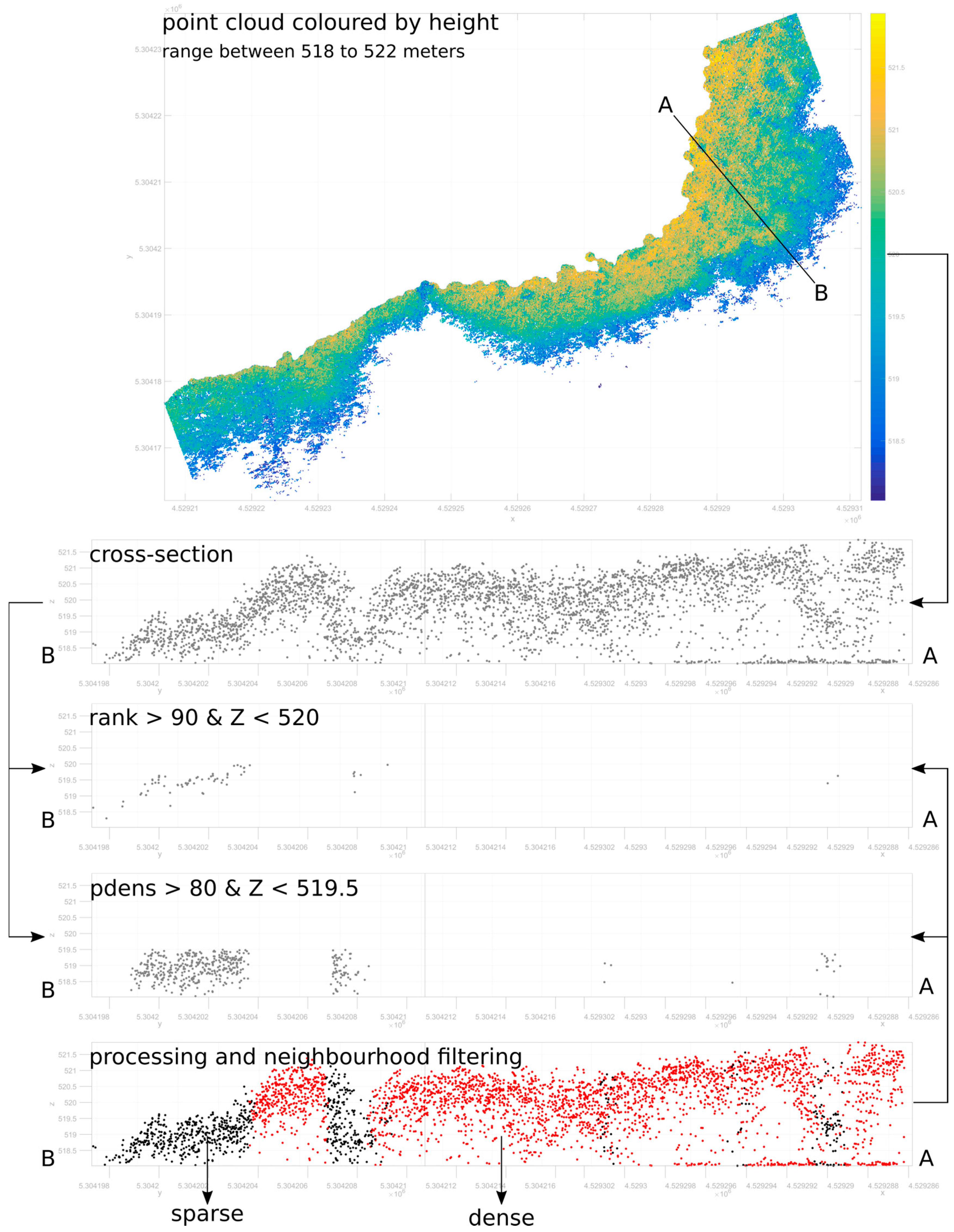
2.2.1. Classification of Green-LiDAR Data
2.2.2. Validation Data
2.2.3. Assessment of Aquatic Reed Extents and Classification Accuracy
2.2.4. Accuracy Assessment of DSM
3. Results
3.1. Point Cloud Classification
3.2. Assessment of Aquatic Reed Bed Extents
3.3. Assessment of Aquatic Reed Bed Densities
3.4. Accuracy Assessment for Calculated DSM of Aquatic Reed Beds
4. Discussion
4.1. Mapping On-Field Concept and Extent Quantification
4.2. Classification of Aquatic Reed Bed Density
4.3. Reed Heights Measured on DSM
4.4. LiDAR Processing Chain and ALS Data Collection
5. Conclusions
Acknowledgments
Author Contributions
Conflicts of Interest
References
- Ostendorp, W. Schilf als Lebensraum. In Beihefte zu den Veröffentlichungen für Naturschutz und Landschaftspflege in Baden-Württemberg; Landesanst. für Umweltschutz Baden-Württemberg: Karlsruhe, Germany, 1993; Volume 68. [Google Scholar]
- Grosser, S.; Pohl, W.; Melzer, A. Untersuchung des Schilfrückgangs an bayerischen Seen: Forschungsprojekt des Bayerischen Staatsministeriums für Landesentwicklung und Umweltfragen; LfU: München, Germany, 1997. [Google Scholar]
- Ostendorp, W.; Dienst, M.; Schmieder, K. Disturbance and rehabilitation of lakeside Phragmites reeds following an extreme flood in Lake Constance (Germany). Hydrobiologia 2003, 506–509, 687–695. [Google Scholar] [CrossRef]
- Crisman, T.L.; Alexandridis, T.K.; Zalidis, G.C.; Takavakoglou, V. Phragmites distribution relative to progressive water level decline in Lake Koronia, Greece. Ecohydrology 2014, 7, 1403–1411. [Google Scholar] [CrossRef]
- Nechwatal, J.; Wielgoss, A.; Mendgen, K. Flooding events and rising water temperatures increase the significance of the reed pathogen Pythium phragmitis as a contributing factor in the decline of Phragmites australis. Hydrobiologia 2008, 613, 109–115. [Google Scholar] [CrossRef]
- Schmieder, K.; Dienst, M.; Ostendorp, W.; Jöhnk, K. Effects of water level variations on the dynamics of the reed belts of Lake Constance. Ecohydrol. Hydrobiol. 2004, 4, 469–480. [Google Scholar]
- Schmieder, K.; Dienst, M.; Ostendorp, W. Auswirkungen des Extremhochwassers 1999 auf die Flächendynamik und Bestandsstruktur der Uferröhrichte des Bodensees. Limnol.—Ecol. Manag. Inland Waters 2002, 32, 131–146. [Google Scholar] [CrossRef]
- Ostendorp, W.; Tiedge, E.; Hille, S. Effect of eutrophication on culm architecture of lakeshore Phragmites reeds. Aquat. Bot. 2001, 69, 177–193. [Google Scholar] [CrossRef]
- Ostendorp, W. ‘Die-back’ of reeds in Europe—A critical review of literature. Aquat. Bot. 1989, 35, 5–26. [Google Scholar] [CrossRef]
- Gigante, D.; Venanzoni, R.; Zuccarello, V. Reed die-back in southern Europe? A case study from Central Italy. C. R. Biol. 2011, 334, 327–336. [Google Scholar] [CrossRef] [PubMed]
- Tóth, V.R. Reed stands during different water level periods: Physico-chemical properties of the sediment and growth of Phragmites australis of Lake Balaton. Hydrobiologia 2016, 778, 193–207. [Google Scholar] [CrossRef]
- Schmieder, K.; Woithon, A. Einsatzt von Fernerkundung im Rahmen aktueller Forschungsprojekte zur Gewässerökologie an der Universität Hohenheim. In Erfassung und Beurteilung von Seen und Deren Einzugsgebieten mit Methoden der Fernerkundung: Tagungsband der ANL-Fachveranstaltung vom 11. bis 12. September in Laufen; Obermaier, E., Ed.; Bayerische Akademie für Naturschutz und Landschaftspflege (ANL): Laufen, Switzerland, 2004; Volume 2003, pp. 39–45. [Google Scholar]
- Krumscheid, P.; Stark, H.; Peintinger, M. Decline of reed at Lake Constance (Obersee) since 1967 based on interpretations of aerial photographs. Aquat. Bot. 1989, 35, 57–62. [Google Scholar] [CrossRef]
- Kristiansen, J.N.; Petersen, B.M. Remote sensing as a technique to asses reedbed suitability for nesting Greylag geese Anser anser. Ardea 2000, 88, 253–257. [Google Scholar]
- Dienst, M.; Schmieder, K.; Ostendorp, W. Dynamik der Schilfröhrichte am Bodensee unter dem Einfluss von Wasserstandsvariationen. Limnol.—Ecol. Manag. Inland Waters 2004, 34, 29–36. [Google Scholar] [CrossRef]
- Davranche, A.; Lefebvre, G.; Poulin, B. Wetland monitoring using classification trees and SPOT-5 seasonal time series. Remote Sens. Environ. 2010, 114, 552–562. [Google Scholar] [CrossRef]
- Villa, P.; Laini, A.; Bresciani, M.; Bolpagni, R. A remote sensing approach to monitor the conservation status of lacustrine Phragmites australis beds. Wetl. Ecol. Manag. 2013, 21, 399–416. [Google Scholar] [CrossRef]
- Brix, H.; Ye, S.; Laws, E.A.; Sun, D.; Li, G.; Ding, X.; Yuan, H.; Zhao, G.; Wang, J.; Pei, S. Large-scale management of common reed, Phragmitesaustralis, for paper production: A case study from the Liaohe Delta, China. Ecol. Eng. 2014, 73, 760–769. [Google Scholar] [CrossRef]
- Bourgeau-Chavez, L.; Endres, S.; Battaglia, M.; Miller, M.E.; Banda, E.; Laubach, Z.; Higman, P.; Chow-Fraser, P.; Marcaccio, J. Development of a bi-national Great Lakes coastal wetland and land use map using three-season PALSAR and Landsat imagery. Remote Sens. 2015, 7, 8655–8682. [Google Scholar] [CrossRef]
- Melzer, A.; Zimmermann, S.; Wissen, U. Maßnahmenplanung zur Entwicklung der Aquatischen Röhrichte am Starnberger See; Wasserwirtschaftsamt München: München, Germany, 2001. [Google Scholar]
- Hoffmann, F.; Zimmermann, S. Chiemsee Schilfkataster: 1973, 1979, 1991 und 1998; Wasserwirtschaftsamt Traunstein: Traunstein, Germany, 2000. [Google Scholar]
- Venturi, S.; Di Francesco, S.; Materazzi, F.; Manciola, P. Unmanned aerial vehicles and Geographical Information System integrated analysis of vegetation in Trasimeno Lake, Italy. Lakes Reserv. Res. Manag. 2016, 21, 5–19. [Google Scholar] [CrossRef]
- Luo, S.; Wang, C.; Xi, X.; Pan, F.; Qian, M.; Peng, D.; Nie, S.; Qin, H.; Lin, Y. Retrieving aboveground biomass of wetland Phragmites australis (common reed) using a combination of airborne discrete-return LiDAR and hyperspectral data. Int. J. Appl. Earth Obs. Geoinf. 2017, 58, 107–117. [Google Scholar] [CrossRef]
- Zlinszky, A.; Mücke, W.; Lehner, H.; Briese, C.; Pfeifer, N. Categorizing wetland vegetation by airborne laser scanning on Lake Balaton and Kis-Balaton, Hungary. Remote Sens. 2012, 4, 1617–1650. [Google Scholar] [CrossRef]
- Onojeghuo, A.O.; Blackburn, G.A. Optimising the use of hyperspectral and LiDAR data for mapping reedbed habitats. Remote Sens. Environ. 2011, 115, 2025–2034. [Google Scholar] [CrossRef]
- Gilmore, M.S.; Wilson, E.H.; Barrett, N.; Civco, D.L.; Prisloe, S.; Hurd, J.D.; Chadwick, C. Integrating multi-temporal spectral and structural information to map wetland vegetation in a lower Connecticut River tidal marsh. Remote Sens. Environ. 2008, 112, 4048–4060. [Google Scholar] [CrossRef]
- Onojeghuo, A.O.; Blackburn, G.A.; Latif, Z.A. (Eds.) Characterising Reedbed Habitat Quality Using Leaf-Off LiDAR Data: 21–23 May 2010, Mahkota Hotel, Melaka, Malaysia; Proceedings; IEEE: Piscataway, NJ, USA, 2010. [Google Scholar]
- Mandlburger, G.; Pfennigbauer, M.; Pfeifer, N. Analyzing near water surface penetration in laser bathymetry—A case study at the River Pielach. ISPRS Ann. Photogramm. Remote Sens. Spat. Inf. Sci. 2013, II-5/W2, 175–180. [Google Scholar] [CrossRef]
- Costa, B.M.; Battista, T.A.; Pittman, S.J. Comparative evaluation of airborne LiDAR and ship-based multibeam SoNAR bathymetry and intensity for mapping coral reef ecosystems. Remote Sens. Environ. 2009, 113, 1082–1100. [Google Scholar] [CrossRef]
- Wedding, L.M.; Friedlander, A.M.; McGranaghan, M.; Yost, R.S.; Monaco, M.E. Using bathymetric lidar to define nearshore benthic habitat complexity: Implications for management of reef fish assemblages in Hawaii. Remote Sens. Environ. 2008, 112, 4159–4165. [Google Scholar] [CrossRef]
- Tulldahl, H.M.; Wikström, S.A. Classification of aquatic macrovegetation and substrates with airborne lidar. Remote Sens. Environ. 2012, 121, 347–357. [Google Scholar] [CrossRef]
- Mandlburger, G.; Hauer, C.; Wieser, M.; Pfeifer, N. Topo-Bathymetric LiDAR for Monitoring River Morphodynamics and Instream Habitats: A Case Study at the Pielach River. Remote Sens. 2015, 7, 6160–6195. [Google Scholar] [CrossRef]
- Yamamoto, K.H.; Powell, R.L.; Anderson, S.; Sutton, P.C. Using LiDAR to quantify topographic and bathymetric details for sea turtle nesting beaches in Florida. Remote Sens. Environ. 2012, 125, 125–133. [Google Scholar] [CrossRef]
- Bayerisches Landesamt für Umwelt. Seen in Bayern—LfU Bayern 2017. Available online: https://www.lfu.bayern.de/wasser/seen_in_bayern/index.htm (accessed on 23 May 2017).
- Pfeifer, N.; Mandlburger, G.; Otepka, J.; Karel, W. OPALS—A framework for Airborne Laser Scanning data analysis. Comput. Environ. Urban Syst. 2014, 45, 125–136. [Google Scholar] [CrossRef]
- Smith, M.; Vericat, D.; Gibbins, C. Through-water terrestrial laser scanning of gravel beds at the patch scale. Earth Surf. Process. Landf. 2012, 37, 411–421. [Google Scholar] [CrossRef]
- Bayerisches Landesamt für Umwelt. Gewässerkundlicher Dienst Bayern 2017. Available online: https://www.gkd.bayern.de/ (accessed on 1 June 2017).
- QGIS Development Team. QGIS Geographic Information System. Available online: https://www.qgis.org/en/site/ (accessed on 1 June 2017).
- Congalton, R.G.; Green, K. Assessing the Accuracy of Remotely Sensed Data: Principles and Practices, 2nd ed.; CRC Press/Taylor & Francis: Boca Raton, FL, USA, 2009. [Google Scholar]
- Richards, J.A.; Jia, X. Remote Sensing Digital Image Analysis: An Introduction, 4th ed.; Springer: Berlin, Germany; New York, NY, USA, 2006. [Google Scholar]
- Lillesand, T.M.; Kiefer, R.W.; Chipman, J.W. Remote Sensing and Image Interpretation, 7th ed.; John Wiley: Hoboken, NJ, USA, 2015. [Google Scholar]
- Höhle, J.; Höhle, M. Accuracy assessment of digital elevation models by means of robust statistical methods. ISPRS J. Photogram. Remote Sens. 2009, 64, 398–406. [Google Scholar] [CrossRef]
- Luhmann, T.; Kyle, S.; Böhm, J.; Robson, S. (Eds.) Close-Range Photogrammetry and 3D Imaging, 2nd ed.; De Gruyter: Berlin, Germany, 2014. [Google Scholar]
- Stratoulias, D.; Balzter, H.; Sykioti, O.; Zlinszky, A.; Toth, V.R. Evaluating Sentinel-2 for Lakeshore Habitat Mapping Based on Airborne Hyperspectral Data. Sensors 2015, 15, 22956–22969. [Google Scholar] [CrossRef] [PubMed]
- Fernandes, M.R.; Aguiar, F.C.; Silva, J.M.; Ferreira, M.T.; Pereira, J.M. Optimal attributes for the object based detection of giant reed in riparian habitats: A comparative study between Airborne High Spatial Resolution and WorldView-2 imagery. Int. J. Appl. Earth Obs. Geoinf. 2014, 32, 79–91. [Google Scholar] [CrossRef]


| Class | Area (m2) | Area (ha) | Number of Samples |
|---|---|---|---|
| Sparse Aquatic Reed | 4843 | 0.4843 | 50 |
| Dense Aquatic Reed | 9037 | 0.9037 | 100 |
| Mean Error | [42] | |
| Standard Deviation | [42] | |
| Root Mean Square Error | [42,43] |
| Reference Data | Reference Data | ||||||||
|---|---|---|---|---|---|---|---|---|---|
| Classified Data | Dense | Sparse | Total | User’s Accuracy (%) | Classified Data | Dense | Sparse | Total | User’s Accuracy(%) |
| Dense | 74 | 18 | 92 | 80.4 | Dense | 47 | 3 | 50 | 94 |
| Sparse | 50 | 1.07 | 157 | 68.2 | Sparse | 3 | 97 | 100 | 97 |
| Total | 124 | 125 | 249 | Total | 50 | 100 | 50 | ||
| Producer’s Accuracy (%) | 59.7 | 85.6 | Producer’s Accuracy (%) | 94 | 97 | 150 | |||
| Overall Accuracy (%) = 72.7; Kappa = 0.5 | Overall Accuracy (%) = 96; Kappa = 0.91 | ||||||||
© 2017 by the authors. Licensee MDPI, Basel, Switzerland. This article is an open access article distributed under the terms and conditions of the Creative Commons Attribution (CC BY) license (http://creativecommons.org/licenses/by/4.0/).
Share and Cite
Corti Meneses, N.; Baier, S.; Geist, J.; Schneider, T. Evaluation of Green-LiDAR Data for Mapping Extent, Density and Height of Aquatic Reed Beds at Lake Chiemsee, Bavaria—Germany. Remote Sens. 2017, 9, 1308. https://doi.org/10.3390/rs9121308
Corti Meneses N, Baier S, Geist J, Schneider T. Evaluation of Green-LiDAR Data for Mapping Extent, Density and Height of Aquatic Reed Beds at Lake Chiemsee, Bavaria—Germany. Remote Sensing. 2017; 9(12):1308. https://doi.org/10.3390/rs9121308
Chicago/Turabian StyleCorti Meneses, Nicolás, Simon Baier, Juergen Geist, and Thomas Schneider. 2017. "Evaluation of Green-LiDAR Data for Mapping Extent, Density and Height of Aquatic Reed Beds at Lake Chiemsee, Bavaria—Germany" Remote Sensing 9, no. 12: 1308. https://doi.org/10.3390/rs9121308
APA StyleCorti Meneses, N., Baier, S., Geist, J., & Schneider, T. (2017). Evaluation of Green-LiDAR Data for Mapping Extent, Density and Height of Aquatic Reed Beds at Lake Chiemsee, Bavaria—Germany. Remote Sensing, 9(12), 1308. https://doi.org/10.3390/rs9121308