Article

An Evaluation of Satellite Estimates of Solar Surface Irradiance Using Ground Observations in San Antonio, Texas, USA

1
Texas Sustainable Energy Research Institute, University of Texas at San Antonio, San Antonio, TX 78249, USA
2
Laboratory for Remote Sensing and Geoinformatics, Department of Geological Sciences, University of Texas at San Antonio, San Antonio, TX 78249, USA
3
CPS Energy, San Antonio, TX 78205, USA
*
Author to whom correspondence should be addressed.
Remote Sens. 2017, 9(12), 1268; https://doi.org/10.3390/rs9121268
Submission received: 27 October 2017 / Revised: 23 November 2017 / Accepted: 4 December 2017 / Published: 7 December 2017
(This article belongs to the Section Biogeosciences Remote Sensing)

Abstract

:
Estimates of solar irradiance at the earth’s surface from satellite observations are useful for planning both the deployment of distributed photovoltaic systems and their integration into electricity grids. In order to use surface solar irradiance from satellites for these purposes, validation of its accuracy against ground observations is needed. In this study, satellite estimates of surface solar irradiance from Geostationary Operational Environmental Satellite (GOES) are compared with ground observations at two sites, namely the main campus of the University of Texas at San Antonio (UTSA) and the Alamo Solar Farm of San Antonio (ASF). The comparisons are done mostly on an hourly timescale, under different cloud conditions classified by cloud types and cloud layers, and at different solar zenith angle intervals. It is found that satellite estimates and ground observations of surface solar irradiance are significantly correlated (p < 0.05) under all sky conditions (r: 0.80 and 0.87 on an hourly timescale and 0.94 and 0.91 on a daily timescale, respectively for the UTSA and ASF sites); on the hourly timescale, the correlations are 0.77 and 0.86 under clear-sky conditions, and 0.74 and 0.84 under cloudy conditions, respectively for the UTSA and ASF sites, and mostly >0.60 under different cloud types and layers for both sites. The correlations under cloudy-sky conditions are mostly stronger than those under clear-sky conditions at different solar zenith angles. The correlation coefficients are mostly the smallest with solar zenith angle in the range of 75–90° under all sky, clear-sky and cloudy-sky conditions. At the ASF site, the overall bias of GOES surface solar irradiance is small (+1.77 Wm−2) under all sky while relatively larger under clear-sky (−22.29 Wm−2) and cloudy-sky (+40.31 Wm−2) conditions. The overall good agreement of the satellite estimates with the ground observations underscores the usefulness of the GOES surface solar irradiance estimates for solar energy studies in the San Antonio area.

Graphical Abstract

1. Introduction

Solar irradiance is the solar power per unit area (Wm−2) received from the Sun in the form of shortwave electromagnetic radiation. Because it is an abundant source of green energy, solar irradiance has a great potential for various types of applications in the near future including water treatment plants [1,2], water supply and sanitation [3,4], environmental protection [5,6,7], and as an alternative to fossil fuel energy generation [8,9]. For developing these applications, worldwide accurate measurement of solar irradiance and of its variability over space and time are needed. Due to its global coverage, satellite estimates of solar irradiance offer obvious advantages over in situ measurements. Nevertheless, the quality of satellite estimates still need to be ground-truthed with direct in situ measurements.
Since January 1996, the National Oceanic and Atmospheric Administration (NOAA)/National Environmental Satellite, Data, and Information Service (NESDIS) has retrieved parameters for evaluating the surface shortwave radiation balance from the Geostationary Operational Environmental Satellite system (GOES) in real time [10,11]. These satellite observations have allowed the implementation of radiative transfer models for solar radiation. Validation of the GOES-derived satellite surface solar irradiance (Gs), estimated from these types of models, with ground measured global horizontal irradiance (Gg) has been conducted by many previous studies [12,13,14,15,16,17,18]. For example, Pinker et al. [13] compared Gs, retrieved from the GOES Surface and Insolation Products (GSIP), and Gg from about 50 stations and found the correlation coefficients between them on different timescales were all greater than 0.90, with a bias and RMSE (root mean squared error) of −36–5 Wm−2 and 87–104 Wm−2 on an hourly timescale, −11–8 Wm−2 and 22–29 Wm−2 on a daily timescale, and −11–8 Wm−2 and 14–19 Wm−2 on a monthly timescale, respectively. Otkin et al. [16] found that the correlation coefficient for the seasonal comparison of Gs retrieved from a physical model and Gg on different timescales at 11 sites was also high (0.95), with a bias of 8 Wm−2 (GOES_E) and −9 Wm−2 (GOES_W) and RMSE of 63 Wm−2 on an hourly timescale, and the bias of 4 Wm−2 (GOES_E) and −17 Wm−2 (GOES_W) and RMSE of 16 Wm−2 on the daily timescale.
All the above-mentioned studies have showed that there is overall good agreements between Gs and Gg under all sky conditions, with RMSE and bias mostly in the ranges of 63–104 Wm−2 and −36–5 Wm−2 on an hourly timescale and 15–49 Wm−2 and −11–8 Wm−2 on a daily timescale, respectively. None of the cited studies, however, has examined the cloud effect on the surface solar irradiance mapping from GOES satellites. The only study that considered the cloud effect was the one by Habte et al. [17] that compared Gs and Gg under clear-sky and cloudy-sky conditions on an hourly timescale and found (1) better correlation under clear-sky conditions than that under cloudy-sky conditions and (2) that Gs is biased higher (overestimation) under clear-sky conditions than under cloudy-sky conditions, especially at low solar zenith angles.
Although many factors (such as aerosol, water vapor and ozone) could attenuate the solar radiation reaching the Earth’s surface, clouds are considered as the primary effect [19,20,21] and their attenuation is much larger than that of the atmosphere. Therefore, the objective of this work is to explore the correlation between Gs and Gg on hourly (and daily) timescales, under different cloud conditions in terms of cloud types and cloud layers, and at different solar zenith angle intervals. The ultimate goal is to determine if real time satellite estimates are reliable and acceptable for future solar forecasting and mapping.

2. Data

The radiation hitting the surface of the earth can be represented in a number of different ways. In this paper, we focus on global horizontal irradiance (G) which is the amount of shortwave radiation received from above (downwelling) by a surface horizontal to the ground and includes both direct normal irradiance and diffuse horizontal irradiance. The observational data of G comes from satellite estimates (Gs) and ground direct measurements (Gg).

2.1. Satellite Estimates

For GSIP, the physical radiative transfer model of Pinker and Ewing [12] was modified and expanded by Pinker and Laszlo [22,23] to derive estimates of Gs in the 0.2–4.0 μm spectral range from GOES satellite observations. Reflectivity (R), transmissivity (T), and absorptivity of the atmosphere can be determined, respectively, by optical depth, single-scattering albedo, and phase function/asymmetry parameter recovered from geostationary satellite data. The method is based on relating T to R, which describe the radiative state of the atmosphere and that of the surface. Once the relationship T = f(R) is known, T can be determined from satellite observations of top-of-the-atmosphere (TOA) reflectivity R. The downwelling radiation at the Earth’s surface can be computed if T is known. This model accounts for solar zenith angle, absorption by ozone and water vapor, multiple scattering by molecules, multiple scattering and absorption by aerosols and cloud droplets and multiple reflection between the atmosphere and the surface. The information of these input atmosphere and surface parameters are from the NOAA National Centers for Environmental Prediction (NCEP) at NESDIS in real time [24,25,26,27]. The surface albedo is calculated from the observed “clearest” shortwave TOA albedo over a number of days and then corrected for Rayleigh scattering, aerosol extinction, and absorption by ozone and water vapor. The aerosols come from Standard Radiation Atmospheres, clouds from Stephens et al. [28], ozone is obtained from the McClatchy atmospheres, and water vapor from the NCEP Eta model. A large number of radiative transfer computations should be conducted to determine T = f(R) for all possible realistic combinations of all parameters [22,23]. These computations applied to GOES were described in detail in Pinker et al. [10,13]. Laszlo et al. [11] gave an overview of remote sensing of shortwave radiation budget retrieved from the GOES series. Satellite solar irradiance (Gs) at the earth’s surface is related to that at the top of the atmosphere (Gtop) as follows:
Gs = T × Gtop,
where T is primarily determined by the composition of the atmosphere, the length of the path that solar radiation travels through the atmosphere, and the albedo of the Earth’s surface [13].
The Gs, cloud type, and cloud layer data used in this study come from the NOAA GOES Surface and Insolation Products (GSIP) based on the visible and infrared channels of GOES satellites (GOES East and GOES West), 45 min after the hour and on the hour during daytime [29]. The identification of cloud types and layers (Table 1) is based on the work of Pavolonis et al. [30]. The resolution of the GSIP products in San Antonio is about 2.3 km in longitude × 4.9 km in latitude (i.e., about 11 km2).

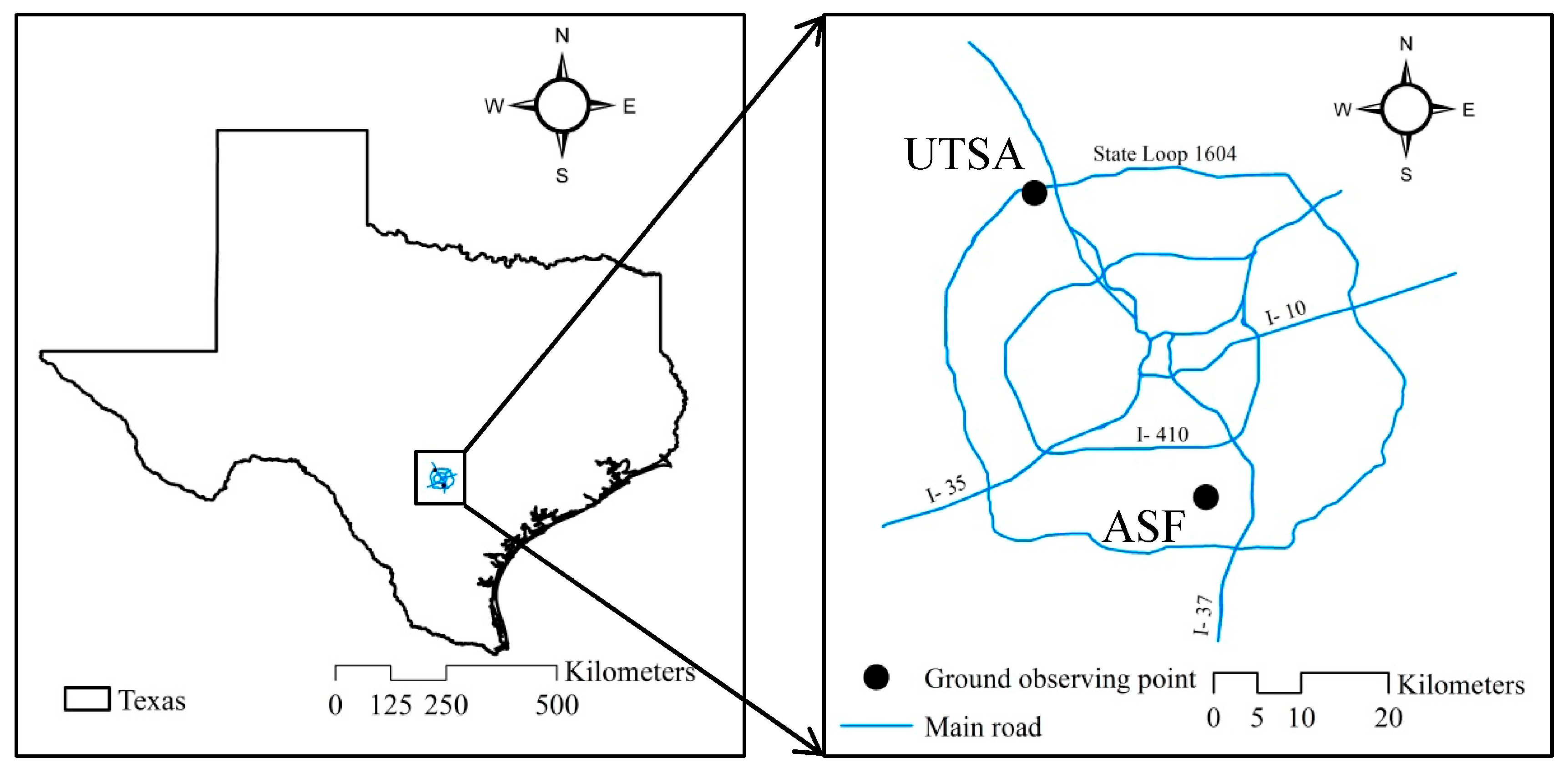
2.2. Ground Observations

In situ measurements of Gg at the main campus of the University of Texas at San Antonio (UTSA) and the Alamo Solar Farm of San Antonio (ASF), Texas (Figure 1) are used to compare with Gs. At the UTSA site (29.5833°N, 98.6199°W), Gg was recorded at 5 min resolution from 1 May to 25 October 2015 by a horizontally installed LI-200R pyranometer with a typical uncertainty of 3%, including direct and diffuse solar radiation in the 0.4–1.1 µm spectral range. At the ASF site (29.7010°N, 98.4432°W), Gg was recorded at irregular time intervals with a sampling distribution having a mean of 0.16 min and standard deviation of 0.23 min from 1 July to 30 September 2014 and 22 September, 2015 to 18 October 2016. The instrument used was a horizontally installed CMP11_L pyranometer with an uncertainty of <2% and spectral range of 0.285–2.8 µm. The number of observations is 3265 and 9840 for the UTSA and ASF sites, respectively. The sampling intervals of both ground-based pyranometers are thus significantly finer than that of the satellite’s sensor. The accuracy of the radiative model and pyranometers degrades rapidly at larger zenith angles, especially near the horizon [32].

3. Method

Comparisons between collocated estimates of Gs and Gg are performed on hourly and daily timescales, for clear-sky and cloudy sky conditions, and at different solar zenith angles. The statistical measures used to describe comparisons are correlation coefficient (r), simple differences (e), bias, root mean square error (RMSE), and relative RMSE in percentage (%RMSE) as follows
e = Gs − Gg
b i a s = e n
R M S E = ( e 2 ) n
% R M S E = R M S E G g n × 100
where Gs and Gg denote the satellite estimates and ground measurements of G, respectively, and n is the number of collocated samples, following Mellit and Pavan [33] and Lave et al. [29].

4. Results

4.1. Descriptive Statistics of Cloud Occurrence and Surface Solar Irradiance

Table 2 shows the number of observations and percentage of occurrences for various sky conditions (clear, partly cloudy, water, mixed, glaciated, cirrus, and multilayered) in three layers classified by altitude (low, mid and high) at UTSA and ASF sites. Overall, the clear-sky condition is the most frequent sky condition at both sites (~66% and ~62%, respectively), followed by water clouds (~13% and ~14%) and cirrus clouds (~12% and ~15%). At the low cloud layer, water clouds occur most frequently (~7% and ~10%). At the mid cloud layer, both water (~5% and ~4%) and cirrus clouds (~4% and ~5%) are the most frequently occurring. At the high cloud layer, cirrus clouds lead the frequency of occurrence at both sites (~6% and ~7%).
Figure 2 shows mean hourly surface solar irradiance (Gs and Gg) at both sites for both clear-sky and cloudy-sky conditions. Under clear-sky conditions, it is found that Gs is larger than Gg at the UTSA site but the opposite is generally true at the ASF site. It is also found that Gs and Gg increase with decreasing solar zenith angle (before solar noon) and decrease with increasing solar zenith angle (after solar noon), at both sites. As expected, G for clear-sky conditions is higher than that for any cloudy condition and depends only on aerosol optical depth, amount of water vapor, amount of ozone, illumination geometry, and surface albedo.
Under cloudy-sky conditions, G is high with water clouds, followed by mixed-phase and cirrus clouds at both sites. For most cloud types, Gs is larger than Gg at both sites. Partly cloudy mainly occurs at the low layer and is thicker than high clouds, thus reflecting more radiation back to space. Water clouds are composed of liquid water drops. They are the dominant absorbers of infrared radiation [34,35]. It is the same for mixed phase clouds, which is composed of supercooled water droplets or both ice and supercooled water [36]. Both the Gs and Gg are low for glaciated clouds. It is because glaciated clouds are entirely composed of ice crystals or opaque clouds with glaciated tops that are constantly with deep convection [37]. They are non-transmissive clouds thus they do not allow as much solar energy to reach the earth’s surface. Instead, they reflect much of the solar energy back to space [38]. It is the same for multilayered clouds. Cirrus clouds are high, thin clouds. They act in a similar way to clear sky because they are highly transparent to shortwave radiation, therefore Gs and Gg under cirrus clouds are relatively high [39].

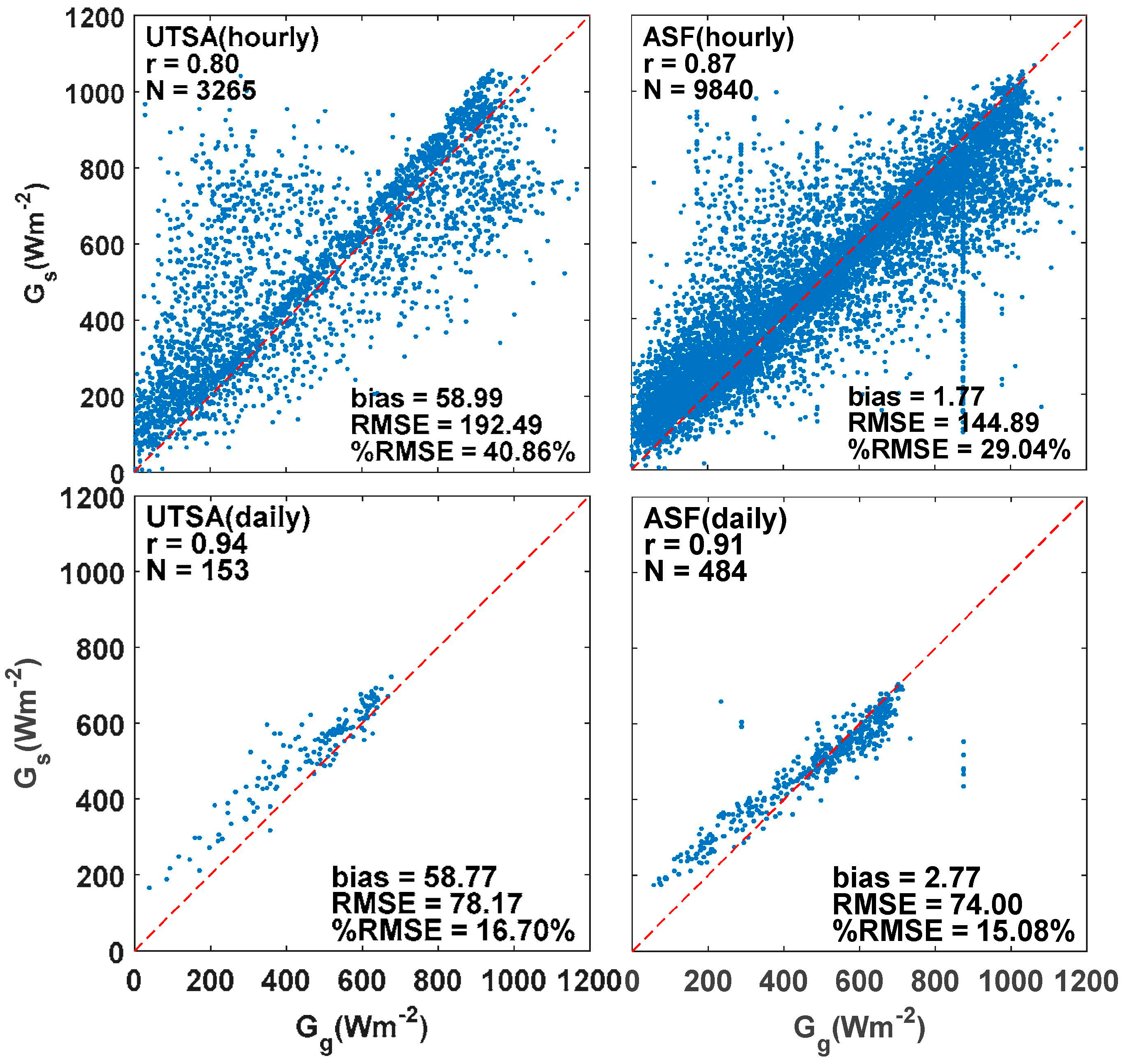
4.2. Comparison of Gs and Gg on Hourly and Daily Timescales under All Sky Conditions

Comparisons of Gs derived from GOES East and GOES West imagery with Gg from the two sites at hourly and daily timescales are presented in Figure 3. On an hourly timescale, the correlation coefficients between Gs and Gg are 0.80 and 0.87, with biases of 58.99 and 1.77 Wm−2, RMSE of 192.49 and 144.89 Wm−2, and %RMSE of 40.86% and 29.04%, at UTSA and ASF, respectively. On a daily timescale, the correlation coefficients between Gs and Gg are 0.94 and 0.91 with slightly reduced biases of 58.77 and 2.77 Wm−2, significantly reduced RMSE of 78.17 and 74.00 Wm−2, and reduced %RMSE of 16.70% and 15.08% at the two sites, all better than those on the hourly scale. This means that daily averaging could reduce the biases and cancel out the random errors which could contribute to the discrepancies, as compared with those on the hourly timescale. Absolute values of bias, RMSE and %RMSE are lower at the ASF site than those at the UTSA site. Overall, as compared with Gg, satellite-derived Gs tends to be higher when G is low and lower when G is high.

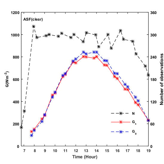
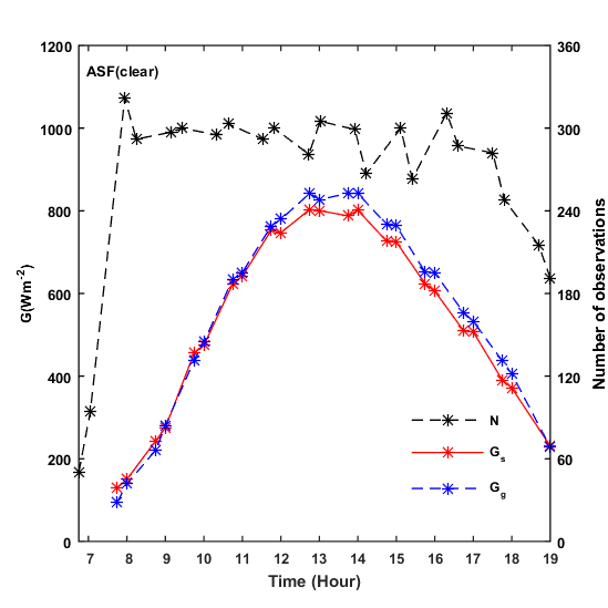
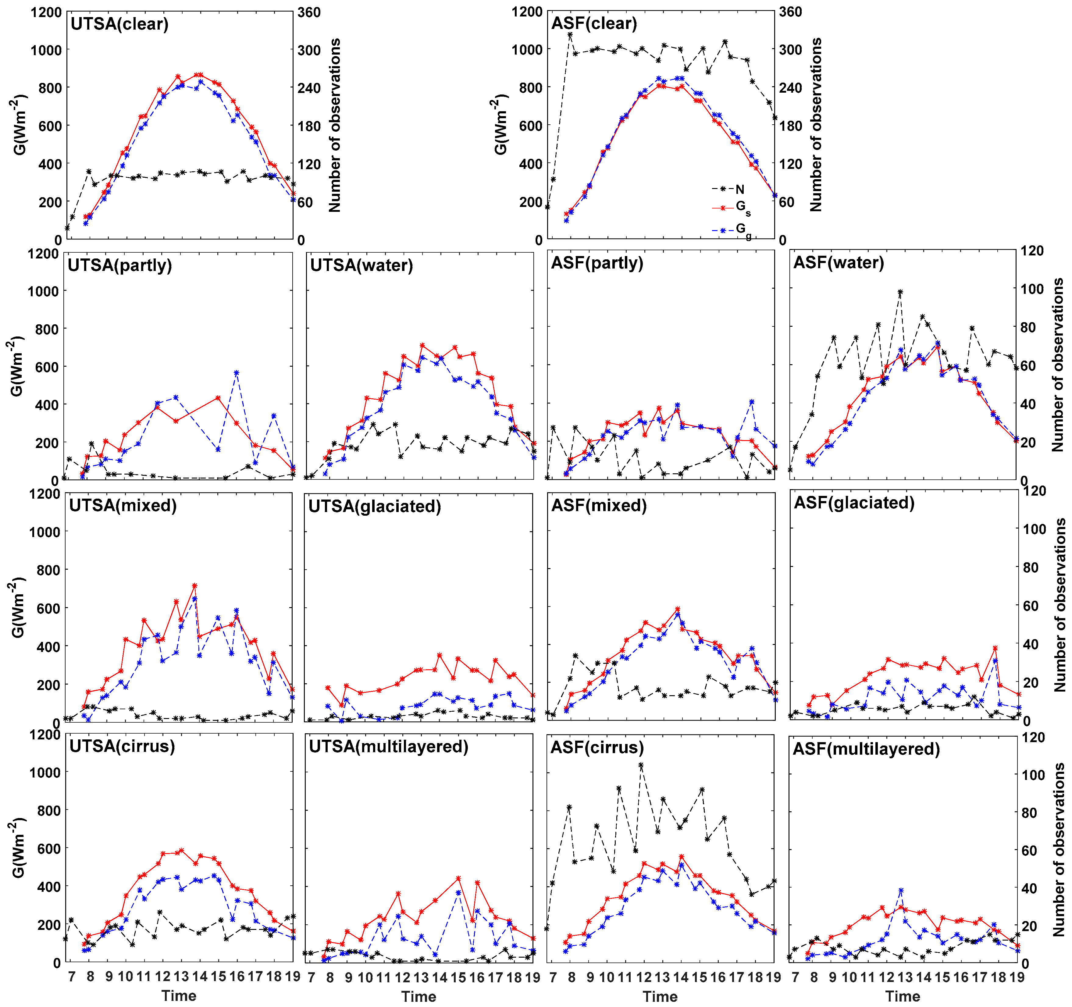
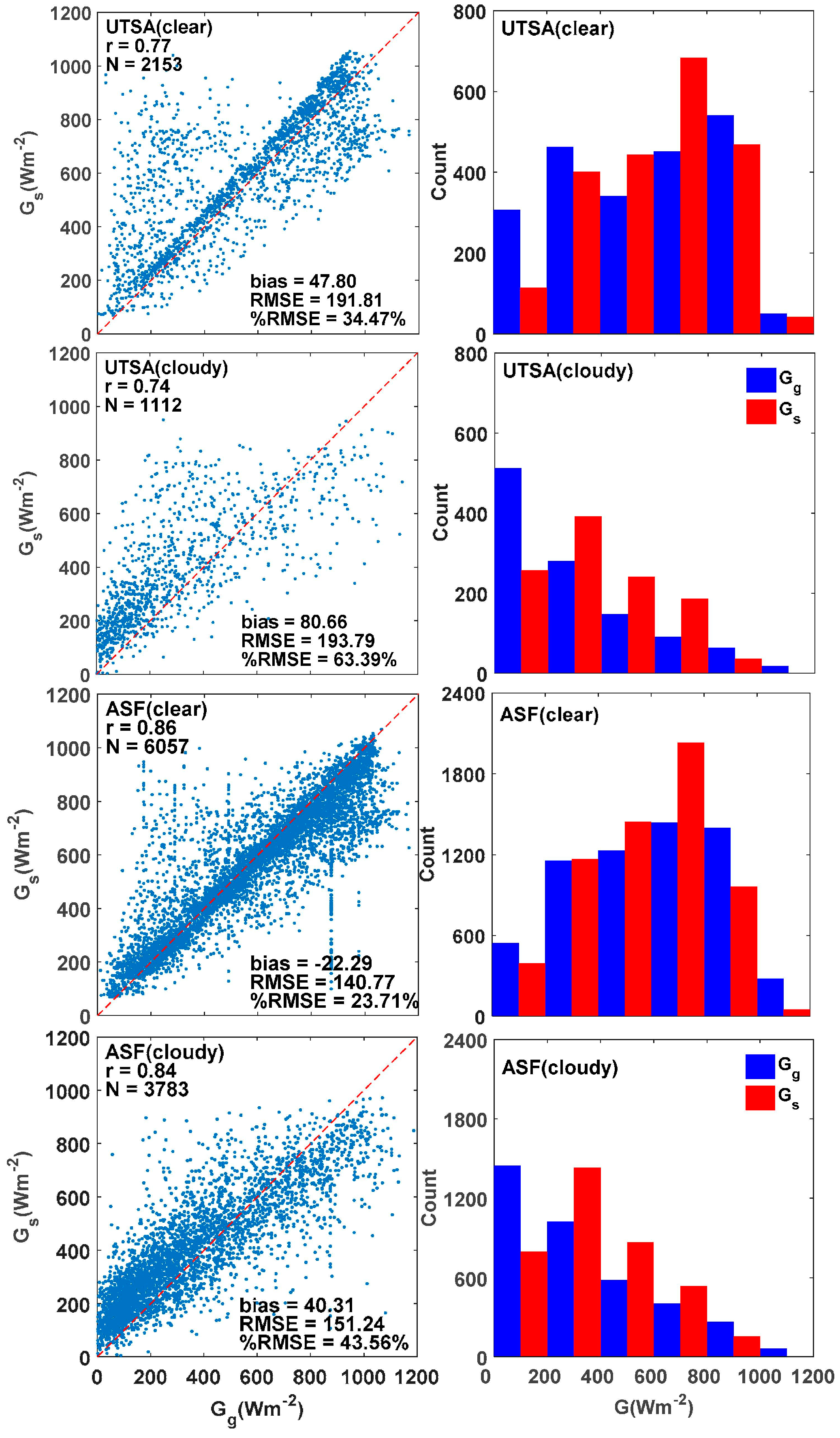
4.3. Comparison of Gs and Gg on an Hourly Timescale under Clear-Sky and Cloudy-Sky Conditions

On an hourly basis, Gs and Gg are compared separately for clear-sky and cloudy-sky conditions in Figure 4. It is interesting to see that, by separating clear-sky from cloudy-sky conditions, the correlation coefficients between Gs and Gg slightly decrease to, respectively, 0.77 and 0.86 for clear-sky condition and 0.74 and 0.84 for cloudy-sky conditions on an hourly timescale at UTSA and ASF. As expected, the comparisons show higher scatter for cloudy-sky conditions than for clear-sky conditions at both sites. As noted before, Gs appears to lie above the 1:1 line when G is low and lie below the line when G is high, which indicates that Gs often overestimates when G is low and underestimates when G is high. As can be seen from the histograms, solar irradiance under clear-sky conditions falls in the whole range of 0–1200 Wm−2 with peaks falling between 800 to 1000 Wm−2, while under cloudy-sky condition it mainly falls in the lower ranges, which indicate that clouds attenuate solar radiation reaching the surface of the Earth. Therefore, the frequency counts of Gs and Gg for cloudy-sky conditions are higher in the lower range of solar irradiance than in the higher range. Also, the biases at the ASF site are smaller than those at the UTSA site. They are negative under clear-sky conditions and positive under cloudy-conditions at the ASF site.

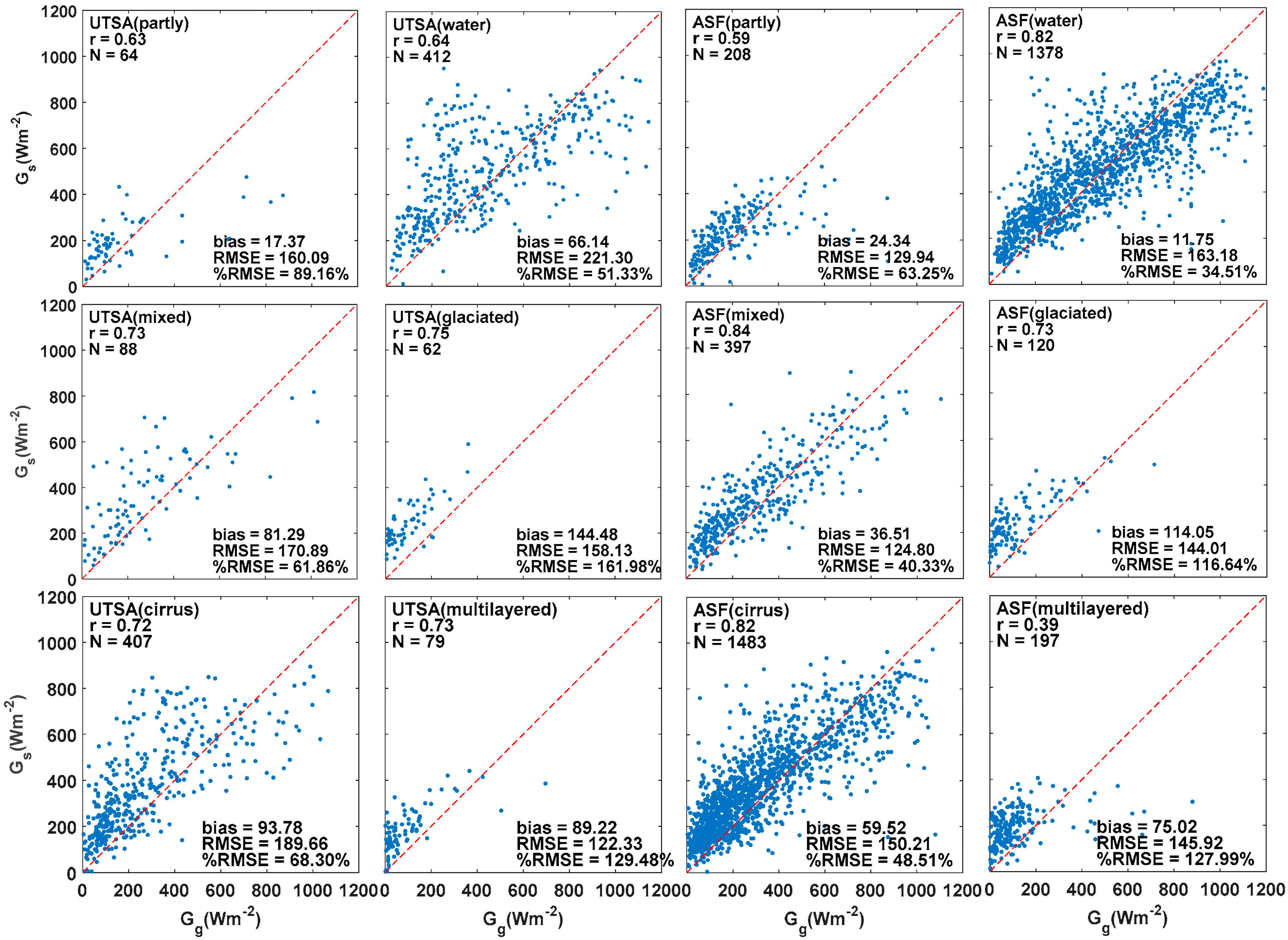
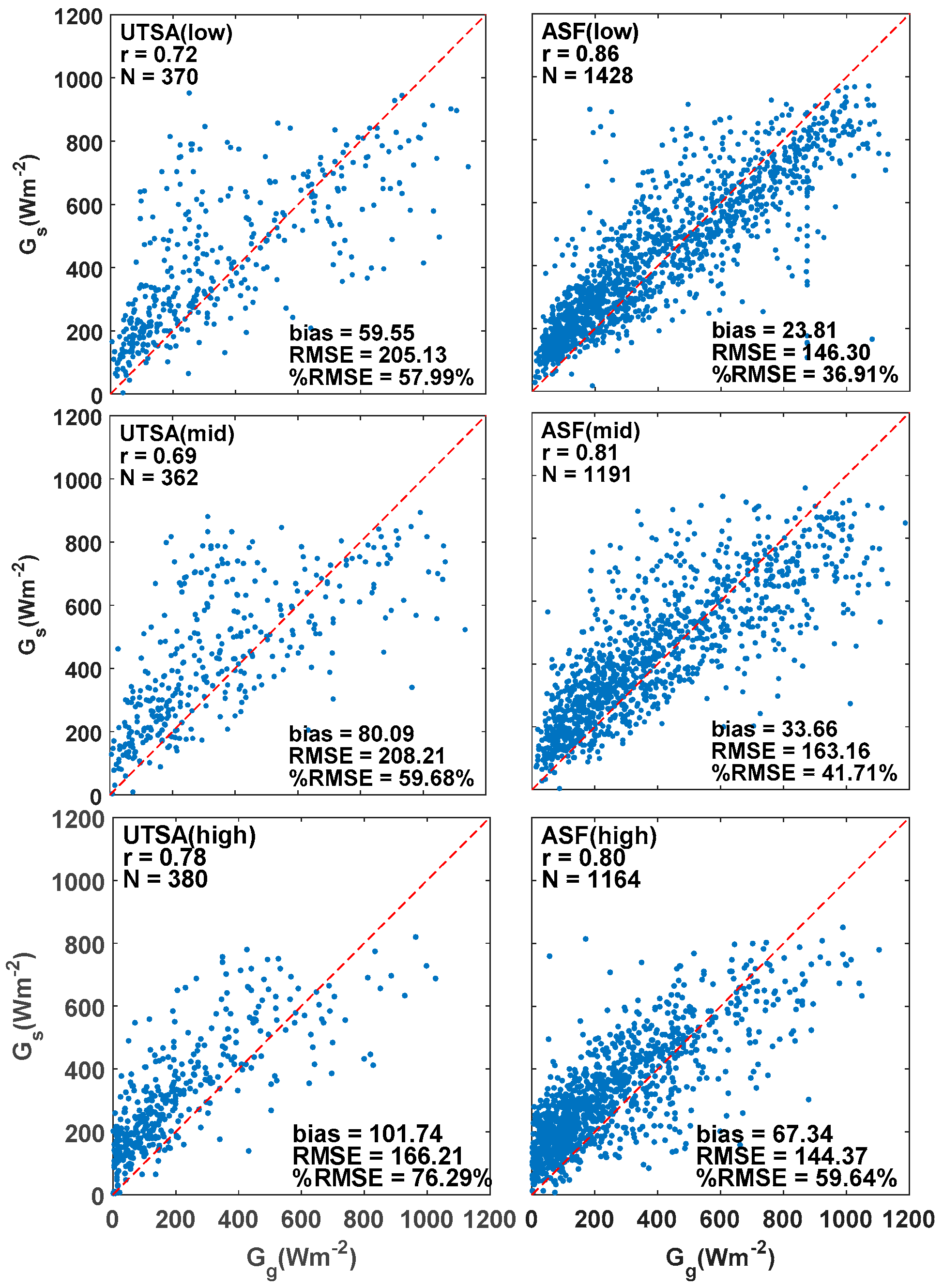
4.4. Comparison of Gs and Gg on an Hourly Timescale under Different Cloud Types and Layers

Figure 5 shows that the correlations between Gs and Gg under different cloud types are ~0.6 or greater except for the multilayered cloud type at the ASF site. The absolute values of the bias is smallest for the partly cloudy type at the UTSA site and the water cloud type at the ASF site, and highest for glaciated clouds at both sites. RMSE is highest for water cloud type at both sites and lowest for the multilayered cloud type at the UTSA site and the mixed cloud type at ASF site.
Figure 6 shows that the correlation coefficients between Gs and Gg at low, mid and high cloud layers, are all higher than 0.60 with the bias absolute values being lowest for the low cloud layer and highest for the high cloud layer. RMSEs are lowest for the high cloud layer and highest for the mid cloud layer. As always, the absolute value of biases and RMSEs are mostly smaller at the ASF site than those at the UTSA site, while the opposite is true for the correlation coefficients.

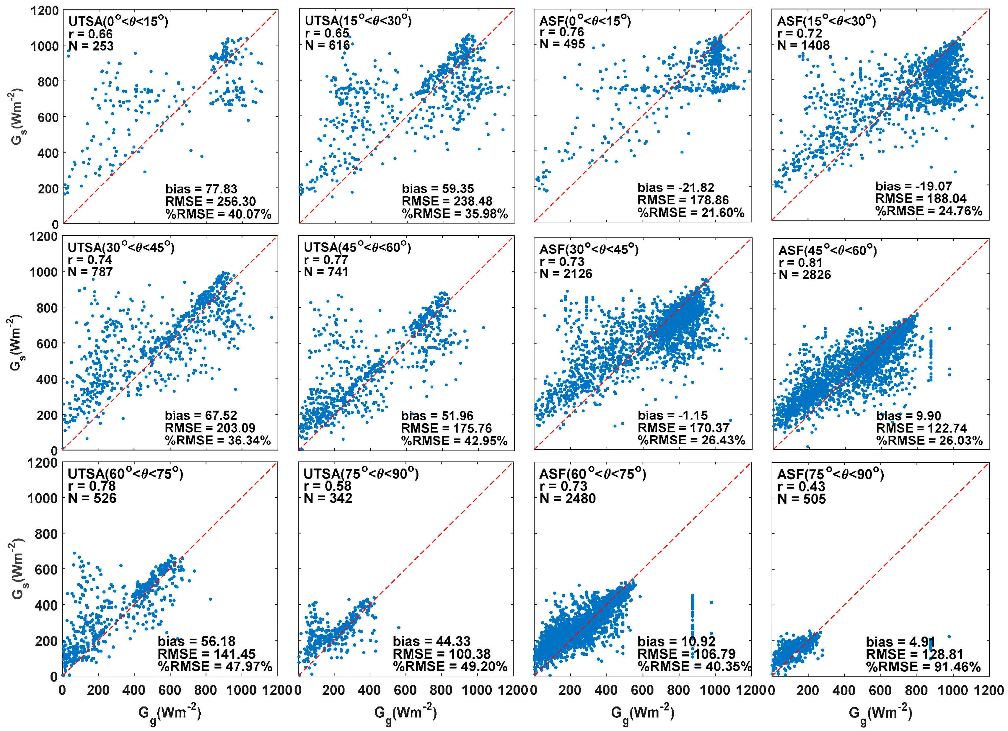
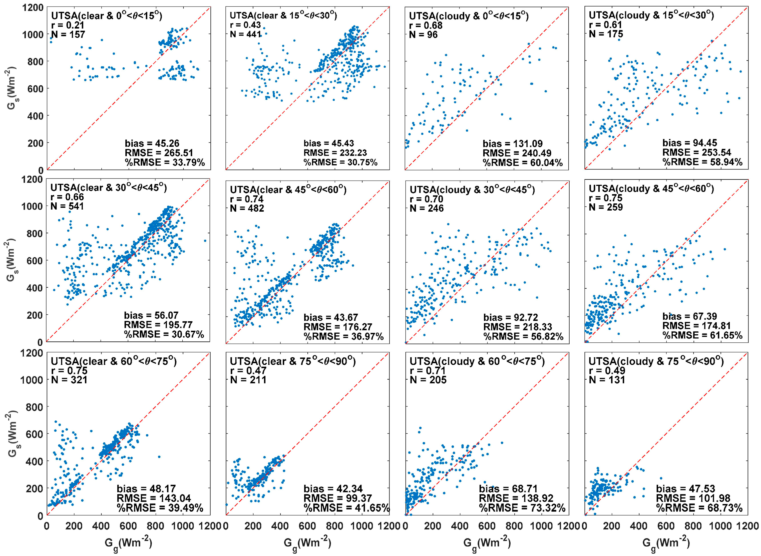
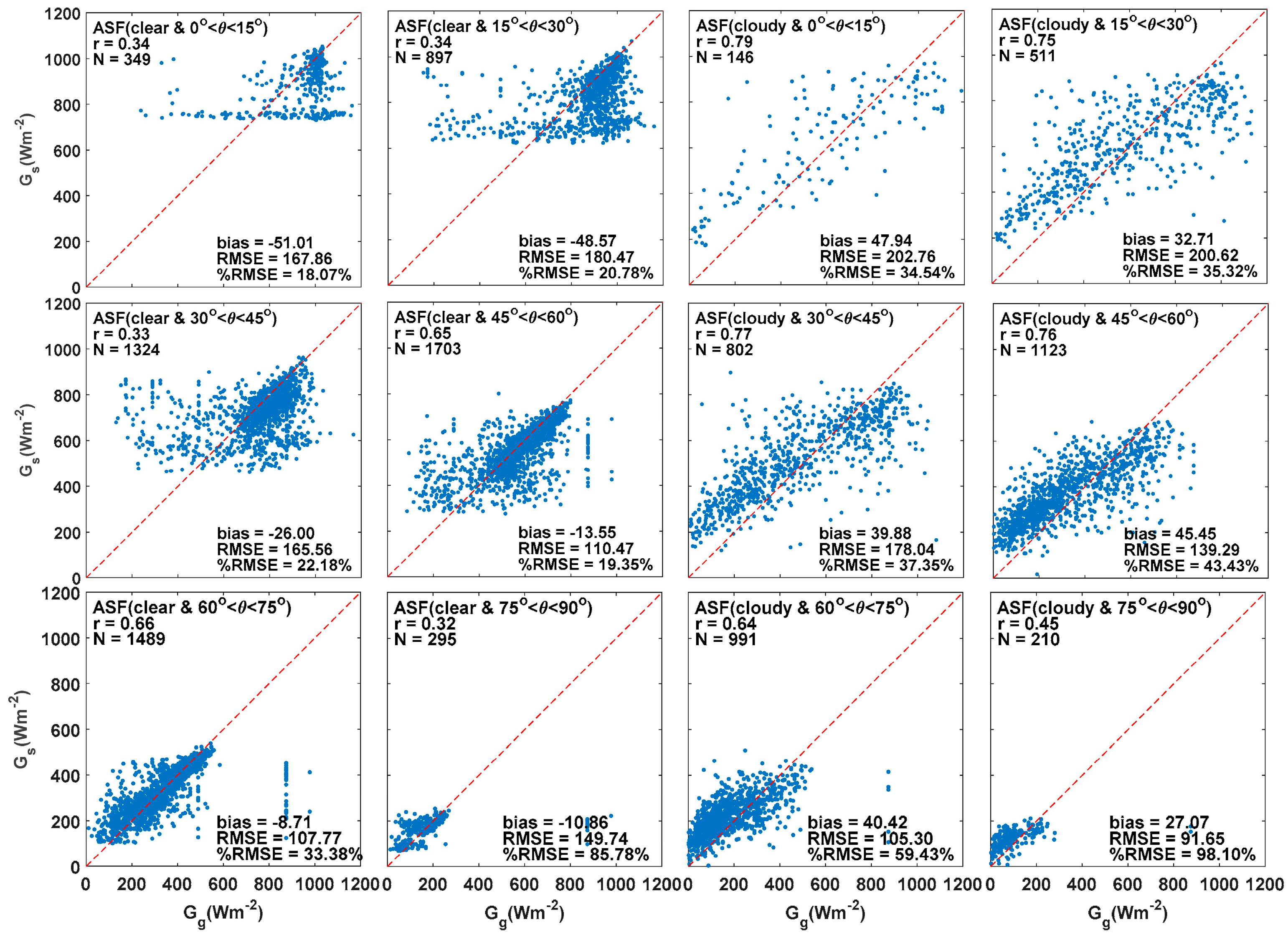
4.5. Comparison of Gs and Gg on an Hourly Timescale Under Different Solar Zenith Angles

Based on the availability of Gs in the GSIP product and Gg, the solar zenith angle ranges from 6.20° to 89.80° at the UTSA site and ranges from 6.19° to 83.52° at the ASF site. Figure 7 shows the comparison between Gs and Gg under all sky conditions on an hourly scale and for the following six intervals of the solar zenith angle: 0–15°, 15–30°, 30–45°, 45–60°, 60–75°, and 75–90°. As seen from these comparisons, the correlation coefficients are smallest with solar zenith angles in the range of 75–90° at both sites. Again, the absolute values of biases and RMSEs are mostly smaller at the ASF site as compared to the corresponding one at the UTSA site, and the biases are all positive at the UTSA site while they are negative with solar zenith angles in the range of 0–45° at the ASF site.
Figure 8 and Figure 9 show the correlations between Gs and Gg at five intervals of solar zenith angles under clear-sky and cloudy-sky conditions at the two sites. The correlation coefficients are always greater under cloud-sky conditions than the corresponding ones under clear-sky conditions, except at the solar zenith angle of 60–75° at both sites (0.75 and 0.66 under clear-sky conditions versus 0.71 and 0.64 under cloudy-sky conditions). Contrary to expectation, overall the correlation coefficients increase with the increasing solar zenith angle under clear-sky conditions except for 75–90°, which might be caused by the misspecification of aerosol optical depth and surface albedo in the GSIP algorithm and deserves further examinations [18].

5. Discussion

This study compares the Gs and Gg mainly on the hourly timescale, under clear and various cloudy-sky conditions, at different solar zenith angles, and at two different sites in San Antonio, Texas, USA. Due to the difference in spectral range and the pyranometer calibrations at the two sites (0.4–1.1 µm at the UTSA site and 0.285–2.8 µm at the ASF site), a bias could be induced in Gg. The larger errors found in the comparison at the UTSA site could be explained by the spectral range at the UTSA site pyranometer being less than that at the ASF site and the potentially improper calibration of the pyranometer at the UTSA site. The Gg at the UTSA site is always relatively smaller than that at the ASF site, although the Gs at the two sites would be overall the same (or similar) as expected since they are very close in space (~40 km). This explains the overall smaller Gg as compared with the corresponding Gs at the UTSA site (Figure 2 and Figure 3) and the overall positive bias of Gs at the UTSA site. Also, for both sites the uncertainties in the estimation of cloud properties (cover, type and layer) could also be another source of error. The rapid changes in cloud cover can be inferred from the ground measurements, especially at the finer resolution at the ASF site [40,41]. The different areas that the satellite sensor and ground pyranometer represent could also cause some error, especially for partially cloud-covered conditions.
As for the comparison between Gs and Gg at the ASF site, the Gs biases are lower (Figure 2 and Figure 3), which is similar to the previous studies under all sky conditions, with bias of 1.77 Wm−2 (ASF site) vs. −36–5 Wm−2 (previous studies) on the hourly timescale, and 2.77 Wm−2 (ASF site) vs. −11–8 Wm−2 (previous studies) on the daily timescale [12,13,14,15,16,17,18,42]. However, the RMSE at the ASF site is relatively higher than that of previous studies: 144.89 Wm−2 vs. 63–104 Wm−2 on the hourly scale and 74.00 Wm−2 vs. 15–49 Wm−2 on the daily scale.
The most novel aspect of this study as compared with previous studies is that we compare Gs and Gg under all sky and different cloudy-sky conditions and at different solar zenith angles. The correlation coefficients between Gs and Gg and the RMSE at the ASF site are similar under clear-sky and cloudy-sky conditions, although the %RMSE under the clear-sky conditions is 20% smaller than that under cloudy-sky conditions (i.e., 23.71% vs. 43.56%, Figure 4). This indicates that the satellite can map the surface solar radiance better in clear-sky conditions than in cloudy-sky conditions. The miscalculation of clear conditions as cloudy could cause the underestimates in Gs of GSIP, which resulted in negative bias [43]. Cloudy fragmentation could be another reason that contributes to a larger bias in Gs [44]. The bias under clear-sky conditions is negative, while it is positive under cloudy-sky conditions (−22.29 Wm−2 vs. 40.31 Wm−2, Figure 4). Compared with Habte et al. [17], the results in the two studies are consistent in terms of correlation coefficients, i.e., better correlation under clear-sky conditions than under cloudy-sky conditions, but they differ in terms of bias; that is, higher bias under clear-sky conditions than under cloudy-sky conditions in Habte et al. [17]. This consistent result further supports that the satellite underperforms under cloudy-sky conditions with high errors [18].
Under all sky and clear-sky conditions, the overall correlation coefficient between Gs and Gg increases and the absolute values of bias and RMSE of Gs decreases, as the solar zenith angle increases except for 75–90° (Figure 7 and Figure 9); under cloudy-sky conditions, the overall correlation coefficient between Gs and Gg and the absolute values of bias decrease as the solar zenith angle increases (Figure 9). Higher bias at the low solar zenith angle under all sky and clear-sky conditions found in this study is consistent with the reports from Habte et al. [17]. A possible explanation of this is that the GSIP model reports lower Gs under clear-sky conditions, especially around solar noon (low solar zenith angle), when the solar irradiance values are the highest [17]. The correlation coefficients are the smallest at the largest solar zenith angle interval, which could be a result of less accuracy in the retrieval of cloud properties from satellites (Figure 8) [40].

6. Conclusions

This paper examines the correlations between Gs and Gg on different timescales (mainly hourly), under different sky conditions, different cloud categories and solar zenith angles. The correlation from the two sites shows Gs is in good agreement with Gg (0.80–0.87 on the hourly timescale and 0.94–0.91 on the daily timescale) and the trends and patterns of Gs and Gg are quite similar under both clear-sky and cloudy-sky conditions, although it is clear that the magnitude of Gg measured in the UTSA site was smaller than that from the GOES satellite, potentially due to the improper calibration of the pyranometer at the UTSA site. To our knowledge, this study is the first to examine the effects of different cloud types, cloud heights, and solar zenith angles on the solar surface irradiance mapped from the GOES satellite. It is found that errors in cases of cloudy-sky conditions are higher than those under clear-sky conditions. In terms of cloud type, the correlation coefficient between Gs and Gg was the highest (r = 0.94) for the mixed cloud type at the ASF site. Overall, the correlation coefficient between Gs and Gg decreases (and the absolute values of bias and RMSE decrease) with the increase of solar zenith angle for cloudy-sky conditions. The correlation coefficients are mostly greater under cloud-sky conditions than the corresponding ones under clear-sky conditions. It is necessary to point out that the significance of this comparison between Gs and Gg is that it validates the GOES products in the San Antonio, Texas, USA area. With the above statistics, it can be seen that the real-time satellite estimates from GOES, Gs, are thus reliable and acceptable for future application on solar mapping and forecasting in this region.

Acknowledgments

This work is supported by CPS Energy and Texas Sustainable Energy Research Institute (TSERI).

Author Contributions

Rolando Vega, Hongjie Xie, Alberto M. Mestas-Nuñez contributed the main idea; Shuang Xia performed the data processing, analysis and paper writing; Hongjie Xie and Alberto M. Mestas-Nuñez contributed to the paper writing and conclusion abstraction; all authors contributed to the revision and edits.

Conflicts of Interest

The authors declare no conflict of interest.

References

  1. Bahnemann, D. Photocatalytic water treatment: Solar energy applications. Sol. Energy 2004, 77, 445–459. [Google Scholar] [CrossRef]
  2. Malato, S.; Maldonado, M.I.; Fernandez-Ibanez, P.; Oller, I.; Polo, I.; Sanchez-Moreno, R. Decontamination and disinfection of water by solar photocatalysis: The pilot plants of the Plataforma Solar de Almeria. Mater. Sci. Semicond. Process. 2016, 42, 15–23. [Google Scholar] [CrossRef]
  3. Byrne, J.A.; Fernandez-Ibanez, P.A.; Dunlop, P.S.M.; Alrousan, D.M.A.; Hamilton, J.W.J. Photocatalytic Enhancement for Solar Disinfection of Water: A Review. Int. J. Photoenergy 2011. [Google Scholar] [CrossRef]
  4. Jasrotia, S.; Kansal, A.; Kishore, V.V.N. Application of solar energy for water supply and sanitation in Arsenic affected rural areas: A study for Kaudikasa village, India. J. Clean. Prod. 2013, 60, 102–106. [Google Scholar] [CrossRef]
  5. Samimi, A.; Zarinabadi, S.; Samimi, M. Solar Energy Application on Environmental Protection. Int. J. Sci. Investig. Fr. 2012, 1, 21–24. [Google Scholar]
  6. Novacheck, J.; Johnson, J.X. The environmental and cost implications of solar energy preferences in Renewable Portfolio Standards. Energy Policy 2015, 86, 250–261. [Google Scholar] [CrossRef]
  7. Hernandez, R.R.; Easter, S.B.; Murphy-Mariscal, M.L.; Maestre, F.T.; Tavassoli, M.; Allen, E.B.; Barrows, C.W.; Belnap, J.; Ochoa-Hueso, R.; Ravi, S.; et al. Environmental impacts of utility-scale solar energy. Renew. Sustain. Energy Rev. 2014, 29, 766–779. [Google Scholar] [CrossRef]
  8. Hosseini, S.E.; Andwari, A.M.; Wahid, M.A.; Bagheri, G. A review on green energy potentials in Iran. Renew. Sustain. Energy Rev. 2013, 27, 533–545. [Google Scholar] [CrossRef]
  9. Abas, N.; Kalair, A.; Khan, N. Review of fossil fuels and future energy technologies. Futures 2015, 69, 31–49. [Google Scholar] [CrossRef]
  10. Pinker, R.T.; Laszlo, I.; Tarpley, J.D.; Mitchell, K. Geostationary satellite parameters for surface energy balance. Adv. Space Res. 2002, 30, 2427–2432. [Google Scholar] [CrossRef]
  11. Laszlo, I.; Ciren, P.; Liu, H.; Kondragunta, S.; Tarpley, J.D.; Goldberg, M.D. Remote sensing of aerosol and radiation from geostationary satellites. Adv. Space Res. 2008, 41, 1882–1893. [Google Scholar] [CrossRef]
  12. Pinker, R.T.; Ewing, J. Modeling surface solar radiation: Model formulation and validation. J. Clim. Appl. Meteorol. 1985, 24, 389–401. [Google Scholar] [CrossRef]
  13. Pinker, R.T.; Tarpley, J.D.; Laszlo, I.; Mitchell, K.E.; Houser, P.R.; Wood, E.F.; Schaake, J.C.; Robock, A.; Lohmann, D.; Cosgrove, B.A.; et al. Surface radiation budgets in support of the GEWEX Continental-Scale International Project (GCIP) and the GEWEX Americas Prediction Project (GAPP), including the North American Land Data Assimilation System (NLDAS) project: GEWEX Continental-Scale International Project, Part 3 (GCIP3). J. Geophys. Res. 2003, 108. [Google Scholar] [CrossRef]
  14. Augustine, J.A.; DeLuisi, J.J.; Long, C.N. SURFRAD—A national surface radiation budget network for atmospheric research. Bull. Am. Meteorol. Soc. 2000, 81, 2341–2357. [Google Scholar] [CrossRef]
  15. Meng, C.J.; Pinker, R.T.; Tarpley, J.D.; Laszlo, I. A satellite approach for estimating regional land surface energy budget for GCIP/GAPP. J. Geophys. Res. 2003, 108. [Google Scholar] [CrossRef]
  16. Otkin, J.A.; Anderson, M.C.; Mecikalski, J.R.; Diak, G.R. Validation of GOES-based insolation estimates using data from the US Climate Reference Network. J. Hydrometeorol. 2005, 6, 460–475. [Google Scholar] [CrossRef]
  17. Habte, A.; Sengupta, M.; Wilcox, S. Comparing Measured and Satellite-Derived Surface Irradiance. In Proceedings of the ASME 2012 6th International Conference on Energy Sustainability collocated with the ASME 2012 10th International Conference on Fuel Cell Science, Engineering and Technology, San Diego, CA, USA, 23–26 July 2012; pp. 561–566. [Google Scholar]
  18. Habte, A.; Sengupta, M.; Wilcox, S. Validation of GOES-Derived Surface Radiation Using NOAA’s Physical Retrieval Method; Technical Report NREL/TP-5500-57442; National Renewable Energy Laboratory: Golden, CO, USA, 2013. [CrossRef]
  19. Zidanšek, A.; Ambrožič, M.; Milfelner, M.; Blinc, R.; Lior, N. Solar orbital power: Sustainability analysis. Energy 2011, 36, 1986–1995. [Google Scholar] [CrossRef]
  20. Escrig, H.; Batlles, F.J.; Alonso, J.; Baena, F.M.; Bosch, J.L.; Salbidegoitia, I.B.; Burgaleta, J.I. Cloud detection, classification and motion estimation using geostationary satellite imagery for cloud cover forecast. Energy 2013, 55, 853–859. [Google Scholar] [CrossRef]
  21. Kleissl, J. Solar Energy Forecasting and Resource Assessment; Academic Press: Cambridge, MA, USA, 2013; pp. 50–76. [Google Scholar]
  22. Pinker, R.T.; Laszlo, I. Modeling surface solar irradiance for satellite applications on a global scale. J. Appl. Meteorol. 1992, 31, 194–211. [Google Scholar] [CrossRef]
  23. Pinker, R.T.; Laszlo, I. Global distribution of photosynthetically active radiation as observed from satellites. J. Clim. 1992, 5, 56–65. [Google Scholar] [CrossRef]
  24. Mesinger, F.; Black, T.L. On the impact on forecast accuracy of the step-mountain (eta) vs. sigma coordinate. Meteorol. Atmos. Phys. 1992, 50, 47–60. [Google Scholar] [CrossRef]
  25. Black, T.L. The new NMC mesoscale Eta model: Description and forecast examples. Weather Forecast. 1994, 9, 265–278. [Google Scholar] [CrossRef]
  26. Tarpley, J.D.; Pinker, R.T.; Laszlo, I. Experimental GOES shortwave radiation budget for GCIP. In Proceedings of the Second International Scientific Conference on the Global Energy and Water Cycle, Washington, DC, USA, 17–21 June 1996; pp. 17–21. [Google Scholar]
  27. Rogers, E.; Black, T.L.; Deaven, D.G.; DiMego, G.J.; Zhao, Q.; Baldwin, M.; Junker, N.W.; Lin, Y. Changes to the operational “early” Eta analysis/forecast system at the National Centers for Environmental Prediction. Weather Forecast. 1996, 11, 391–413. [Google Scholar] [CrossRef]
  28. Stephens, G.L.; Ackerman, S.; Smith, E.A. A shortwave parameterization revised to improve cloud absorption. J. Atmos. Sci. 1984, 41, 687–690. [Google Scholar] [CrossRef]
  29. Lave, M.; Kleissl, J. Optimum fixed orientations and benefits of tracking for capturing solar radiation in the continental United States. Renew. Energy 2011, 36, 1145–1152. [Google Scholar] [CrossRef]
  30. Pavolonis, M.J.; Heidinger, A.K.; Uttal, T. Daytime global cloud typing from AVHRR and VIIRS: Algorithm description, validation, and comparisons. J. Appl. Meteorol. 2005, 44, 804–826. [Google Scholar] [CrossRef]
  31. Reno, M.J.; Stein, J.S. Using cloud classification to model solar variability. In Proceedings of the ASES National Solar Conference, Baltimore, MD, USA, 16–20 April 2013. [Google Scholar]
  32. Vignola, F.; Michalsky, J.; Stoffel, T. Solar and Infrared Radiation Measurements; CRC Press: Boca Raton, FL, USA, 2016. [Google Scholar]
  33. Mellit, A.; Pavan, A.M. A 24-h forecast of solar irradiance using artificial neural network: Application for performance prediction of a grid-connected PV plant at Trieste, Italy. Sol. Energy 2010, 84, 807–821. [Google Scholar] [CrossRef]
  34. Stephens, G.L. Radiation profiles in extended water clouds. I: Theory. J. Atmos. Sci. 1978, 35, 2111–2122. [Google Scholar] [CrossRef]
  35. Jang, J.; Lee, C.; Hahn, J.W. Theoretical study on evaporation of sessile water droplets on a glass panel with infrared radiation. J. Mech. Sci. Technol. 2014, 28, 1575–1580. [Google Scholar] [CrossRef]
  36. Fan, J.W.; Leung, L.R.; Rosenfeld, D.; DeMott, P.J. Effects of cloud condensation nuclei and ice nucleating particles on precipitation processes and supercooled liquid in mixed-phase orographic clouds. Atmos. Chem. Phys. 2017, 17, 1017–1035. [Google Scholar] [CrossRef]
  37. Cintineo, J.L.; Pavolonis, M.J.; Sieglaff, J.M.; Heidinger, A.K. Evolution of Severe and Nonsevere Convection Inferred from GOES-Derived Cloud Properties. J. Appl. Meteorol. Climatol. 2013, 52, 2009–2023. [Google Scholar] [CrossRef]
  38. Kayetha, V.K. Ice Clouds over Fairbanks, Alaska. Master’s Thesis, University of Alaska Fairbanks, Fairbanks, AK, USA, 2014. [Google Scholar]
  39. Martin, J. Wild Weather (Oxford Read and Discover Level 5); Oxford University Press: Oxford, UK, 2015. [Google Scholar]
  40. Qu, Z.; Oumbe, A.; Blanc, P.; Espinar, B.; Gesell, G.; Gschwind, B.; Klüser, L.; Lefèvre, M.; Saboret, L.; Schroedter-Homscheidt, M.; et al. Fast radiative transfer parameterisation for assessing the surface solar irradiance: The Heliosat-4 method. Meteorologische Zeitschrift 2017, 26, 33–57. [Google Scholar] [CrossRef]
  41. Bengulescu, M.; Blanc, P.; Boilley, A.; Wald, L. Do modelled or satellite-based estimates of surface solar irradiance accurately describe its temporal variability? Adv. Sci. Res. 2017, 14, 35–48. [Google Scholar] [CrossRef]
  42. Masuda, K. Surface radiation budget: Comparison between global satellite-derived products and land-based observations in Asia and Oceania. In Proceedings of the International Radiation Symposium, Busan, Korea, 23–28 August 2014. [Google Scholar]
  43. Eissa, Y.; Korany, M.; Aoun, Y.; Boraiy, M.; Abdel Wahab, M.M.; Alfaro, S.C.; Blanc, P.; EI_Metwally, M.; Ghedira, H.; Hungershoeder, K.; et al. Validation of the surface downwelling solar irradiance estimates of the HelioClim-3 database in Egypt. Remote Sens. 2015, 7, 9269–9291. [Google Scholar] [CrossRef] [Green Version]
  44. Marie-Joseph, I.; Linguet, L.; Gobinddass, M.L.; Wald, L. On the applicability of the Heliosat-2 method to assess surface solar irradiance in the Intertropical Convergence Zone, French Guiana. Int. J. Remote Sens. 2013, 34, 3012–3027. [Google Scholar] [CrossRef] [Green Version]
Figure 1. Map of the state of Texas showing the locations of the City of San Antonio (left panel) and of the in situ measurement sites, UTSA and ASF, relative to main roads in the San Antonio Area (right panel).
Remotesensing 09 01268 g001
Figure 2. Mean hourly surface solar irradiance Gs (red solid) and Gg (blue dash) and total number of pairs (black dash) plotted against the time of day (hours) for clear-sky and cloudy-sky conditions, during the respective time periods: 1 May–25 October 2015 at the UTSA site (left two panels) and July–September 2014 and 22 September 2015–18 October 2016 at the ASF site (right two panels).
Remotesensing 09 01268 g002
Figure 3. Scatter plots showing the correlation of Gs versus Gg on hourly and daily timescales for all-sky conditions at UTSA (left panel) and ASF (right panel) with the corresponding statistical parameters, r, bias, RMSE, %RMSE and N (number of observation pairs). The units of bias and RMSE are in Wm−2. The red-dash lines indicate the one-to-one lines.
Remotesensing 09 01268 g003
Figure 4. Scatter plots showing the correlation of hourly Gs versus Gg for clear-sky and cloudy-sky conditions at UTSA (upper two panels) and ASF (bottom two panels). The corresponding histograms of Gs versus Gg are shown in the right panel with the red indicating Gs and the blue indicating Gg.
Remotesensing 09 01268 g004
Figure 5. Scatter plots showing the correlation of Gs versus Gg for the six different cloud types at UTSA (left two panels) and ASF (right two panels).
Remotesensing 09 01268 g005
Figure 6. Scatter plots showing the correlation of Gs versus Gg for the three cloud layers (low, mid, and high) at UTSA (left panel) and ASF (right panel).
Remotesensing 09 01268 g006
Figure 7. Scatter plots showing the comparisons of Gs with Gg for various intervals of solar zenith angle at UTSA (left two panels) and ASF (right two panels).
Remotesensing 09 01268 g007
Figure 8. Scatter plots showing the comparisons of Gs with Gg for various intervals of solar zenith angle for clear-sky (left two panels) and cloudy-sky (right two panels) conditions, respectively at the UTSA site.
Remotesensing 09 01268 g008
Figure 9. Same as Figure 8 but for the ASF site.
Remotesensing 09 01268 g009
Table 1. GOES surface and insolation products cloud categories adapted from [31].
Cloud CategoryClassified IDDescription
Cloud type0Clear
1partly (partly cloudy/fog)
2water(water cloud)
3mixed (supercooled/mixed-phase cloud)
4glaciated (optically thick ice cloud)
5cirrus (optically thin ice cloud)
6multi-layered(cirrus over lower cloud)
Cloud layer1low (0–2 km)
2mid (2–7 km)
3high (5–13 km)
Table 2. The number and percentages of occurrence of clear-sky and cloudy-sky conditions from GOES products at UTSA (1 May–25 October 2015) and ASF (July–September 2014 and 22 September 2015–18 October 2016) sites.
Clear/CloudyUTSAASF
NPercentage (%)NPercentage (%)
clear (0)215365.94605761.50
lowpartly (1)371.131211.23
water (2)2427.419419.56
mixed (3)190.19
cirrus (5)912.693483.54
midpartly (1)200.61670.68
water (2)1675.114354.42
mixed (3)561.722232.26
cirrus (5)1193.654664.74
highpartly (1)70.22200.20
water (2)30.0920.02
mixed (3)3240.981561.59
glaciated (4)621.901201.22
cirrus (5)1976.036696.80
multilayered (6)792.421972.00

