Abstract
Many soil remote sensing applications rely on narrow-band observations to exploit molecular absorption features. However, broadband sensors are invaluable for soil surveying, agriculture, land management and mineral exploration, amongst others. These sensors provide denser time series compared to high-resolution airborne imaging spectrometers and hold the potential of increasing the observable bare-soil area at the cost of spectral detail. The wealth of data coming along with these applications can be handled using cloud-based processing platforms such as Earth Engine. We present a method for identifying the least-vegetated observation, or so called barest pixel, in a dense time series between January 1985 and March 2017, based on Landsat 5, 7 and 8 observations. We derived a Barest Pixel Composite and Bare Soil Composite for the agricultural area of the Swiss Plateau. We analysed the available data over time and concluded that about five years of Landsat data were needed for a full-coverage composite (90% of the maximum bare soil area). Using the Swiss harmonised soil data, we derived soil properties (sand, silt, clay, and soil organic matter percentages) and discuss the contribution of these soil property maps to existing conventional and digital soil maps. Both products demonstrate the substantial potential of Landsat time series for digital soil mapping, as well as for land management applications and policy making.
1. Introduction
Soils are often at the heart of the services that ecosystems deliver, not only in terms of food production, but also in filtering, the cycling of nutrients, the storage and regulation of water and providing habitats for soil biota [1]. However, soils are under increasing pressure as a result of overuse [2], leading to an alteration and reduction of its provided services. Soil services may further degrade due to erosion, dust storms, salinisation, pollution, compaction, depletion, decomposition of organic matter and the destruction of soil aggregates [2]. At the same time, an expansion and intensification of the agricultural area is necessary in order to meet the expected demand for food [3] because of the growth of the population and wealth. Since degraded soil is not renewed easily and in order to secure soil functions in the future [4], the mapping of soil properties and functions and the monitoring of changes over time are important. Especially, spatially distributed soil information has become more important with the use of global and regional models, which often require full coverage soil information [5]. The use of remote sensing can offer spatial temporal, and quantitative soil information of extended areas [6], which can be acquired with limited fieldwork.
Soil remote sensing today can explore narrow spectral absorption features using imaging spectroscopy data. This has found applications in soil surveying, agriculture, land management and mineral exploration (for extensive reviews, we refer to [5,6,7,8]). Today, however, multispectral sensors provide invaluable time series of data since the 1970s with global coverage. Several studies have shown that multispectral data can be used for soil applications despite spectral features of soils often being weak, narrow and mixed [6]. For instance, Demattê et al. [9] predicted different physical and chemical soil attributes in an area in Brazil using a single Landsat ETM+ 7 (Landsat 7 Enhanced Thematic Mapper+) image and showed promising results for clay and sand. Nanni et al. [10] used similar methods to discriminate soil pixels into the different soil classes in a study area in Brazil. This showed that 14 out of 16 soil classes could be predicted with a success rate of >40%. Similar studies with satellite sensors were conducted by Shabou et al. [11] and Fioirio et al. [12].
However, around 56% of the global land areas are covered by green vegetation [13]. Therefore, in these studies, the application is limited to the amount of bare soil visible in a single acquisition. This reduces the usability of remote sensing techniques in soil science, especially for generating large and continuous soil maps showing the spatial variation of different soil properties. To reduce this problem, several studies used multi-temporal images [14,15,16]. In areas with agriculture, crop rotation or other alternation between bare and vegetated states, such multi-temporal images can be used to increase the amount of observed bare soil [16]. Demattê et al. [15] analysed five satellite images from five consecutive years over the same area and captured in the same season. With this method, they could increase the total bare soil area from 36% in a single image to 85% for the fused image. Diek et al. [16] applied a similar approach with airborne imaging spectroscopy data. They combined three airborne images from the same area at different dates and more than doubled the amount of bare soil pixels compared to one acquisition. These studies show that the use of multi-temporal remote sensing can be used to increase the amount of spectral bare soil information. However, the methods were limited to a handful of scenes.
We now used all available Landsat scenes between 1985 and 2017 in order to maximize the bare soil coverage over a large agricultural area. We built on the methodology for creating the well-established Greenest Pixel Composite and aimed to modify this to detect the least-vegetated observation in a dense time series of Landsat resulting in the counterpart, the Barest Pixel Composite. The large amounts of data that attend these Landsat time series can be handled using recent developments in image analysis, including the Google Earth Engine (GEE) platform [17]. The value of the GEE platform for digital soil mapping has already been demonstrated using soil profile data and various topographical and meteorological covariates [18]. We explored the availability of the satellite data and the Swiss harmonised soil data over time in order to define the aggregation window (in years) that is needed for a full-coverage soil product. Based on a bare soil index, we created the Barest Pixel Composite for the agricultural area of the Swiss Plateau. We used imaging spectroscopy data to define a spectral threshold for bare soil detection in Landsat data and generated the according Bare Soil Composite that we used for predicting soil properties (sand, silt, clay and soil organic matter). Finally, we show a comparison between the remote sensing soil property maps and available conventional and digital soil maps.
2. Study Area
Switzerland can be divided in three geographical regions: (I) the Jura, (II) The Swiss Plateau and (III) the Alps. The Swiss Plateau covers ca. 30% of Switzerland and cover an area of 1,249,875.5 ha (Figure 1). At the same time, two-thirds of the population and the majority of industry, manufacturing and farming are located in the Swiss Plateau. It is bordered by Lake Geneva in the southwest, Lake Constance and the Rhine in the northeast, the Jura in the north and the foot of the Alps in the south. The average elevation is ca. 580 m, the highest point is located in the southeast (1304 m) and the lowest point is in the Rhine valley close to Basel (244 m). The climate is classified as a Maritime Temperate climate. Temperatures range between −1 and 1 °C in January and between 16 and 20 °C in July, and they decrease from west to east. Annual precipitation ranges from 800 mm near the Jura to ca. 1400 mm at the foothills of the Alps. Snow is rare, but present depending on the height. In winter, the valleys experience fog. The main categories of land use are agriculture (49.5%); forests and woodland (24.3%); and built-up (16%) [19]. The agricultural area is covered by permanent grassland (60%), arable land (39%) and special crops (1%), e.g., orchards, vineyards, or vegetables. Farms are generally small and the main crop types are (silage) maize, winter wheat, triticale, and winter barley [20]; temporary grassland is commonly included in the crop rotation.
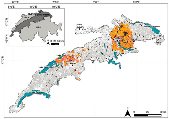
Figure 1.
Study area: The Swiss Plateau. Upper left: the Swiss Plateau (dark grey) is located in Switzerland between the Jura and the Alps (light grey). The Swiss Plateau is characterised by its agricultural area in grey and the lakes in blue. Several main cities, lakes and peaks are indicated with their name, as well as the lowest and highest point. In black small dots all soil measurements of the national soil database of Switzerland (NABODAT) dataset, in orange dots the soil field measurements and in red the soil laboratory measurements intersecting with the agricultural area of the Swiss Plateau.
The base geological layer of the Swiss Plateau is formed by crystalline basement. Mesozoic sediments cover this, originating from a shallow sea. On top of these sediments, you can find the Molasse formed during the Alpine origin, consisting of accumulated materials from the Alps. At the foot of the Alps, huge fans can be found (e.g., Napf and Hörnli (peak of the fan)). Conglomerates and sandstone were predominantly deposited near the Alps; in the centre, you can find mainly finer sandstones and near the Jura clays and marl. The uppermost layer was formed by the ice age glaciers. The glaciers have resulted in a hilly landscape, with many valleys, rivers and lakes. Typical glacial landforms can be found all over the Swiss Plateau [21].
The Swiss Plateau is mainly covered by Cambisols ((saure) Braunerde), which are characterised by a clear soil formation (A, B and C horizon). The valleys are characterised by Planosols (Pseudogleyige Braunerde), with dense, impermeable layers, because glaciers covered them. In the low areas around the glacial lakes, soils can be found that, without drainage, would be saturated with groundwater and pendular water (Gleyic Cambisols (Braunerde-Gley), Gleysols (Buntgley and Fahlgley), and Histosols or Histic Cambisols (Halbmoor)). Redox processes result in gleyic colour patterns and the soils contain high amounts of organic matter. A good example is the Grand Marais between Lake Neuchâtel, Lake Biel and Lake Morat. At rock outcrops, there are shallow and poorly developed soils (Regosols). Around the big rivers, Luvisols (Parabraunerde) can be found, characterised by clay leached and a clay accumulation layer. At the foot of the Alps, the soils are described as acid Cambisols (Braunpodzol and Podzolige, saure Braunerde) [22].
3. Materials and Methods
The generation of the barest pixel composite and the bare soil composite is described in the flowchart in Figure 2 and in this section we follow the same order. We describe (A) the pre-processing steps of the satellite data including the selection of the aggregation window (Section 3.1); (B) the generation of the Barest Pixel Composite, including a description of the used bare soil index (Section 3.2); and (C) the generation of the Bare Soil Composite, including the selection of the threshold (Section 3.3). Finally, we describe the methodology used for the soil property prediction based on the Bare Soil Composite, including a description of the used soil data (Section 3.4).
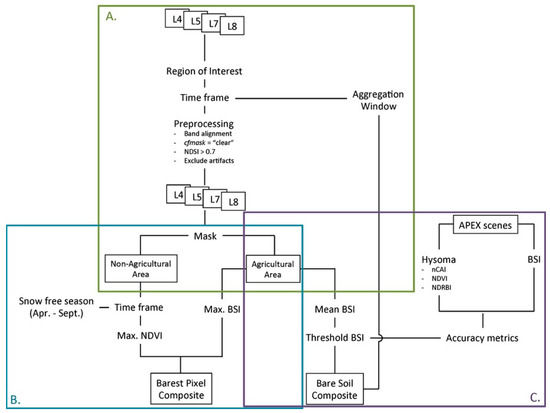
Figure 2.
Flowchart methodology: (A) preprocessing of the data (Section 3.1), (B) barest pixel composite (Section 3.2), and (C) bare soil composite (Section 3.3). Abbreviations used: L4–8 for corresponding Landsat satellites, BSI for Bare Soil Index. For other abbreviations, see Section 3.3.1.
3.1. Preprocessing
3.1.1. Satellite Data
All available Landsat surface reflectance (SR) images were collected for the period between 1 January 1985 and 1 March 2017 (n = 3030). This includes 52 Landsat scenes from Landsat 4 Thematic Mapper (L4), 731 scenes from Landsat 5 Thematic Mapper (L5), 1739 scenes from Landsat 7 Enhanced Thematic Mapper+ (L7) and 508 scenes from Landsat 8 Operational Land Imager (L8). L4 was operational between July 1982 and December 1993, L5 was operational between March 1984 and January 2013, L7 from April 1999 till present and L8 was launched in February 2013 [23]. Since 31 May 2003 the scan line corrector (SLC) of L7 failed. Without an operating SLC, the sensor records a zigzag pattern along the satellite ground track, resulting in a duplicated area. The duplicated area is removed in Level-1 processing. The remaining 78% of the pixels can be normally used [24]. For all sensors, the approximate scene size is 170 km north-south by 183 km east-west and the bands have a spatial resolution of 30 m [25]. The accuracy of the geometry is less than 12 m for all Level 1 data [26]. This means that there is a maximum inaccuracy of one pixel between two scenes.
Figure 3 shows the calculated bare soil index (BSI, Section 3.2.1) for a representative pixel in the Grand Marais area. Each point represents a satellite observation and the colours indicate the specific sensor (red: L4, purple: L5, green: L7, and orange: L8). The figure shows that very few Landsat data are available for the study area between 1990 and 2000. This was probably caused by the commercialisation strategy of NASA in the 1990s that affected the collection priorities. Furthermore, the on-board recorders of L5 broke and data could be only collected when the satellite was overhead and all the other data ended up on remote stations. We therefore excluded this time period from the analysis, including the very few available scenes. Furthermore, L4 offers very limited data in the period 1985–1990 (only 18 scenes for the full study area). We decided to exclude L4 from the analysis, since the added value for detecting bare soil is low.
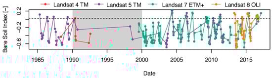
Figure 3.
Bare Soil Index (BSI) values [-] for a pixel in the bare soil area of the agricultural area of the Swiss Plateau (located in the Grand Marais). In purple L5, in green L7 and in orange L8, the dotted line is the used threshold of 0.021, in grey, the period we excluded from the analysis because Landsat data were generally not available.
We focused on the bands in the visible (VIS), near- (NIR) and shortwave- (SWIR) infrared (or VNIR–SWIR) spectral ranges (Table 1), although some Landsat sensors provide additional bands. These spectral ranges are known to contain information on soil properties [15]. Cloud-free pixels were selected based on the cfmask property (classifies every pixel according to five classes: clear, water, cloud shadow, clouds, and snow), equal to clear; snow pixels were excluded based on the normalised difference snow index (NDSI) [27], threshold of 0.7. Pixels with negative reflectance values were also excluded, as well as the upper 5% quartile of each band—both in order to remove outliers and to minimise the effects of artefacts like shades of clouds and trees, saturated pixels and coloured striping.

Table 1.
Overview of the wavelengths of the used Landsat satellite bands and their alignment.
3.1.2. Selection of Aggregation Window
The aggregation window, defined as the period needed to reach 90% of the maximum bare soil area, was calculated based on the monthly cumulative growth of the bare soil area. For five starting points (1985, 2000, 2005, 2010 and 2015), we calculated the monthly increase for time periods up to 10 years. Because of the crop rotation practices in the area, we expected a steep increase of detected bare soil area in the beginning of the time period and a slow saturation towards the maximum bare soil area. In order to explore after how much time this maximum is reached, we fitted exponential models on the monthly cumulative area for each time period. Based on these models, we estimated the total bare soil area (ha) and the time (years) required for mapping this total bare soil area. Since the fitted models are exponential and the maximum will never be reached, we considered the maximum bare soil area at 90% of the estimated total bare soil area.
3.2. Barest Pixel Composite
3.2.1. Bare Soil Index
In order to select the barest pixel in the Landsat time series, we used a bare soil index. Piyoosh and Gosh [28] give a good overview of the available bare soil indices. Many of them are not specifically developed to detect bare soil pixels, but to map bare soil and built-up area, in order to distinguish these classes or to map vegetation. Nevertheless, these are also useful to detect bare soil pixels, since reflectance response is very similar for built-up and bare soil and because low vegetation indices indicate water, snow, bare soil and built-up areas.
Given the aim to apply the bare soil index to all Landsat SR images, we only considered generic indices. Most of the indices use the thermal infrared (TIR) band or are more complex than a simple band ratio. Processing of these indices is possible, however, only with additional data (Level 1 data) and additional analysis. Since we exclude water, snow and built-up areas from the analysis, the use of the minimum normalised difference vegetation index (NDVI [29,30]) should indicate bare soil. However, test results (not shown) indicated that there is confusion with tree shadow, cloud shadow and low hanging clouds. A combination between NDVI and a bare soil or urban index would be a good alternative and was already used by several studies [31,32,33,34]. Because of the high trade-off between bare soil status and vegetation status, the combination of these two indices results in a continuum ranging from high vegetation conditions to exposed soil conditions [34]. Moreover, the index enhances the contrast between bare soil and other land cover types compared to the individual indices.
Rikimaru et al. [34] introduced the bare soil index (BSI [-]) (Equation (1)). This index is based on a combination of the NDVI and the normalised difference built-up index (NDBI) [32]. The BSI has mainly been used in forest research to differentiate between bare soil and other land cover types [34,35,36], but was also used for the mapping and monitoring of bare soil areas [37,38]. The original BSI used SWIR1 reflectance, but we found SWIR2 to be more sensitive in terms of classification accuracy with our field sites (results not shown). In this modified case, the BSI is still a combination of a vegetation index and a bare soil index, the latter now being the urban index (UI [39]) instead of the NDBI. Tests results (not shown) indicated that the BSI performed substantially better than the minimum NDVI in terms of confusion with tree shadows, cloud shadows and low hanging clouds:
where R is the surface reflectance (%) of the SWIR2, NIR, red and blue spectral regions. Values range between −1 and 1, where a higher value indicates a higher change on bare soil.
3.2.2. Barest-Pixel Composite
In order to create the Barest Pixel Composite, we divided the study area in two parts: (I) the agricultural area and (II) the non-agricultural area (Figure 1). The outline of the agricultural area was defined using the Swiss national vector map 1:25,000 [40] and includes the classes cropland and (permanent) grassland (both included under the remaining land-use class), and orchards, vineyards and tree nurseries. For all pixels in the agricultural area, the maximum BSI value was calculated, this value was considered as the barest moment in the Landsat time series. For the non-agricultural area and the other excluded pixels (artefacts, cloudy and snowy pixels), we calculated the cloud-free maximum NDVI based on the months March-September. This was purely for visualisation purposes and these pixels were not used in any further analysis. The results for both the agricultural area and the non-agricultural area were combined to form the Barest Pixel Composite.
3.3. Bare Soil Composite
3.3.1. Thresholding of the BSI
We used a threshold for the BSI [-] in order to make a distinction between bare soil and dry vegetation or mixed pixels. The threshold was calculated based on bare soil reference data. For this, we used airborne imaging spectrometer data from the Airborne Prism Experiment (APEX) [41]. These data provide higher spatial resolution (2 m) and more spectral bands (surface reflectance (level 2) data cube: 284 bands), for which bare soils can be detected with high confidence. The APEX scenes were binary classified in two classes (bare soil (1) and non-bare soil (0)) based on the default thresholds of the HYSOMA software [42] which masked the green vegetation (NDVI), water (normalised red blue index (NDRBI) [43,44]), and residual vegetation (normalised cellulose absorption index (nCAI) [45]). Built-up area was masked out based on the agricultural field block map [46], updated with available built-up footprints [47] and road information [48]. We used seven scenes of several locations in the agricultural area of the Swiss Plateau (Oensingen (n = 2), Eschikon (n = 2), Greifensee (n = 3)) at different dates (Table 2). We then searched for the closest Landsat scene(s) in the three days around the APEX acquisition date. When L7 did not provide full coverage because of the broken SLC, we added the closest L8 scene. Pixels with clouds, snow and artefacts were excluded; therefore, the agricultural area was never 100% covered by Landsat pixels (Column 5, Table 2). The APEX reference scenes were resampled to the Landsat resolution and coordinate system. Since the BSI values were only calculated for the agricultural area of the Swiss Plateau (Figure 2), we excluded the non-agricultural area of the APEX reference scenes as well. The resulting bare soil coverage (%) of the APEX reference scenes is given in Table 2. For the Landsat scenes, we binary classified (bare soil (1) and non-bare soil (0)) the agricultural area based on a range of BSI thresholds (between −0.15 and 0.15 with steps of 0.002). In order to evaluate the accuracy of these classifications, we calculated the user’s and producer’s accuracy of the bare soil class, the total accuracy and the Kappa statistic. We optimised the performance of the bare soil classification by optimising both the user’s and producer’s accuracy of the bare soil class. Therefore, for each scene, the threshold was selected when the user’s accuracy of the bare soil class equalled the producer’s accuracy of the bare soil class. The mean of the scene specific thresholds determined the final threshold. All pixels with BSI values above this threshold were considered as bare soil.
Table 2.
Overview of the scenes used to derive the threshold.
3.3.2. Bare Soil Composite
For the Bare Soil Composite, we only considered the agricultural area. Within this area, we selected all pixels with a BSI value above the selected threshold. For pixels with multiple BSI values above the threshold (which means that the soil was bare in multiple scenes), the spectral data from all observations were used. The corresponding reflectance values were averaged, in order to reduce the variability over the years. The resulting product was used for the prediction of soil properties.
3.4. Soil Property Prediction
3.4.1. Soil Data
Soil surveys in Switzerland began in the early 1950s as a basis for agricultural planning. Surveys were first local, but later also regional and eventually even national. In 1977, a long-term project started to survey soils of the whole country for a national soil map at 1:25,000 scale, and priority was given to the agricultural area of the Swiss Plateau. However, today, the best available digital soil map for the whole of Switzerland is the Map of Soil Capacity for Agriculture in Switzerland 1:200,000 [49,50]. For some cantons, the 1:25,000 soil maps are digitally available (e.g., for the canton of Zürich) or regional large-scale maps (1:5000-1:10,000). Most data were not stored in a national database, but were only available within each canton. The national soil database of Switzerland (‘das Nationale Bodeninformationssystem’ or NABODAT) is the first effort to collect and harmonise all soil data of Switzerland and became operational in 2012 [51]. We used the soil data from this database, which, at the moment, included data from two cantons (Zurich and Berne) and one national forest soil dataset. In total, the database contains 15,862 sample locations, of which 12,738 have only laboratory (and thus no field) measurements (Figure 1 and Figure 4). Walthert et al. [52] showed a considerable difference in the estimation of the soil texture in the field and the more reliable measurements of soil texture in the laboratory. The soil samples within the database were taken between 1970 and 2014, with a peak between 1992 and 1997. For the purposes of our study, the database was filtered for soil texture (sand, silt, clay), and soil organic matter (SOM), and for measurements taken from the topsoil (i.e., top mineral soil horizon). A soil sample was selected when it was located within a 30 × 30 m bare soil pixel.
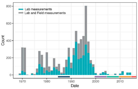
Figure 4.
Yearly histogram of the soil data—in blue, the laboratory measurements and, in grey, the laboratory and field measurements; below the graph, the considered time periods are shown.
For the soil data, we calculated the cumulative number of soil samples (locations with laboratory measurements only and locations with laboratory measurements and field estimates) that intersected with the total bare soil area of that month. This data gives an indication on the availability of soil data. As a result, the most suitable period in terms of available satellite and soil data was selected for prediction of soil properties.
3.4.2. Calibration
From the harmonised soil database, only the locations with laboratory measurements were used for calibration and validation of a multi-linear regression model. The variables, i.e., Landsat bands to include in the model, were selected based on a backward stepwise selection according to the Akaike information criterion (AIC). The best multi-linear regression model, in terms of AIC, was selected. The soil data were divided in a calibration and a validation set, of which 75% were calibration and 25% validation. The performance of the calibration dataset was quantified with a 10-fold cross validation. Based on this, we calculated the root mean square error (RMSE) and the coefficient of determination (R2). The RMSE was compared to a prediction model based on the mean of the measured soil property.
3.4.3. Validation
In order to validate the prediction performance, we predicted the soil properties for the validation dataset and calculated the corresponding RMSE and the R2. The RMSE was compared to a prediction model based on the mean of the measured soil property. Additionally, we plotted the measured versus predicted data and visually analysed the performance.
3.4.4. Visual Comparison Available Soil Maps
In order to get an impression of the potential of Bare Soil Composite for soil mapping, we compared the resulting soil property maps to available conventional and digital soil maps. For the canton of Zurich, we had a 1:5000 conventional soil map available for the agricultural area [53], and, based on the texture triangle used for this map [54], we were able to classify the polygons in five different clay classes. Additionally, for the area around the Grand Marais and the area around Zurich, we had digital soil maps available of the topsoil properties clay and soil organic matter (SOM) [55,56]. Based on this information, we did a visual comparison between the soil property prediction based on the Bare Soil Composite and the conventional and digital soil maps.
4. Results
This section follows the same structure as Chapter 3 and as Figure 2. We show the result of (A) the preprocessing steps of the satellite data including the selection of the aggregation window (Section 4.1); (B) the generation of the Barest Pixel Composite (Section 4.2); and (C) the generation of the Bare Soil Composite, including the selection of the threshold (Section 4.3). Finally, we show the result of the soil property prediction based on the Bare Soil Composite (Section 4.4).
4.1. Preprocessing
Selection of Aggregation Window
Figure 5a shows the cumulative sum of the bare soil area of five years of Landsat data for each time period (starting years 1985, 2000, 2005, 2010, and 2015). We can see that, as expected, for all time periods, the increase of bare soil area saturates with time. However, we can also see that there are fixed moments in time where the increase is stronger than the average. These moments are mainly in spring and at the end of summer, which are known to be seeding and harvest periods [16]. The exact moment is weather dependent and therefore hard to predict.
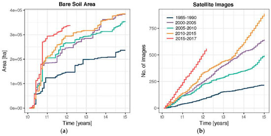
Figure 5.
Development of satellite data. The cumulative sum of the bare soil area (ha) (a) and the cumulative number of satellite images considered for the bare soil area (b) for the different time periods.
Table 3 shows the results of the fitted exponential models on these trends. The bare soil area is largest for the time period 2000 and smallest for the period 1985; however, this seems to be related to the small dataset of satellite data in this period. It is unexpected that the total area of cropland would almost double from 1985 to 2000; this is also confirmed by the land use statistics of Switzerland. In the heterogeneous agricultural area of the Swiss Plateau, it takes on average 4 years and 6 months, rounded up to 5 years, to reach 90% of the total bare soil area. These five years were selected as the aggregation window for further analysis. The variability between the periods becomes larger when getting closer to the full bare soil coverage: in order to reach 95% of the maximum area we needed, on average, 5 years and 10 months, but it fluctuated between 3 years and 1 month and 7 years and 3 months (Table 3).
Table 3.
Extrapolation results of the size of the bare soil area.
Figure 5b shows the monthly cumulative count of the number of Landsat images. The availability of the satellite data appeared more or less steady over the year. There are small fluctuations as a result of cloud cover, which is often the case in winter. However, the total amount of data (steepness of the line) changed over the years, and this can also be observed in Table 4. The period 1985–1990 is only based on L5 data, resulting in a clearly smaller dataset. The periods 2000–2005 and 2005–2010 are based a combination of L5 and L7 data. The last two time periods, 2010–2015 and 2015–2017 are also based on a combination of L7 and L8 data (from 2013 on), this is clearly visible in the steep steady line (Figure 5b); fluctuation seems to be less present.
Table 4.
Count of the satellite data used for each composite.
4.2. Barest Pixel Composite
The Barest Pixel Composite shows the true colour Red-Green-Blue (RGB) of the least vegetated pixels; for visualisation reasons, the permanently covered areas (e.g., forest, water bodies, built-up) are shown as a cloud-free greenest pixel composite. Figure 6 shows the RGB of the Barest Pixel Composite of 2000–2005. The image clearly shows more bare soils in the southwest of the Swiss Plateau, with the highest concentration around the Lakes Neuchâtel, Biel and Morat (Grand Marais). There is a general southwards pattern with decreasing bare soil area, related to the grass-dominated land cover at the foot of the Alps. In addition, towards the northeast, less bare soils are present.
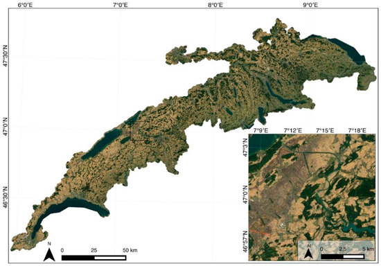
Figure 6.
Barest Pixel Composite for the time period 2000–2005 showing Landsat data (true colour Red-Green-Blue (RGB)). Pixels outside the agricultural area (e.g., water bodies, forest and built-up area) are shown as a cloud-free greenest pixel composite.
4.3. Bare Soil Composite
4.3.1. Thresholding the BSI
Table 5 shows the resulting user’s and producer’s accuracy of the bare soil class, the total accuracy and the Kappa statistic, when setting the threshold where the user’s accuracy equals the producer’s accuracy. We excluded Scene 2b because the user’s and producer’s accuracy and the kappa statistic were very low. Analysing these results, we should keep in mind that changes in bare soil can happen fast because of land management during the harvest and seeding periods or changing weather conditions, even when we took a maximum difference of three days. Furthermore, differences between the view angle of APEX and the sun elevation might also affect the threshold values (Table 2). The resulting mean of 0.021 was applied for all further analysis (i.e., values above 0.021 were considered bare soil). The variation around the mean (standard deviation 0.015) indicates that the threshold may be specific for the test site and environmental or land management conditions.
Table 5.
User’s, Producer’s, and total accuracy (%) and the Kappa statistic (%); and the corresponding threshold [-] when the User’s accuracy is equal to Producer’s accuracy.
4.3.2. Bare Soil Composite
The Bare Soil Composite shows the true colour RGB of the mean reflectance values of the bare soil pixels (defined as BSI above the 0.021 threshold). The true colour RGB of the resulting bare soil area for 2000–2005 is shown in Figure 7. The composite shows that the bare soil areas are most dominant at the north side of the Swiss Plateau and, especially in the west, just south of the Jura. Besides this, we see that the colours of the soils vary over the full area. This is an indication of the soil characteristics in the area. When we look at the zoomed area, we can clearly see a darker stripe from southwest to northeast; this area is known as the Grand Marais and its soils are high in organic matter, which are in general darker soils. Table 4 shows the amount of bare soil area of the aggregation window of five years for each time period. For the period 2000–2005, 42.9% of the agricultural area was covered by bare soils pixel, which is 30.8% of the total Swiss Plateau.
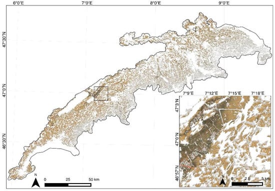
Figure 7.
Bare Soil Composite for the time period 2000–2005. Bare soil pixels are shown as true colour RGB of the Landsat data. The pixels within the agricultural area of the Swiss Plateau that showed Bare Soil Index (BSI) values below the threshold of 0.021 (e.g., grassland) are marked grey. Pixels outside the agricultural area (e.g., water bodies, forest and built-up area) are white.
4.4. Soil Property Prediction
4.4.1. Soil Data Availability
Considering the available periods of satellite data (1985–1990 and 2000–2017), most soil measurements were taken in the period 1985–1990. Appendix A shows the cumulative count of locations with laboratory measurements only (a), and locations with laboratory measurements and field estimates (b) intersecting with the bare soil area. It becomes clear from this graph that, only for the time period 1985–1990, a considerable amount of intersecting soil data is available. The other time periods show less than 100 (most of the time even less than 30) intersecting locations with in situ soil observations. However, in the 1985–1990 period, the observed bare soil area is limited because of the satellite data availability (Section 3.1.1). Therefore, we focused on the period 2000 –2005 as the best trade-off between Landsat availability and representativeness of the in situ data. For the soil property prediction, we included the soil data from the five years prior to this time period up to the end of the time period (1995–2005). This resulted in 387 soil locations for SOM and 389 for soil texture intersecting with the agricultural area.
The in situ soil data shows that the soils in the area can be on average defined as loam, but also clay loam, sandy clay loam and sandy loam soils can be found. SOM is on average 3.87% with a standard deviation of 2.59%. The summary statistics of the soil properties are shown in Table 6. These data were used for the multi-linear regression with reflectance values derived from the Bare Soil Composite.
Table 6.
Summary statistics of the soil properties.
4.4.2. Calibration
Table 7 shows the results of the 10-fold cross validation of the calibration dataset. The R2 indicates that the models for clay and SOM performed best, with R2 values of 0.22 and 0.26, respectively. The models for sand and silt performed poorly with R2 values below 0.1 and high RMSE values. For both clay and SOM, the RMSE of the regression model are, as expected, lower than the mean model. For sand and silt, on the other hand, the RMSE is above the RMSE of the mean model, which means that the mean of the soil property is a better predictor than a multi-linear model. This illustrates that the prediction of these soil parameters is not straightforward at large spatial scales. For this reason, we only show the SOM and clay prediction maps in this section.
Table 7.
Soil property prediction: results of the 10-fold cross validation of the calibration dataset and the results of the validation dataset. R2, root mean square error (RMSE), and RMSE of mean model (RMSEm) for SOM (%), clay (%), silt (%) and sand (%).
Figure 8 shows in grey the measured versus predicted soil properties of the 10-fold cross validation of the calibration dataset. These figures show clearly what was already described before. The prediction models are most stable for SOM and clay. The prediction models for sand and silt are very unstable, shown by the wide range of regression lines.
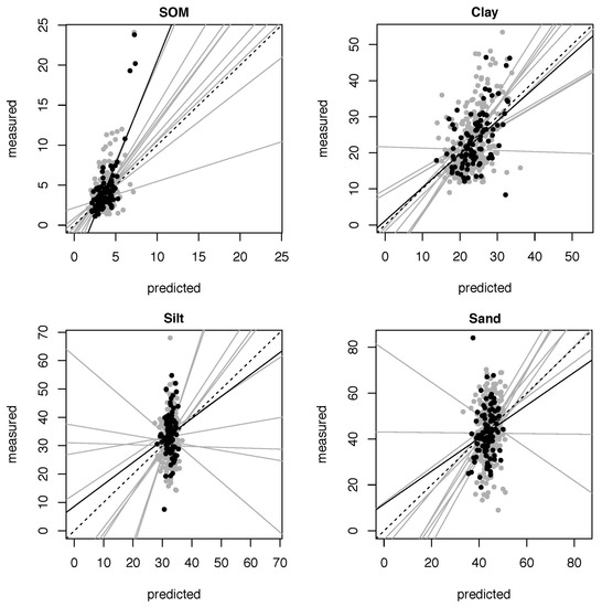
Figure 8.
Measured vs. predicted soil property values for soil organic matter (SOM), clay, silt and sand (%)—in grey, the results of the 10-fold cross validation of the calibration dataset and in black the results of the validation dataset. The dotted line shows the 1:1 line and the solid lines the multiple-linear regression lines. The corresponding R2 and root mean square error of the prediction can be found in Table 7.
Figure 9 shows the prediction results of the multi-linear regression for SOM and clay. Comparing the summary statistics of the predicted values (Table 8) with the summary statistics of the soil properties of the soil database (Table 6), we can see that the mean is very similar, the standard deviation of the predicted values is, however, much smaller. This is also emphasised by the range of the 95% percentile of the data. The range of the predicted values is much narrower than the range of the soil database. This means that high and low values are not well predicted. Patterns are similar for all soil properties. The figures of the predicted soil properties show a clear pattern for SOM and clay, which fit the geology and soil description of the Swiss Plateau (Section 2). SOM and clay are mainly high in the Grand Marais and are, in general, lower in the higher areas.
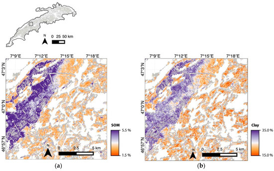
Figure 9.
Soil property maps for (a) soil organic matter (SOM) and (b) clay (%) for the time period 2000–2005. The pixels within the agricultural area of the Swiss Plateau that showed Bare Soil Index (BSI) values below the threshold of 0.021 (e.g., grassland) are marked grey. Pixels outside the agricultural area (e.g., water bodies, forest and built-up area) are white.
Table 8.
Summary statistics of the predicted soil properties. n = 4,270,458 pixels.
When we look at the multiple-linear regression equations in more detail (Table 9), we should explain the band selections for SOM and clay. For SOM, it is known that the visible part of the spectrum is often most predictive [5]. Although most of the absorption features for SOM are present in the VIS and NIR, the whole spectrum is influenced by SOM [7]. This might be the reason that the SWIR region appeared important in the regression. For clay, it is known that many absorption features can be found in the SWIR region of the spectrum [8]. The red band, on the other hand, is less clear. However, this can probably be attributed to iron and its corresponding oxidation features that are often substantially present in clayey soils [13]. For sand and silt, there are no clear absorption features in the VNIR–SWIR [57], but they are inversely related with clay. All in all, SWIR appeared a powerful spectral region in the regression analysis, as anticipated from the design of the BSI.
Table 9.
Multiple-linear equation to derive the soil properties.
4.4.3. Validation
The validation results using the validation dataset show very similar values as the performance results of the calibration dataset (Table 7). It is striking, however, that the validation dataset for SOM performs much better than the cross-validation of the calibration dataset. The R2 is 0.78 compared to the 0.26 in the cross validation and the RMSE improves much more compared to the mean model. This might have to do with the random selection of the validation dataset and the widespreadness of the SOM values of the validation dataset (Figure 8).
Figure 8 shows in black the measured versus predicted soil properties of the validation dataset. These figures show clearly what was already described before. Additionally, we can see that the patterns are well predicted for clay and SOM; however, the range of the predicted values is clearly narrower than of the measured values. For sand and silt, we have to be very careful using these prediction models, since there is no clear pattern in the regression line.
4.4.4. Visual Comparison Available Soil Maps
Figure 10 shows the comparison of the Barest Soil Composite prediction map with the available digital soil map [55,56] for predicted clay values in the area southeast of Greifensee (top) and soil organic matter (SOM) properties in northeast of the Grand Marais (bottom). For canton Zurich, the texture classes were available of the conventional soil map [53]. Comparison between the maps is possible, since all maps are based on the same legacy data (harmonised NABODAT dataset [51,52]). Nevertheless, we have to be aware of small differences. Polygons of the conventional soil map are drawn based on additional, not registered, soil samples [58], and the Barest Soil Composite map is based on the legacy soil data between 1995 and 2005 intersecting with the bare soil area of the remote sensing data.
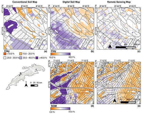
Figure 10.
Comparison between the conventional soil map (CSM), digital soil map (DSM) and the Barest Soil Composite prediction map. On top (a–c) predicted clay values (%) for the area southeast of Greifensee (area 1), respectively for the CSM, DSM and the Barest Soil Composite prediction map. The bottom (d,e) shows the predicted soil organic matter (SOM) (%) for the northeast of the Grand Marais (area 2), respectively for the DSM and the Barest Soil Composite prediction map. The conventional soil map was divided in five classes based on the texture triangle given by [59].
There are large differences between the conventional soil map and the other two maps. Some patterns are recognisable in all three maps; however, it seems that the conventional soil map does not represent the clay variation in this area very well. It is hard to say if this is related to the accuracy of the conventional soil map, or that this is related to the categorisation of the conventional soil map for clay values. The Barest Soil Composite prediction maps show very similar patterns as the digital soil map. However, the high and low values are not well predicted, the digital soil map shows, for example, much higher SOM values in the Grand Marais. A more quantitative comparison of the results would be necessary to check the performance capacities of Barest Soil Composite prediction data for soil prediction. In addition, considering that the soil predictions are only based on the six reflection bands of Landsat and already can reproduce the spatial pattern of the digital soil map, it is a promising result. Apart from this, the figure also shows that the potential of the Landsat data for soil purposes is more promising in areas with a large area of alternating crops. The area of the Grand Marais is known for its high suitability for agriculture, while the area southeast of Greifensee is less suitable for agriculture when the slopes become steeper on the northeast, this is also where soil information is missing in the Barest Soil Composite prediction.
5. Discussion and Outlook
5.1. Discussion of the Results
The results showed that, for the agricultural area of Switzerland, Landsat data could offer detailed (30 m spatial resolution) soil information between 1985 and 1990 and from 2000 until now. Although the Landsat bands have limited capacity for predicting soil properties (Section 4.4), the prediction results for SOM and clay are moderate and spatial patterns were predicted as expected. Other studies that predicted soil properties based on Landsat data [9,11,12] have shown similar or slightly better results, although comparison is difficult with only R2 as a performance indicator. Moreover, when discussing these results, we must be aware that these are exclusively based on Landsat data while most digital soil maps used many more covariates. When comparing the soil information Landsat can offer to the national soil map of Switzerland [53], it becomes clear that the property prediction may be less accurate at the in situ points, but the spatial detail is much better (results not shown). Moreover, the demonstrated method is fast and available for several time periods since 1985. Unfortunately, the digital soil information available for Switzerland is limited and mostly based on soil information from the 1990s, which makes the monitoring of changes difficult. Similarly, at the regional and global scale, soil data were mainly collected between the 1960s and 1990s [60]. With the increasing demand for full coverage soil property maps for the use in regional and global models [5], there is great potential for the use of remote sensing supporting digital soil mapping [61]. Nevertheless, the actual use of remote sensing for mapping extended areas is still limited. We are among the first, as far as we know, to show the potential of Landsat time series for the quantitative mapping of soil properties for extended areas. We conclude that the Barest Pixel Composite and the Bare Soil Composite offer valuable information for the design of sampling schemes and deriving soil properties and recommend such soil specific composites to be included in digital soil mapping efforts.
A few characteristics of the Barest Pixel Composite and the Bare Soil Composite should be carefully considered. The use of crop rotation in agricultural areas resolves the challenge of vegetation cover for temporarily covered soils. However, full coverage mapping of soils based on remote sensing data is difficult. Geostatistics and indirect correlations of soil properties with vegetation contribute to a solution (e.g., [5,62,63]), but require the development of new methods in order to retain the spatial detail that remote sensing data can offer.
Within agricultural areas, the nature of what is considered as bare soil is not always clear. These may, for instance, be natural (unmanaged bare soil), artificial (e.g., construction) or crop rotation. Although the bare soil in our study area is dominantly the result of crop rotation, it is possible that confusion with other types exist. Depending on the application, this might affect the results. Furthermore, we selected the observation dates (and thus reflectance values) based on the mean above the BSI threshold of 0.021. However, the threshold may be site or soil specific and determining it requires field observations or expert interpretation of the imagery. Using the maximum BSI value (and thus the Barest Pixel Composite instead of the Bare Soil Composite) has the advantage of its universal applicability: the Barest Pixel Composite can be calculated for any region and period with a sufficient Landsat coverage. On the other hand, taking the mean BSI above a certain threshold and the mean of the corresponding Landsat bands (i.e., the Bare Soil Composite) reduces the sensitivity to anomalous observations or conditions and gives as such a more realistic picture of the mean bare soil conditions. For this reason, we have selected this approach for the soil property prediction. In this study, we based the prediction of soil properties for the time period 2000–2005 on the soil data from 1995–2005. This means that a large part of the data was excluded from the prediction model. Depending on the purpose of the prediction, it might be better to include all soil data. However, when considering that soil properties may change over longer time periods (e.g., decades), the selection of a limited time period will better represent the soil properties of this time period. For monitoring reasons, we decided to select the 1995–2005 period. When including all soil data (SOM: n = 1473; clay, sand and silt: n = 1525), the prediction performance increased marginally (Appendix B, Table A1).
5.2. Variability of the Results
We get an idea of the variability of the used Landsat data over time when we predict the soil properties for each moment in time that a pixel was bare (BSI > 0.021). Figure 11 shows the predicted soil property variability for SOM and clay over time for a single pixel in the Grand Marais. It is clear that the variability over time is high and that the deviation from the mean can be large, especially in the recent time periods (2010–2015 and 2015–2017). This variability can be caused by differences between the Landsat sensors, including differences in atmospheric correction, differences between the bands, or differences in view angle. Additionally, the variability can be caused by differences in weather conditions and land management in the different time periods cause differences in soil moisture and soil surface roughness, which both influence the surface reflectance of the soil (also discussed in Diek et al. [16]). Using the mean over the time periods reduces the variability; however, as Figure 11 shows, the bareness frequency changes for each time period.
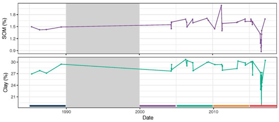
Figure 11.
Variability of soil organic matter (SOM) (top) and clay (bottom) over time for a single pixel in the Grand Marais (47°01′07.2′′N, 7°11′26.0′′E). Multi-linear regression functions of Table 9 were applied to each moment in time the considered pixel was bare. The grey block is indicating the time period 1990–2000, which was excluded because of limited available Landsat data. Below the different aggregation windows are indicated (blue: 1985–1990; purple: 2000–2005; green: 2005–2010; orange: 2010–2015; red: 2015–2017).
The variability for a single pixel is relatively easy to interpret. However, when we do a similar analysis for the focus area used in Figure 6, Figure 7 and Figure 8, it becomes more difficult to interpret the results. Figure 12 shows the variability over time for the mean SOM and clay values of the focus area. It is possible to observe a seasonal change, where values for SOM and clay are high in winter and low in summer. Since these soil properties do not change in such a short time period, this variability can be most probably related to soil moisture, which is higher in winter and lower in summer. Moreover, this figure could also be used for monitoring of soil properties over time–for example, for SOM, we can see a small increase over time. However, the interpretation of this figure should be done with care because the amount of pixels the calculation is based on varies over time. This is shown in the bar plot on top of the figure, which shows the percentage of pixels that are taken into account for the calculation of the mean soil property.
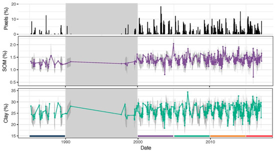
Figure 12.
Variability of the mean soil organic matter (SOM) (middle) and clay (bottom) values over time for the focus area used in Figure 6, Figure 7 and Figure 8, located in the Grand Marais. Multi-linear regression functions of Table 9 were applied to each moment in time for all bare soil pixels in the focus area. The grey area around the mean values indicate the standard deviation of the soil properties. The grey block is indicating the time period 1990–2000, which was excluded because of limited available Landsat data. Below the different aggregation windows are indicated (blue: 1985–1990; purple: 2000–2005; green: 2005–2010; orange: 2010–2015; red: 2015–2017). The bar plot on top shows the percentage of the focus area that were bare and taken into account for the calculation of the mean and standard deviation.
5.2.1. Differences between Sensors
Although the bands of each sensor cover similar spectral regions, they are not exactly the same (Table 1). This means that using composites based on a combination of data of several sensors can result in uncertainties. Additionally, differences in atmospheric correction and view angle between sensors can result in differences between the sensors. We compared several overlapping scenes of different sensors that were acquired within 24 h from each other to study this potential uncertainty. We did this for the individual reflectance bands of Landsat, for the derived BSI values and for the derived soil properties (Table 10, the mean of the considered pixel values can be found in Appendix C, Table A2). Some of the variation may be attributed to different acquisition conditions (e.g., rain events, land management, etc.), although the scenes were taken within 24 h from each other.
Table 10.
R2 of the linear regression, root mean square error (RMSE) and Mean Error between the bands of Landsat 5 TM vs. Landsat 7 ETM+ (L5L7) and Landsat 7 ETM+ vs. Landsat 8 OLI (L7L8), the derived bare soil index (BSI) and the derived soil properties. L5L7 reflectance bands and BSI: n = 8,027,616; soil properties: n = 71,987; L7L8 reflectance bands and BSI: n = 7,868,682; soil properties: n = 106,114.
For the spectral bands, the RMSE results were slightly lower than what [64] reported. However, the mean error was in general smaller for the VIS reflectance bands, but bigger for the NIR and SWIR region; and the R2 values were lower for the VIS reflectance bands. This might be related to the focus on the agricultural area, which reduces the range of the reflectance data, especially in the VIS range. For the derived BSI values, the results were very good (high R2 values). RMSE and mean error were low, which means that the influence on the BSI is small. Differences were slightly larger between L7 and L8. For the derived soil properties, the results were also good (high R2 values). Differences were especially small for silt and SOM, which both seemed least influenced by the differences of the sensors. For sand and clay, there was a more clear deviation from the 1:1 line, especially for L5L7 (positive mean error, bias towards L5).
In conclusion, the differences between Landsat sensors may have influenced the results of, especially, the soil property predictions but less the Landsat composite products. Biases are in general small, which makes it extremely difficult to correct for the biases. Taking the mean of the reflectance values over time further reduces the differences between sensors.
5.2.2. Differences in Temporal Coverage
The revisit time of Landsat satellites depends on the overlap between paths or rows and is not everywhere the same. Figure 13 shows the temporal coverage of the Landsat data for the Swiss Plateau for the 2000–2005 time period. Three southwest to northeast strips regions were clearly less covered than the rest of the Swiss Plateau. On the other hand, two west–east oriented strips show a higher coverage, probably due to overlap between consecutive Landsat images. These overlapping rows provide little additional information in comparison to overlapping paths because the images are acquired with minimal time difference and therefore largely under identical environmental and weather conditions. When we zoom in and look at the number of pixels that were actually classified as bare soil in this period, we can see a large variation. The temporal coverage is not only dependent on the Landsat coverage, but also on the weather conditions, the crop type and the land management system.
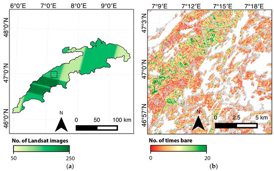
Figure 13.
Temporal coverage for the time period 2000-2005 of Landsat images for the full Swiss Plateau (a) and the number of times a pixel is classified as bare soil (BSI > 0.021) in the focus area (b).
5.2.3. Differences in Soil Moisture
It is known that soil moisture affects the reflectance data, and this effect was first described by [65]. The main effect is the increasing reflectance with decreasing soil moisture. Some spectral features are more affected [6], especially the water absorption features around 1400 and 1900 nm and the SWIR range [66,67,68]. As a result, soil moisture tends to mask the effect of other soil properties (e.g., organic matter and iron oxides) [69]. Compositing data from different dates, like in the Barest Pixel Composite and in the Bare Soil Composite, results in a great variation of soil moisture. This might affect the derived soil properties.
The BSI was tested for its sensitivity to differences in soil moisture based on an independent dataset (results not shown) and based on a soil moisture index applied on the Landsat data (methodology described in Appendix D.1) The results showed no correlation between the BSI and soil moisture (Figure 14). In this study, the bare soil selection is based on the highest BSI (Barest Pixel Composite) or the mean BSI above a certain threshold (Bare Soil Composite). Therefore, the results indicate that the bare soil pixel selection is not influenced directly by soil moisture (i.e., no biased selection towards only wet or dry pixels). Nevertheless, we can anticipate that some areas have been acquired under drier or wetter conditions than others. This may influence the result of the Bare Soil Composite and particularly the prediction of the soil properties. This effect is demonstrated by the results in Appendix D.2. Especially, clay and sand showed a certain co-variation with soil moisture, positive and negative, respectively. The water holding capacity of clay may partly explain this: soil with more clay, and thus less sand and/or silt, hold more water and the other way around. This is similar for SOM because it is known that soils with more SOM hold more water [70]. The effect of soil moisture can be spectrally corrected but existing methods (e.g., [67,71,72,73,74,75]) were developed for imaging spectroscopy data and are not easily applicable to multispectral data. Soil surface roughness also affects the reflectance of a bare soil. The effects are similar to the effect of soil moisture on reflectance, but are less severe and more linear over the spectrum [72]. In general, an increase of soil surface roughness leads to a decrease in reflectance values, mainly as a result of shadow [76]. It is almost impossible to estimate this effect from Landsat data and correct for it. The impact can be expected to be low, especially for observations with a bigger spatial resolution and a high solar angle that results in fewer shadows.
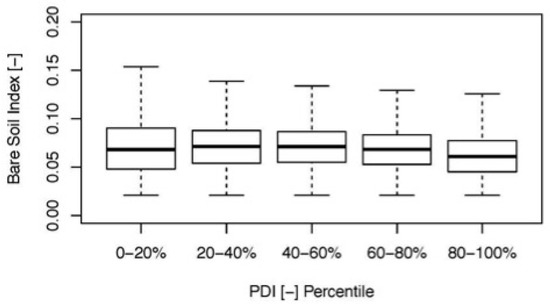
Figure 14.
Effect of soil moisture (perpendicular drought index (PDI) [-]; low values indicate a high soil moisture, high values a low soil moisture) on the bare soil index (BSI) [-]. Outliers were excluded from the figure because of visualisation reasons.
5.3. Outlook
5.3.1. Potential for Upscaling
There is a clear potential to upscale this information to national, European or even global scale. Similar upscaling to global scale was recently done for forest [77] and for surface water bodies [78]. Main condition is that agricultural fields are bare after harvesting and/or before seeding, which may not be the case everywhere. Other auxiliary data than used in this study is necessary for masking forest, built-up, water and natural areas. For European scale, candidates are the Hansen Global Forest Change dataset [77] for forest and for water, wetlands, natural grassland and built-up it is possible to use data from the Copernicus Land Monitoring Service, respectively, the Permanent Water Bodies dataset, the Wetlands dataset, the Natural Grassland dataset, and the Imperviousness dataset. All datasets are available in 20 and 100 m resolution. For global scale, the same data may be used for masking forest. For water, the JRC Global Surface Water Mapping Layers [78] are available and for built-up the Global Urban Footprint [79]. There are no readily available sources for masking natural (vegetated) areas at high spatial resolution and global extent but available land-cover products provide feasible alternatives. Soil properties could be predicted based on Harmonized Global Soil Profile Dataset (HGSPD [80]). The HGSPD is one of the global datasets used to create the Harmonized World Soil Database (HWSD [81]) and consists of 10,250 soil profiles, with some 47,800 horizons, from 149 countries. The dataset contains, however, several extended areas with lacking or a very low sampling density and the profiles are not uniformly sampled, described, and analysed, but vary according to methods and standards in use in the originating countries.
As a demonstration, we calculated the Barest Pixel and Bare Soil Composites for Europe for the time period 2010–2015. This resulted in a collection of 69,746 Landsat scenes (12,183 L5; 35,535 L7; 22,028 L8). As an indication of the processing efforts, the Barest Pixel Composite of Europe (Figure 15) with a resolution of 30 m. Furthermore, 30 GB in size and required ca. 30 h of processing time on the Earth Engine platform.
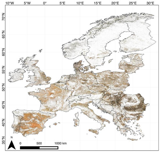
Figure 15.
RGB of the Bare Soil Composite for the whole of Europe (60 m resolution). The pixels within the agricultural area of Europe that showed Bare Soil Index (BSI) values above the threshold of 0.021 (e.g., grassland) are marked grey. Pixels outside the agricultural area (e.g., water bodies, forest and built-up area) are white. Iceland has been excluded from this composite because of insufficient Landsat coverage.
5.3.2. Application Potential
Products like the Barest Pixel Composite or the Bare Soil Composite have many more applications than the prediction of soil properties. Alternative applications are mainly of interest for land management modelling and policymaking. In this section, we list a few products that can be derived from the Barest Pixel Composite.
Based on the assumption that the alternation between bare soil and vegetation indicates crop rotation, it is possible to distinguish between cropland and grassland within the agricultural area (i.e., a pixel is considered cropland when the pixel has been bare at least once in the considered time period). This is of great value for land management modelling, mainly because these data are not always publicly available [20].
Information of the BSI over time can give us information on when croplands are bare, how often and how long. This information is useful, especially in Switzerland, where policies enforce full year coverage of soils in order to prevent soil erosion.
We can even make a step further by including NDVI and gain information on types of land management. The moment of bare soil and the development of the NDVI over time can give us information on when crops were seeded and harvested. With relative simple logic, it is possible to classify winter crops, summer cops and grasslands. Summer crops have a short growing season, NDVI peak in late summer, are seeded in spring, and harvested in autumn; winter crops have a longer growing season, NDVI peak early summer, are seeded in autumn, and harvested late summer; grasslands are always vegetated and have small fluctuations in NDVI. An example of this is shown in Figure 16. The different combinations of certain crops over the period of crop rotation can give information on the land management type of the field. Such an analysis could be complemented with the research done by Thenkabail et al. (e.g., [82]) and Ozdogan et al. (e.g., [83]), who focus on the use of remote sensing in order to distinguish irrigated agriculture.
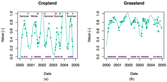
Figure 16.
Normalised difference vegetation index (NDVI) and the BSI time series for cropland (a) and grassland (b). The NDVI is shown with the green dots, the green line is a fitted spline model. The BSI (after thresholding) is shown in purple dots, where 0 is vegetated and 1 is bare soil. Based on the NDVI fluctuations and the moments of bare soil, we can classify summer crops (short growing season, peak in late summer, seeding in spring, harvest in autumn) and winter crops (longer growing season, peak early summer, seeding in autumn, harvest late summer).
6. Conclusions
This study shows that Landsat time series from 1985 to 2017 (excluding 1990–2000 because of limited availability of Landsat data) can be used to create a Barest Pixel Composite, from which soil properties can be derived. For a full coverage Bare Soil Composite, in a heterogeneous agricultural area like the Swiss Plateau in Switzerland, ca. 5 years of Landsat data were required to cover 90% of the total bare soil area. Clay fraction and soil organic matter could be derived from this Bare Soil Composite and may be used as additional data sources to traditional soil maps. Furthermore, prediction results were promising, in particular given the singular data source. Moreover, our method is computationally fast and available for several time periods since 1985. The composites further offer potential for use in land management modelling and can be up-scaled to European or global level. We conclude that the Barest Pixel Composite and the Bare Soil Composite offer valuable information for the design of soil sampling schemes as well as deriving soil properties. It is highly desirable that such soil-specific composites will be included in digital soil mapping in the near future.
Acknowledgments
This study was funded by the Swiss National Science Foundation (SNSF) and the Bundesamt für Umwelt (BAFU) in the frame of the National Research Programme “Sustainable use of Soil as a Resource” (NRP 68). Within the NRP 68, the study was part of the project “Predictive mapping of soil properties for the evaluation of soil functions at regional scale” (www.nfp68.ch). The contribution of M.E.S. is supported by the University of Zurich Research Priority Program on “Global Change and Biodiversity” (URPP GCB). APEX data acquisition was supported by the Swiss Earth Observatory Network (http://www.seon.uzh.ch) project. We would like to thank the people who harmonised the NABODAT dataset (https://nabodat.ch).
Author Contributions
F.F. and S.D. designed the research and analysed the data with scientific advice of R.d.J. and M.E.S. S.D. wrote the manuscript, R.d.J. reviewed and edited the manuscript in detail and all other co-authors thoroughly reviewed and edited the manuscript.
Conflicts of Interest
The authors declare no conflict of interest. The founding sponsors had no role in the design of the study; in the collection, analyses, or interpretation of data; in the writing of the manuscript, and in the decision to publish the results.
Abbreviations
The following abbreviations are used in this manuscript:
| AIC | Akaike information criterion |
| APEX | Airborne Prism Experiment |
| BSI | Bare Soil Index |
| CL | cropland |
| CLGL | cropland to grassland |
| GEE | Google Earth Engine |
| GL | grassland |
| GLCL | grassland to cropland |
| L5 | Landsat-5 Thematic Mapper |
| L7 | Landsat-7 Enhanced Thematic Mapper+ |
| L8 | Landsat-8 Operational Land Imager |
| MSS | multispectral scanner |
| nCAI | normalised cellulose absorption index |
| NDBI | normalised difference built-up index |
| NDRBI | normalised difference red blue index |
| NDSI | normalised difference snow index |
| NDVI | normalised difference vegetation index |
| NIR | near-infrared |
| PDI | perpendicular drought index |
| RMSE | root mean square error |
| SL | soil line |
| SLC | scan line corrector |
| SOM | soil organic matter |
| SR | surface reflectance |
| SWIR | shortwave-infrared |
| TIR | thermal infrared |
| TM | Thematic Mapper |
| VIS | visible |
| VNIR-SWIR | visible, near- and shortwave-infrared |
Appendix A. Intersecting Lab and Field Data over Time
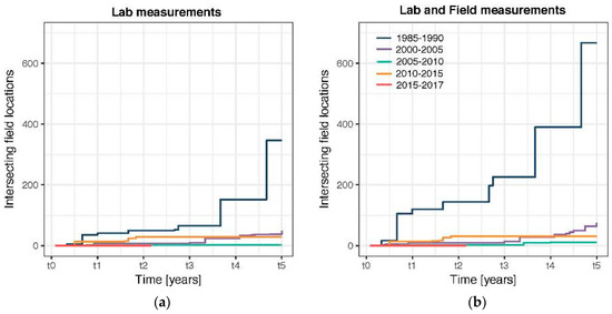
Figure A1.
Development of the soil data over time. The cumulative sum of the laboratory measurements intersecting with the bare soil area (a) and the laboratory and field measurements intersecting with the bare soil area (b).
Appendix B. Soil Property Prediction Based on All Soil Data
Table A1.
Soil property prediction: 10-fold cross validation results. R2, RMSE and RMSE of mean model (RMSEm) for SOM (%), clay (%), silt (%) and sand (%).
Table A1.
Soil property prediction: 10-fold cross validation results. R2, RMSE and RMSE of mean model (RMSEm) for SOM (%), clay (%), silt (%) and sand (%).
| Property | n 1 | R2 (-) | RMSE (%) 2 | RMSEm (%) |
|---|---|---|---|---|
| SOM | 1473 | 0.27 ± 0.14 | 2.83 ± 0.50 | 3.26 ± 0.62 |
| Clay | 1525 | 0.18 ± 0.06 | 8.05 ± 0.46 | 8.90 ± 0.48 |
| Silt | 1525 | 0.02 ± 0.03 | 7.25 ± 0.73 | 7.29 ± 0.70 |
| Sand | 1525 | 0.09 ± 0.04 | 11.60 ± 0.96 | 12.01 ± 0.86 |
1 number of observations; 2 RMSE: root mean square error.
Appendix C. Mean L5L7 and L7L8
Table A2.
Mean of the bands of Landsat 5 TM vs. Landsat 7 ETM+ (L5L7) and Landsat 7 ETM+ vs. Landsat 8 OLI (L7L8). L5L7 reflectance bands and BSI: n = 8,027,616; soil properties: n = 71,987; L7L8 reflectance bands and BSI: n = 7,868,682; soil properties: n = 106,114.
Table A2.
Mean of the bands of Landsat 5 TM vs. Landsat 7 ETM+ (L5L7) and Landsat 7 ETM+ vs. Landsat 8 OLI (L7L8). L5L7 reflectance bands and BSI: n = 8,027,616; soil properties: n = 71,987; L7L8 reflectance bands and BSI: n = 7,868,682; soil properties: n = 106,114.
| L5L7 | L7L8 | |||
|---|---|---|---|---|
| Mean L5 | Mean L7 | Mean L7 | Mean L8 | |
| Blue | 4.91 ± 2.71 | 5.02 ± 2.41 | 4.71 ± 2.08 | 3.83 ± 2.74 |
| Green | 7.95 ± 2.40 | 7.69 ± 2.70 | 6.94 ± 2.34 | 7.03 ± 2.98 |
| Red | 6.86 ± 3.24 | 6.51 ± 3.85 | 6.43 ± 3.41 | 6.53 ± 4.03 |
| NIR | 35.30 ± 9.56 | 37.20 ± 9.38 | 31.76 ± 10.61 | 33.33 ± 11.03 |
| SWIR1 | 19.85 ± 5.33 | 20.82 ± 5.77 | 19.71 ± 6.16 | 20.38 ± 6.51 |
| SWIR2 | 11.35 ± 5.11 | 11.58 ± 5.55 | 11.21 ± 5.08 | 12.34 ± 5.48 |
| BSI | −0.38 ± 0.21 | −0.41 ± 0.22 | −0.35 ± 0.22 | −0.33 ± 0.23 |
| SOM 1 | 3.35 ± 1.47 | 3.23 ± 1.55 | 4.42 ± 2.16 | 4.58 ± 3.21 |
| Clay | 22.33 ± 7.38 | 19.26 ± 7.48 | 25.05 ± 7.95 | 23.40 ± 9.36 |
| Silt | 32.77 ± 2.06 | 33.15 ± 2.54 | 32.44 ± 2.26 | 32.54 ± 2.70 |
| Sand | 45.87 ± 5.59 | 48.49 ± 5.36 | 43.96 ± 6.12 | 45.61 ± 7.19 |
1 SOM: soil organic matter.
Appendix D. Effect of Soil Moisture
Appendix D.1. Methodology
In order to look at the influence of soil moisture on the prediction of soil properties, we calculated a soil moisture index. We used the perpendicular drought index (PDI) [84] as soil moisture index, defined in Equation (A1). The methodology of the PDI is based on the methodology described by Richardson and Wiegand [85]:
where and are the surface reflectance for, respectively, the red and the NIR bands and is the slope of the soil line. The PDI is based on the NIR-Red spectral space, in which a triangle is formed when plotting the NIR and red reflectance of vegetated and non-vegetated pixels under variable soil moisture conditions. Figure A2 shows this NIR-Red spectral space, where the triangular area represents the change of surface vegetation from full coverage (top triangle) to partial coverage to bare soil (bottom triangle). The base line of the triangle refers to the soil line, which shows the bare soil reflectance from wet conditions, to semi-arid conditions to extremely dry conditions, based on Figure 1 of [86]. A global soil line (SL) was defined by [87], based on five different studies containing different soil types (Equation (A2) and Figure A2). Figure A2 shows that this global soil line is also applicable to the agricultural area of the Swiss Plateau:
Consequently, the PDI values for the agricultural area were divided in five soil moisture classes, based on the distribution of the data. For this, we used the 5 percentiles (0–20%, 20–40%, 40–60%, 60–80% and 80–100%). Because of the large amount of pixels, the soil moisture classes make the results easier to interpret.
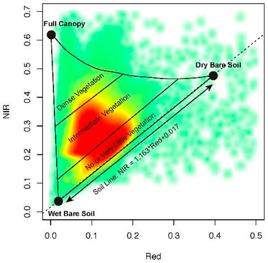
Figure A2.
Soil Line (SL) for the Barest Pixel Composite of the agricultural area of the Swiss Plateau and the theory of the NIR-red triangle space [86]. The scatterplot is shown as a density plot, ranging from green to red (little points to many points).
Appendix D.2. Effect of Soil Moisture on Soil Property Prediction
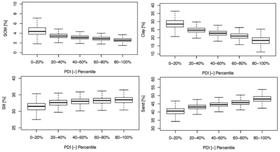
Figure A3.
Effect of soil moisture (perpendicular drought index (PDI) [-]; low values indicate a high soil moisture, high values a low soil moisture) on the soil property prediction (soil organic matter (SOM, clay, silt and sand [%]). Outliers were excluded from the figure, because of visualisation reasons.
References
- Breure, A.M.; De Deyn, G.B.; Dominati, E.; Eglin, T.; Hedlund, K.; Van Orshoven, J.; Posthuma, L. Ecosystem services: A useful concept for soil policy making! Curr. Opin. Environ. Sustain. 2012, 4, 578–585. [Google Scholar] [CrossRef]
- Banwart, S. Save our soils. Nature 2011, 474, 151–152. [Google Scholar] [CrossRef] [PubMed]
- Godfray, H.C.J.; Beddington, J.R.; Crute, I.R.; Haddad, L.; Lawrence, D.; Muir, J.F.; Pretty, J.; Robinson, S.; Thomas, S.M.; Toulmin, C. The Challenge of Food Security. Science 2012, 327, 812. [Google Scholar] [CrossRef] [PubMed]
- Dewitte, O.; Jones, A.; Elbelrhiti, H.; Horion, S.; Montanarella, L. Satellite remote sensing for soil mapping in Africa. Prog. Phys. Geogr. 2012, 36, 514–538. [Google Scholar] [CrossRef]
- Mulder, V.L.; de Bruin, S.; Schaepman, M.E.; Mayr, T.R. The use of remote sensing in soil and terrain mapping—A review. Geoderma 2011, 162, 1–19. [Google Scholar] [CrossRef]
- Ben-Dor, E.; Chabrillat, S.; Demattê, J.A.M.; Taylor, G.R.; Hill, J.; Whiting, M.L.; Sommer, S. Using imaging spectroscopy to study soil properties. Remote Sens. Environ. 2009, 113, S38–S55. [Google Scholar] [CrossRef]
- Nocita, M.; Stevens, A.; van Wesemael, B.; Aitkenhead, M.; Bachmann, M.; Barthès, B.G.; Ben-Dor, E.; Brown, D.J.; Clairotte, M.; Csorba, A.; et al. Soil Spectroscopy: An Alternative to Wet Chemistry for Soil Monitoring. Adv. Agron. 2015, 132, 139–159. [Google Scholar] [CrossRef]
- Soriano-Disla, J.M.; Janik, L.J.; Viscarra Rossel, R.A.; MacDonald, L.M.; McLaughlin, M.J. The performance of visible, near-, and mid-infrared reflectance spectroscopy for prediction of soil physical, chemical, and biological properties. Appl. Spectrosc. Rev. 2014, 49, 139–186. [Google Scholar] [CrossRef]
- Demattê, J.A.M.; Galdos, M.V.; Guimarães, R.V.; Genú, A.M.; Nanni, M.R.; Zullo, J., Jr.; Zullo, J. Quantification of tropical soil attributes from ETM+/LANDSAT-7 data. Int. J. Remote Sens. 2007, 28, 3813–3829. [Google Scholar] [CrossRef]
- Nanni, M.R.; Demattê, J.A.M.; Chicati, M.L.; Fiorio, P.R.; Cézar, E.; De Oliveira, R.B. Soil surface spectral data from landsat imagery for soil class discrimination. Acta Sci. Agron. 2012, 34, 103–112. [Google Scholar] [CrossRef]
- Shabou, M.; Mougenot, B.; Chabaane, Z.; Walter, C.; Boulet, G.; Aissa, N.; Zribi, M. Soil Clay Content Mapping Using a Time Series of Landsat TM Data in Semi-Arid Lands. Remote Sens. 2015, 7, 6059–6078. [Google Scholar] [CrossRef]
- Fiorio, P.R.; Demattê, J.A.M. Orbital and laboratory spectral data to optimize soil analysis. Sci. Agric. 2009, 66, 250–257. [Google Scholar] [CrossRef]
- Ben-Dor, E.; Irons, J.R.; Epema, G.F.; Ryerson, R.A. Soil Reflectance. In Remote Sensing for the Earth Sciences; Rencz, A.N., Ed.; John Wiley & Sons, Inc.: Hoboken, NJ, USA, 1999; pp. 111–188. ISBN 0471-29405-5. [Google Scholar]
- Gerighausen, H.; Menz, G.; Kaufmann, H. Spatially explicit estimation of clay and organic carbon content in agricultural soils using multi-annual imaging spectroscopy data. Appl. Environ. Soil Sci. 2012, 2012. [Google Scholar] [CrossRef]
- Demattê, J.A.M.; Alves, M.R.; Terra, F.D.S.; Bosquilia, R.W.D.; Fongaro, C.T.; Barros, P.P.D.S. Is it possible to classify topsoil texture using a sensor located 800 km away from the surface? Rev. Bras. Cienc. Solo 2016, 40, 1–13. [Google Scholar] [CrossRef]
- Diek, S.; Schaepman, M.E.; de Jong, R. Creating multi-temporal composites of airborne imaging spectroscopy data in support of digital soil mapping. Remote Sens. 2016, 8, 906. [Google Scholar] [CrossRef]
- Google Earth Engine Team Google Earth Engine: A Planetary-Scale Geospatial Analysis Platform. Available online: https://earthengine.google.com (accessed on 26 July 2017).
- Padarian, J.; Minasny, B.; McBratney, A.B. Using Google’s cloud-based platform for digital soil mapping. Comput. Geosci. 2015, 83, 80–88. [Google Scholar] [CrossRef]
- Eidgenössisches Departement für Auswärtige Angelegenheiten Swiss Plateau. Available online: https://www.eda.admin.ch/aboutswitzerland/en/home/umwelt/geografie/mittelland.html (accessed on 28 June 2017).
- Gomez Gimenez, M.; Della Peruta, R.; de Jong, R.; Keller, A.; Schaepman, M.E. Spatial Differentiation of Arable Land and Permanent Grassland to Improve a Land Management Model for Nutrient Balancing. IEEE J. Sel. Top. Appl. Earth Obs. Remote Sens. 2016, 9. [Google Scholar] [CrossRef]
- Gnägi, C.; Labhart, T.P. Geologie der Schweiz; Hep Verlag: Bern, Switzerland, 2015; ISBN 978-3-7225-0142-0. [Google Scholar]
- Frei, E.; Peyer, K. Übersicht 1:500,000. In Atlas der Schweiz; Spies, E., Ed.; Bundesamt für Landestopographie: Bern, Switzerland, 1984. [Google Scholar]
- United States Geological Survey (USGS). Landsat Missions Timeline. Available online: https://landsat.usgs.gov/landsat-missions-timeline (accessed on 28 June 2017).
- United States Geological Survey (USGS). Landsat 7. Available online: https://landsat.usgs.gov/landsat-7 (accessed on 28 June 2017).
- United States Geological Survey (USGS). What Are the Band Designations for the Landsat Satellites? Available online: https://landsat.usgs.gov/what-are-band-designations-landsat-satellites (accessed on 28 June 2017).
- United States Geological Survey (USGS). Geometry. Available online: https://landsat.usgs.gov/geometry (accessed on 24 October 2017).
- Hall, D.K.; Riggs, G.A.; Salomonson, V.V. Development of methods for mapping global snow cover using moderate resolution imaging spectroradiometer data. Remote Sens. Environ. 1995, 54, 127–140. [Google Scholar] [CrossRef]
- Piyoosh, A.K.; Ghosh, S.K. Development of a modified bare-soil and urban index for Landsat 8 satellite data. Geocarto Int. 2017. [Google Scholar] [CrossRef]
- Rouse, J.W.; Haas, R.H.; Deering, D.W. Monitoring vegetation systems in the Great Plains with ERTS. Third ERTS Symp. 1973, 1, 309–317. [Google Scholar]
- Tucker, C.J. Red and photographic infrared linear combinations for monitoring vegetation. Remote Sens. Environ. 1979, 8, 127–150. [Google Scholar] [CrossRef]
- He, C.; Shi, P.; Xie, D.; Zhao, Y. Improving the normalized difference built-up index to map urban built-up areas using a semiautomatic segmentation approach. Remote Sens. Lett. 2010, 1, 213–221. [Google Scholar] [CrossRef]
- Zha, Y.; Gao, J.; Ni, S. Use of normalized difference built-up index in automatically mapping urban areas from TM imagery. Int. J. Remote Sens. 2003, 24, 583–594. [Google Scholar] [CrossRef]
- Stathakis, D.; Perakis, K.; Savin, I. Efficient segmentation of urban areas by the VIBI. Int. J. Remote Sens. 2012, 33, 6361–6377. [Google Scholar] [CrossRef]
- Rikimaru, A.; Roy, P.S.; Miyatake, S. Tropical forest cover density mapping. Trop. Ecol. 2002, 43, 39–47. [Google Scholar]
- Deka, J.; Tripathi, O.P.; Khan, M.L. Implementation of Forest Canopy Density Model to Monitor Tropical Deforestation. J. Indian Soc. Remote Sens. 2013, 41, 469–475. [Google Scholar] [CrossRef]
- Jamalabad, M.; Abkar, A.A. Forest canopy density monitoring, using satellite images. In Proceedings of the Geo-Imagery Bridging Continents XXth ISPRS Congress, Istanbul, Turkey, 12–23 July 2004; pp. 12–23. [Google Scholar]
- Chen, W.; Liu, L.; Zhang, C.; Wang, J.; Wang, J.; Pan, Y. Monitoring the seasonal bare soil areas in beijing using multi-temporal TM images. In Proceedings of the 2004 IEEE International Geoscience and Remote Sensing Symposium, Anchorage, AK, USA, 20–24 September 2004; pp. 3379–3382. [Google Scholar]
- Zhao, H.; Chen, X. Use of normalized difference bareness index in quickly mapping bare areas from TM/ETM+. In Proceedings of the 2005 IEEE International Geoscience and Remote Sensing Symposium, Seoul, Korea, 29 July 2005; pp. 1666–1668. [Google Scholar] [CrossRef]
- Kawamura, M.; Jayamanna, S.; Tsujiko, Y. Relation between social and environmental conditions in Colombo Sri Lanka and the urban index estimated by satellite remote sensing data. Int. Arch. Photogramm. Remote Sens. 1996, 31, 321–326. [Google Scholar]
- Bundesamt für Landestopografie Swisstopo. Landeskarte 1:25000. 2008. Available online: https://shop.swisstopo.admin.ch/en/products/maps/national/lk25 (accessed on 26 July 2017).
- Schaepman, M.E.; Jehle, M.; Hueni, A.; D’Odorico, P.; Damm, A.; Weyermann, J.J.; Schneider, F.D.; Laurent, V.C.E.; Popp, C.; Seidel, F.C.; et al. Advanced radiometry measurements and Earth science applications with the Airborne Prism Experiment (APEX). Remote Sens. Environ. 2015, 158, 207–219. [Google Scholar] [CrossRef]
- Chabrillat, S.; Eisele, A.; Guillaso, S.; Rogaß, C.; Ben-Dor, E.; Kaufmann, H. HYSOMA: An easy-to-use software interface for soil mapping applications of hyperspectral imagery. In Proceedings of the 7th EARSeL SIG Imaging Spectroscopy Workshop, Edinburgh, UK, 11–13 April 2011. [Google Scholar]
- Carter, G.A. Primary and secondary effects on water content on the spectral reflectance of leaves. Am. J. Bot. 1991, 78, 916–924. [Google Scholar] [CrossRef]
- Zakaluk, R.; Sri Ranjan, R. Predicting the leaf water potential of potato plants using RGB reflectance. Can. Biosyst. Eng. 2008, 50, 7.1–7.12. [Google Scholar]
- Nagler, P.L.; Inoue, Y.; Glenn, E.P.; Russ, A.L.; Daughtry, C.S.T. Cellulose absorption index (CAI) to quantify mixed soil-plant litter scenes. Remote Sens. Environ. 2003, 87, 310–325. [Google Scholar] [CrossRef]
- Bundesamt für Landestopografie Swisstopo. Feldblockkarte zum Erosionsrisiko. 2014. Available online: https://data.geo.admin.ch/ch.blw.feldblockkarte/ (accessed on 26 July 2017).
- Bundesamt für Landestopografie Swisstopo. swissBUILDINGS3D 1.0. 2014. Available online: https://shop.swisstopo.admin.ch/en/products/landscape/build3D (accessed on 26 July 2017).
- Bundesamt für Landestopografie Swisstopo. swissTLM3D. 2014. Available online: https://shop.swisstopo.admin.ch/en/products/landscape/tlm3D (accessed on 26 July 2017).
- Bonnard, L.F. Soil Survey in Switzerland, 2nd ed.; Jones, R.J.A., Housková, B., Bullock, P., Montanarella, L., Eds.; European Soil Bureau, Institute for Environment & Sustainability, JRC: Ispra, Italy, 2005. [Google Scholar]
- Frei, E.; Vökt, U.; Flückiger, H.; Brunner, H.; Schai, F. Bodeneignungskarte der Schweiz, Massstab 1:200000; Grundlagen für die Raumplanung, Bundesämter für Raumplanung, Landwirtschaft und Forstwesen; EDMZ: Bern, Switzerland, 1980. [Google Scholar]
- Rehbein, K.; van der Meer, M.; Grob, U.; Wegmann, F.; Keller, A. Das Nationale Bodeninformationssystem NABODAT in der Schweiz. In Proceedings of the Jahrestagung Deutschen Bodenkundlichen Gesellschaft, Berlin/Potsdam, Germany, 3–9 September 2011.
- Walthert, L.; Bridler, L.; Keller, A.; Lussi, M.; Grob, U. Harmonisierung von Bodendaten; ETH: Zürich, Switzerland, 2016. [Google Scholar]
- Amt für Landschaft und Natur. Landwirtschaftliche Bodenkarte des Kantons Zürich. 1997. Available online: https://aln.zh.ch/internet/baudirektion/aln/de/fabo/bodenzustand/bodenkarten/bodenkarte_des_kantonszuerich.html (accessed on 26 July 2017).
- Fachstelle Bodenschutz Erläuterungen und Glossar. Available online: http://maps.zh.ch/system/docs/boka/Glossar/Glossar-Bodenkarte.htm#feinerdekoernung_oberboden (accessed on 17 September 2017).
- Nussbaum, M.; Spiess, K.; Baltensweiler, A.; Grob, U.; Keller, A.; Greiner, L.; Schaepman, M.E.; Papritz, A. Evaluation of digital soil mapping approaches with large sets of environmental covariates. SOIL Discuss. 2017, 1–32. [Google Scholar] [CrossRef]
- Nussbaum, M.; Walthert, L.; Fraefel, M.; Greiner, L.; Papritz, A. Mapping of soil properties at high resolution in Switzerland using boosted geoadditive models. SOIL Discuss. 2017, 53, 1–32. [Google Scholar] [CrossRef]
- Breunig, F.M.; Galvão, L.S.; Formaggio, A.R. Detection of sandy soil surfaces using ASTER-derived reflectance, emissivity and elevation data: Potential for the identification of land degradation. Int. J. Remote Sens. 2008, 29, 1833–1840. [Google Scholar] [CrossRef]
- Nussbaum, M. Digital Soil Mapping for Switzerland. Evaluation of Statistical Approaches and Mapping of Soil Properties. In Copyright-Non-Commercial Use Permitted; ETH: Zürich, Switzerland, 2017. [Google Scholar]
- Fachstelle Bodenschutz Bodenkartierung der Landwirtschaftsflächen des Kantons Zürich: Erläuterungen und Glossar. Available online: http://www.gis.zh.ch/boka/Glossar/Glossar-Bodenkarte.htm (accessed on 7 December 2016).
- Omuto, C.; Nachtergaele, F.; Rojas, R. State of the Art Report on Global and Regional Soil Information: Where Are We? Where to Go? FAO: Rome, Italy, 2013. [Google Scholar]
- Grunwald, S.; Thompson, J.A.; Boettinger, J.L. Digital soil mapping and modeling at continental scales: Finding solutions for global issues. Soil Sci. Soc. Am. J. 2011, 75, 1201–1213. [Google Scholar] [CrossRef]
- Lagacherie, P.; Bailly, J.S.; Monestiez, P.; Gomez, C. Using scattered hyperspectral imagery data to map the soil properties of a region. Eur. J. Soil Sci. 2012, 63, 110–119. [Google Scholar] [CrossRef]
- Singh, D.; Herlin, I.; Berroir, J.P.; Silva, E.F.; Meirelles, M.S. An approach to correlate NDVI with soil colour for erosion process using NOAA/AVHRR data. Adv. Space Res. 2004, 33, 328–332. [Google Scholar] [CrossRef]
- Roy, D.P.; Kovalskyy, V.; Zhang, H.K.; Vermote, E.F.; Yan, L.; Kumar, S.S.; Egorov, A. Characterization of Landsat-7 to Landsat-8 reflective wavelength and normalized difference vegetation index continuity. Remote Sens. Environ. 2016, 185, 57–70. [Google Scholar] [CrossRef]
- Bowers, S.A.; Hanks, R.J. Reflection of radiant energy from soils. Soil Sci. 1965, 100, 130–138. [Google Scholar] [CrossRef]
- Levitt, D.G.; Simpson, J.R.; Huete, A.R. Estimates of surface soil water content using linear combinations of spectral wavebands. Theor. Appl. Climatol. 1990, 42, 245–252. [Google Scholar] [CrossRef]
- Castaldi, F.; Palombo, A.; Pascucci, S.; Pignatti, S.; Santini, F.; Casa, R. Reducing the influence of soil moisture on the estimation of clay from hyperspectral data: A case study using simulated PRISMA data. Remote Sens. 2015, 7, 15561–15582. [Google Scholar] [CrossRef]
- Lobell, D.B.; Asner, G.P. Moisture effects on soil reflectance. Soil Sci. Soc. Am. J. 2002, 66, 722–727. [Google Scholar] [CrossRef]
- Leger, R.G.; Milette, G.J.F.; Chomchan, S. The effect of organic matter, iron oxides and moisture on the color of two agriculture soils of Quebec. Can. J. Soil Sci. 1979, 59, 191–202. [Google Scholar]
- Hudson, B.D. Soil organic matter and available water capacity. J. Soil Water Conserv. 1994, 49, 189–194. [Google Scholar]
- Bogrekci, I.; Lee, W.S. Effects of soil moisture content on absorbance spectra of sandy soils in sensing phosphorus concentrations using UV-VIS-NIR spectroscopy. Trans. ASABE 2006, 49, 1175–1180. [Google Scholar] [CrossRef]
- Diek, S.; Nocita, M.; Schaepman, M.E.; de Jong, R. Soil moisture and soil surface roughness compensation of airborne imaging spectrometer data to use for digital soil mapping. Geoderma 2017. under review. [Google Scholar]
- Ge, Y.; Morgan, C.L.S.; Ackerson, J.P. VisNIR spectra of dried ground soils predict properties of soils scanned moist and intact. Geoderma 2014, 221–222, 61–69. [Google Scholar] [CrossRef]
- Liu, Y.; Pan, X.; Wang, C.; Li, Y.; Shi, R. Predicting soil salinity with Vis-NIR spectra after removing the effects of soil moisture using external parameter orthogonalization. PLoS ONE 2015, 10. [Google Scholar] [CrossRef] [PubMed]
- Minasny, B.; McBratney, A.B.; Bellon-Maurel, V.; Roger, J.-M.; Gobrecht, A.; Ferrand, L.; Joalland, S.; Minasny, B.; Bellon-Maurel, V.; Gobrecht, A.; et al. Removing the effect of soil moisture from NIR diffuse reflectance spectra for the prediction of soil organic carbon. Geoderma 2011, 167–168, 118–124. [Google Scholar] [CrossRef]
- Matthias, A.D.; Fimbres, A.; Sano, E.E.; Post, D.F.; Accioly, L.; Batchily, A.K.; Ferreira, L.G. Surface roughness effects on soil albedo. Soil Sci. Soc. Am. J. 2000, 64, 1035–1041. [Google Scholar] [CrossRef]
- Hansen, M.C.; Potapov, P.V.; Moore, R.; Hancher, M.; Turubanova, S.A.; Tyukavina, A.; Thau, D.; Stehman, S.V.; Goetz, S.J.; Loveland, T.R.; et al. High-Resolution Global Maps of 21st-Century Forest Cover Change. Science 2013, 342, 850–854. [Google Scholar] [CrossRef] [PubMed]
- Pekel, J.-F.; Cottam, A.; Gorelick, N.; Belward, A.S. High-resolution mapping of global surface water and its long-term changes. Nature 2016, 540, 1–19. [Google Scholar] [CrossRef] [PubMed]
- Esch, T.; Heldens, W.; Hirner, A.; Keil, M.; Marconcini, M.; Roth, A.; Zeidler, J.; Dech, S.; Strano, E. Breaking new ground in mapping human settlements from space-The Global Urban Footprint. arXiv 2017, arXiv:1706.04862, arXiv:1706.04862. [Google Scholar]
- Batjes, N.H. Harmonized soil profile data for applications at global and continental scales: Updates to the WISE database. Soil Use Manag. 2009, 25, 124–127. [Google Scholar] [CrossRef]
- Nachtergaele, F.; van Velthuizen, H.; Verelst, L.; Batjes, N.H.; Dijkshoorn, K.; van Engelen, V.W.P.; Fischer, G.; Jones, A.; Montanarela, L. Harmonized World Soil Database (version 1.2). In Proceedings of the 19th World Congress of Soil Science, Soil Solutions for a Changing World, Brisbane, Australia, 1–6 August 2010; pp. 34–37. [Google Scholar]
- Thenkabail, P.S.; Biradar, C.M.; Noojipady, P.; Dheeravath, V.; Li, Y.; Velpuri, M.; Gumma, M.; Gangalakunta, O.R.P.; Turral, H.; Cai, X.; et al. Global irrigated area map (GIAM), derived from remote sensing, for the end of the last millennium. Int. J. Remote Sens. 2009, 30, 3679–3733. [Google Scholar] [CrossRef]
- Ozdogan, M.; Yang, Y.; Allez, G.; Cervantes, C. Remote sensing of irrigated agriculture: Opportunities and challenges. Remote Sens. 2010, 2, 2274–2304. [Google Scholar] [CrossRef]
- Ghulam, A.; Qin, Q.; Zhan, Z. Modified perpendicular drought index (MPDI): A real-time drought monitoring method. Environ. Geol. 2007, 52, 1045–1052. [Google Scholar] [CrossRef]
- Richardson, A.J.; Wiegand, C.L. Distinguishing vegetation from soil background information. Photogramm. Eng. Remote Sens. 1977, 43, 1541–1552. [Google Scholar]
- Mobasheri, M.R.; Amani, M. Soil moisture content assessment based on Landsat 8 red, near-infrared, and thermal channels. J. Appl. Remote Sens. 2016, 10, 26011. [Google Scholar] [CrossRef]
- Amani, M.; Mobasheri, M.R. A parametric method for estimation of leaf area index using landsat ETM+ data. GISci. Remote Sens. 2015, 52, 478–497. [Google Scholar] [CrossRef]
© 2017 by the authors. Licensee MDPI, Basel, Switzerland. This article is an open access article distributed under the terms and conditions of the Creative Commons Attribution (CC BY) license (http://creativecommons.org/licenses/by/4.0/).