Deep-learning Versus OBIA for Scattered Shrub Detection with Google Earth Imagery: Ziziphus lotus as Case Study

 ,
,  , ,
, ,  and
and 
Abstract
1. Introduction
- Developing an accurate and transferable CNN-based detection model for shrub mapping using free high-resolution remote sensing images, extracted from Google Earth.
- Designing a new dataset that contains images of Ziziphus lotus individuals and bare soil with sparse vegetation for training the CNN-based model.
- Demonstrating that the use of small datasets for training the CNN-model with transfer learning from ImageNet (i.e., fine-tuning) can lead to satisfactory results that can be further enhanced by including data-augmentation, and specific pre-processing techniques.
- Comparing CNN-based models with OBIA-based methods in terms of performance, user productivity, and transferability to other regions.
- Providing a complete description of the used methodology so that it can be reproduced by other researchers for the classification and detection of this or other shrubs.
2. Related Works
2.1. Land Cover Mapping
2.2. OBIA-Based Detection
- Segmentation step: First, the input image is segmented using the multi-resolution algorithm ([35]). In this step, the user has to manually optimize and initialize a set of non-dimensional parameters namely: (i) The scale parameter, to control the average image segment size by defining the maximum allowed heterogeneity (in color and shape) for the resulting image objects. The higher the value, the larger the resulting image objects. (ii) The shape versus color parameter, to prioritize homogeneity in color versus in shape or texture when creating the image objects. Values closer to one indicate shape priority, while values closer to zero indicate color priority. (iii) The compactness versus smoothness parameter, to prioritize whether producing compact objects over smooth edges during the segmentation. Values closer to one indicate compactness priority, while values closer to zero indicate smoothness priority ([36]). The results of the segmentation must be validated by analyzing the spatial correspondence between the OBIA-obtained segments and the field-digitized polygons. In this work, the geometric and arithmetic correspondance was analyzed by means of the Euclidean Distance v.2 ([37]).
- Classification step: Second, the resulting segments must be classified using: K-Nearest Neighbor (KNN), Random Forest (RF) or Support Vector Machine (SVM) methods. In general, several works have reported that SVM and RF obtain better accuracies ([12,38,39]). For this, the user has to introduce training sample sites for each class. Then, objects are classified based on their statistical resemblance to the training sites. The classification is validated by using an independent set of sample sites. Typically, 30% of the labeled field samples are used for training, and 70% for validation based on a confusion matrix to calculate the commission and omission errors, and the overall accuracy ([40]). Finally, to provide a fair comparison between OBIA and CNNs, we applied the same filtering method called detection proposal.
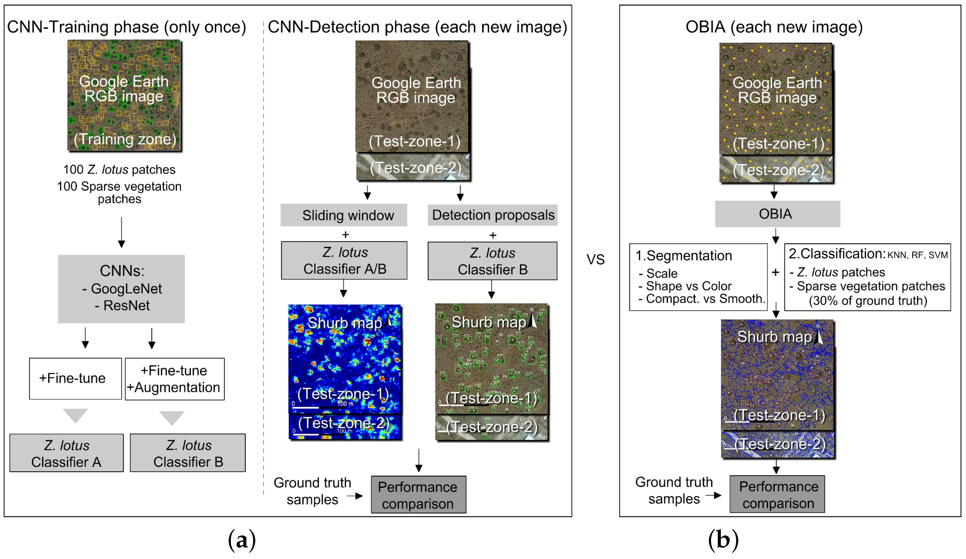
3. CNN-Based Detection for Shrub Mapping
3.1. Training Phase: CNN-Classifier With Fine-Tuning and Data Augmentation
- Transfer learning (e.g., fine-tuning in CNNs). The best analogy for transfer-learning could be the way humans face a new challenge. Humans do not start the learning from scratch, they always use previous knowledge to build new one. Transfer-learning consists of re-utilizing the knowledge learnt from one problem to another related one ([46]). Applying transfer learning with deep CNNs depends on the similarities between the original and new problem and also on the size of the new training set. In deep CNNs, transfer learning can be applied via fine-tuning, by initializing the weights of the network, in Equation (2), with the pre-trained weights from a different dataset.In general, fine-tuning the entire network (i.e., updating all the weights) is only used when the new dataset is large enough, otherwise, the model could suffer overfitting especially among the first layers of the network. Since these layers extract low-level features, e.g., edges and color, they do not change significantly and can be utilized for several visual recognition tasks. The last learnable layers of the CNN are gradually adjusted to the particularities of the problem and extract high level features.In this work, we have used fine-tuning on ResNet and GoogleNet. We initialized the used CNNs with the pre-trained weights of the same architectures on ImageNet dataset (around 1.28 million images over 1000 generic object classes) ([13]).
- Data-augmentation, also called data transformation or distortion, is used to artificially increase the number of samples in the training set by applying specific deformations on the input images, e.g., rotation, flipping, translation, cropping, or changing the brightness of the pixels. In this way, from a small number of initial samples, one can build a much larger dataset of transformed images that still are meaningful for the case study. The set of valid transformations that improves the performance of the CNN-model depends on the particularities of the problem. Several previous studies have demonstrated that increasing the size of the training dataset using different data-augmentation techniques increases performance and makes the learning of CNNs models robust to changes in scales, brightness and geometrical distortions [44,47].
3.2. Detection Phase
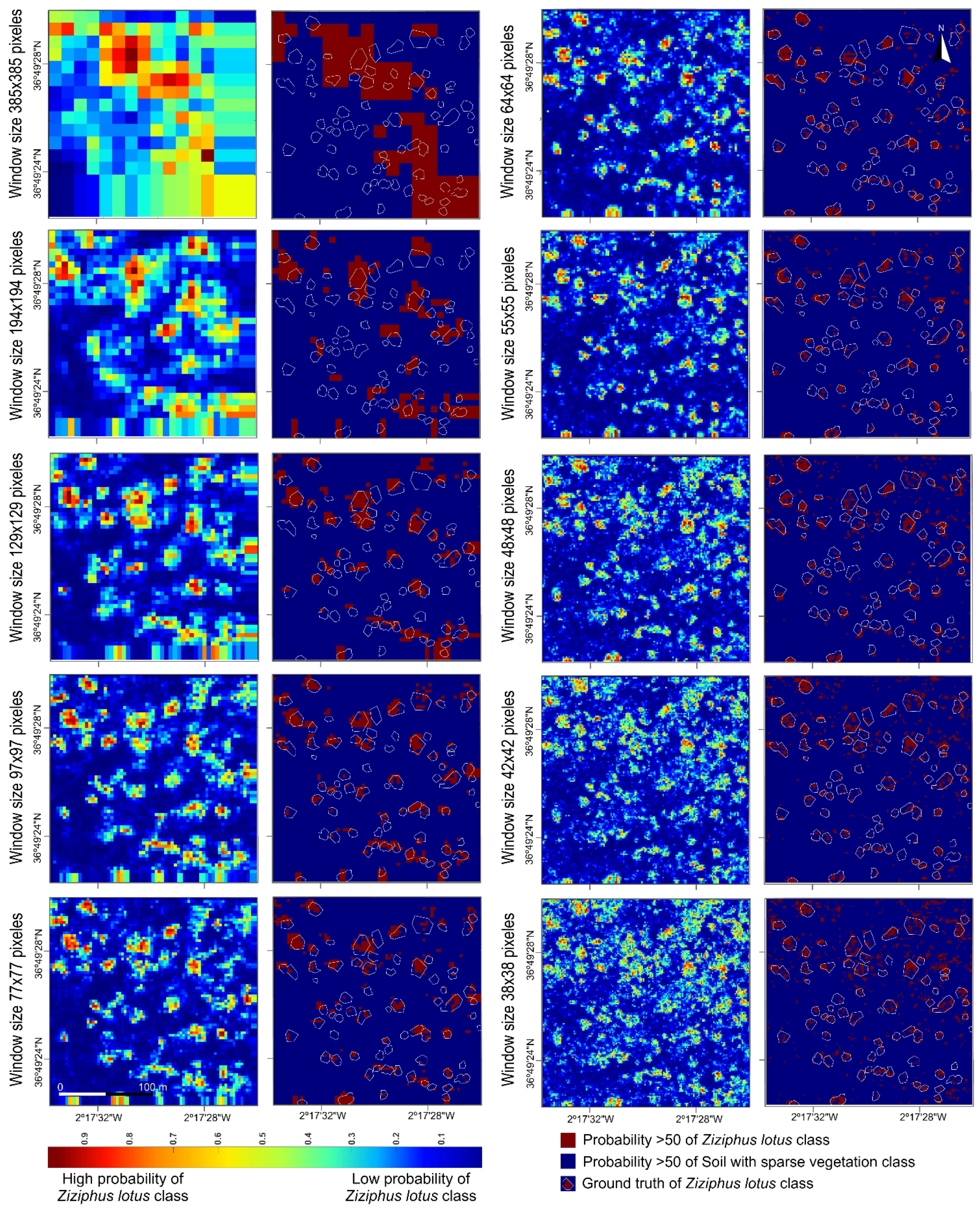
- Sliding window is an exhaustive technique frequently used for detection. It is based on the assumption that all the areas of the input-image are possible candidates to contain an object class. This search across the input-image can generate around candidate windows. The detection task consists of applying the obtained CNN-classifier at all locations and scales of the input image. The sliding window approach is an exhaustive method since it considers a very large number of candidate windows of different sizes and shapes across the input image. The classifier is then run on each one of these windows. To maximize the detection accuracy, the probabilities obtained from different window sizes can be assembled into one heatmap. Finally, probability heatmaps are usually transformed into classes using a thresholding technique, i.e., areas with probabilities higher than 50% are usually classified as the true class (e.g., Ziziphus lotus) and areas with probabilities lower than 50% as background (e.g., bare soil with sparse vegetation).
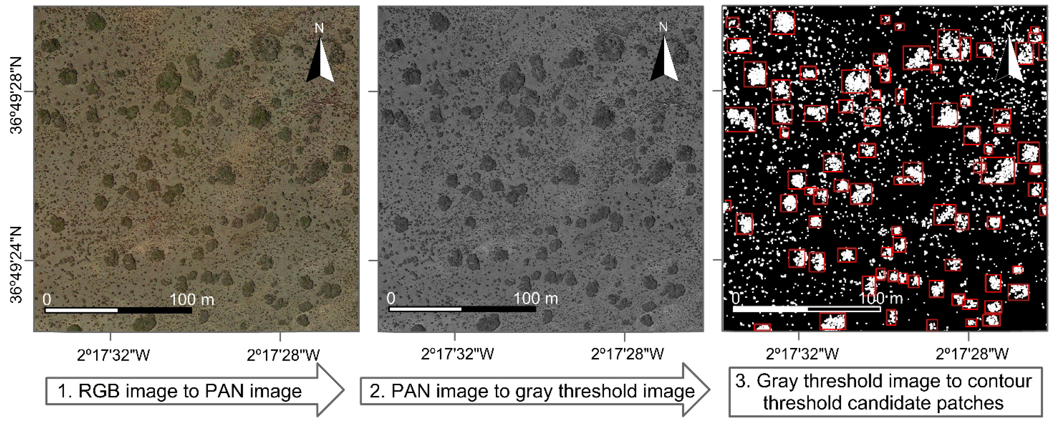
- Detection proposals are techniques that employ different selection criteria to reduce the number of candidate windows, thereby avoiding the exhaustive sliding window search ([48]). These techniques can also help to improve the detection accuracy and execution time. In general, detection proposals methods determine the set of pre-processing techniques that provides the best results. This set depends on the nature of the problem and the object of interest. From the multiple techniques that we explored, the ones that provided the best detection performance were: (i) Eliminating the background using a threshold based on its typical color or darkness (e.g., by converting the RGB image to gray scale, grays lighter than 100 digital level corresponded to bare ground). (ii) Applying an edge-detection method that filters out the objects with an area or perimeter smaller than the minimum size of the target objects (e.g., the area of the smallest Ziziphus lotus individual in the image, around 22 m).
4. Study Areas and Datasets Construction
4.1. Study Areas
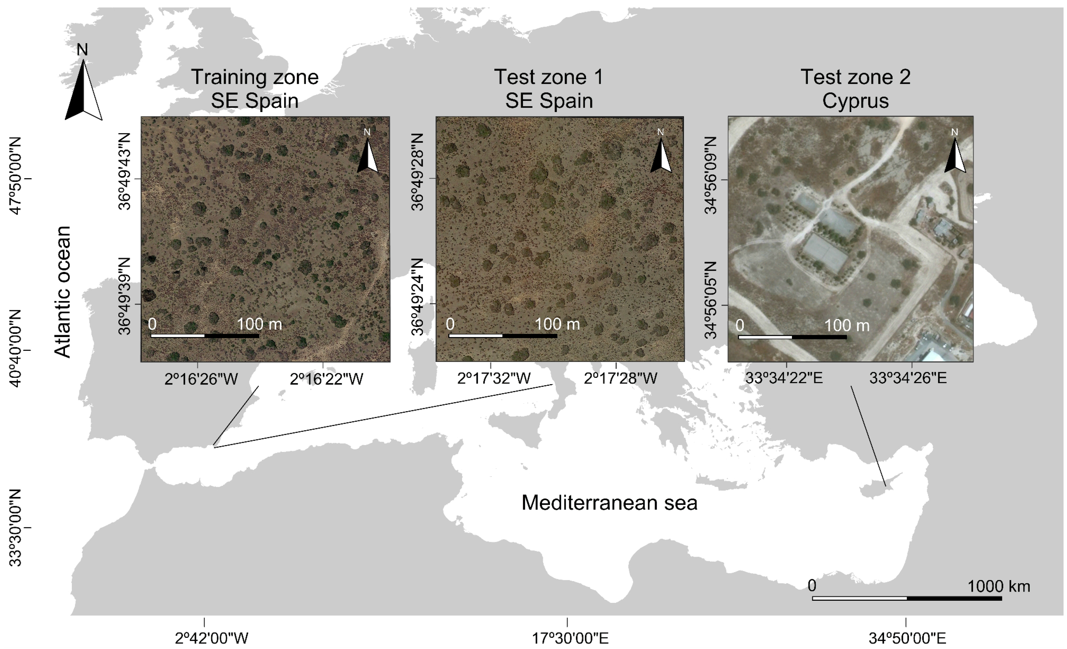
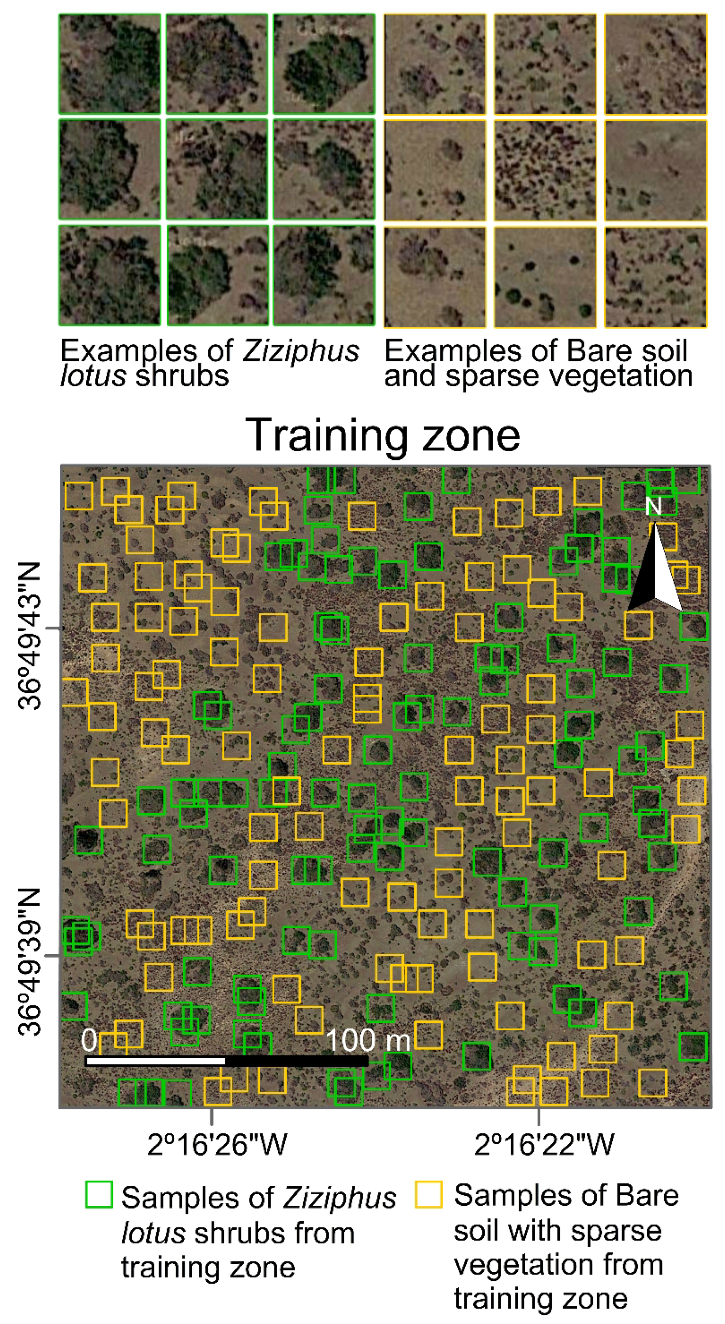
- The training-zone used for training the CNN-based model. This zone is located in Cabo de Gata-Níjar Natural Park, 364943 N, 21622 W, in the province of Almería, Spain (Figure 2). The climate is semi-arid Mediterranean. The vegetation is scarce and patchy, mainly dominated by large Ziziphus lotus shrubs surrounded by a heterogeneous matrix of bare soil and small scrubs (e.g., Thymus hyemalis, Launea arborescens and Lygeum spartum) with low coverage ([49,52]). Ziziphus lotus forms large hemispherical bushes with very deep roots and 1–3 m tall that trap and accumulate sand and organic matter building geomorphological structures, called nebkhas, that constitute a shelter micro-habitat for many plant and animal species ([19,49,53]).
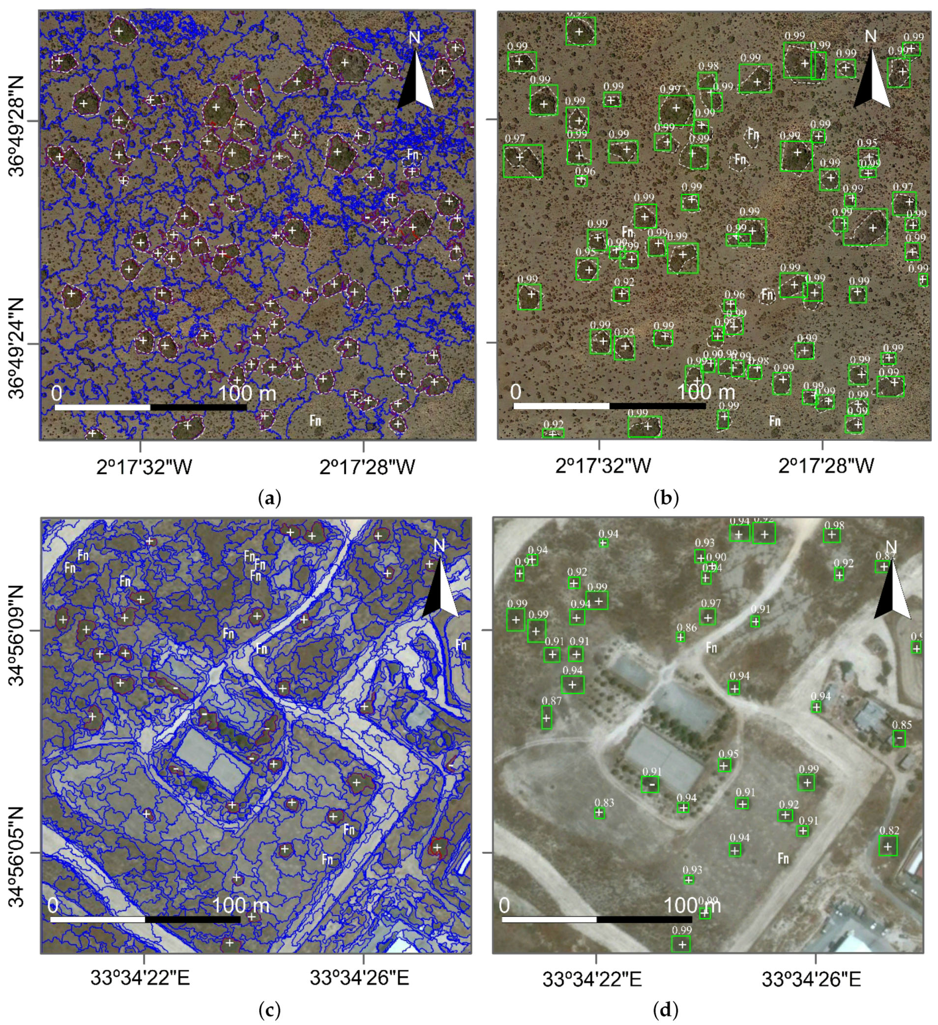
- Test-zone-1 and test-zone-2 belong to two different protected areas. Test-zone-1 is located km west from the training-zone, 364928 N, 21728 W. Test-zone-2 is located in Rizoelia National Forest Park in Cyprus, 345609 N, 333426 E (Figure 2). These two test-zones are used for comparing the performance between CNNs and OBIA for detecting Ziziphus lotus.
4.2. Datasets Construction
4.2.1. Satellite-Derived Orthoimages from Google Earth
- Training-zone and test-zone-1 images (SE Spain) were captured by Worldview-2 satellite under 0% cloud cover on the 30 June 2016, with an inclination angle of 12.7. The multispectral RGB bands have a native spatial resolution of 1.84 m, but they are pansharpened to 0.5 m by Worldview-2 using the panchromatic band. The RGB bands cover the following wavelength ranges: Red: 630–690 nm, Green: 510–580 nm, Blue: 450–510 nm.
- Test-zone-2 image (Cyprus) was captured by Pléiades-1A satellite under 0.1% cloud cover on the 8 July 2016, with an inclination angle of 29.2. The multi spectral RGB bands have a native spatial resolution of 2 m, but they are pansharpened to 0.5 m by Pléiades-1A using the panchromatic band. They RGB bands cover the following wavelength ranges: Red: 600–720 nm, Green: 490–610 nm, Blue: 430–550 nm.
4.2.2. Dataset for Training OBIA and for Ground Truthing
- In test-zone-1, 74 Ziziphus lotus individual were identified in the field. The perimeter of each was georeferenced in the field with a differential GPS, GS20, Leica Geosystems, Inc. From the 74 individual shrub, 30% (22 individual shrubs) were used for training and 70% (52 individuals) for validation in the OBIA method. Images containing patches from all 74 individual shrubs were used for validation in the CNN method (see below).
- In test-zone-2, 40 Ziziphus lotus individuals were visually identified in Google Earth by the authors using the vegetation maps and descriptions provided by local botany experts ([54]). These individuals were also validated in the field by one of the co-authors, J. Cabello. All 40 individual shrubs were used for validation in both the OBIA and CNN methods.In both test zones, the same number of Ziziphus lotus individuals (74 and 40, respectively) was georeferenced for the Bare soil with sparse vegetation class (Table 1).
4.2.3. Training Dataset for the CNN-Classifier
5. Experimental Evaluation and Discussions
5.1. Finding the Best CNN-Based Detector
5.1.1. CNN Training With Fine-Tuning and Data-Augumentation
- Random scale: increases the scale of the image by a factor picked randomly in [1 to 10%]
- Random crop: crops the image edges by a margin in [0 to 10%]
- Flip horizontally: randomly mirrors the image from left to right.
- Random brightness: multiplies the brightness of the image by a factor picked randomly in [0, 10].
5.1.2. Detection Using GoogLeNet Under the Sliding Window Approach
5.1.3. Detection Using GoogLeNet and ResNet under a Detection Proposals Approach
5.2. Finding the Best OBIA-Detector
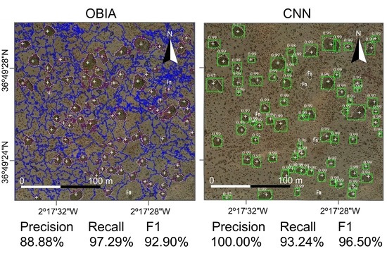
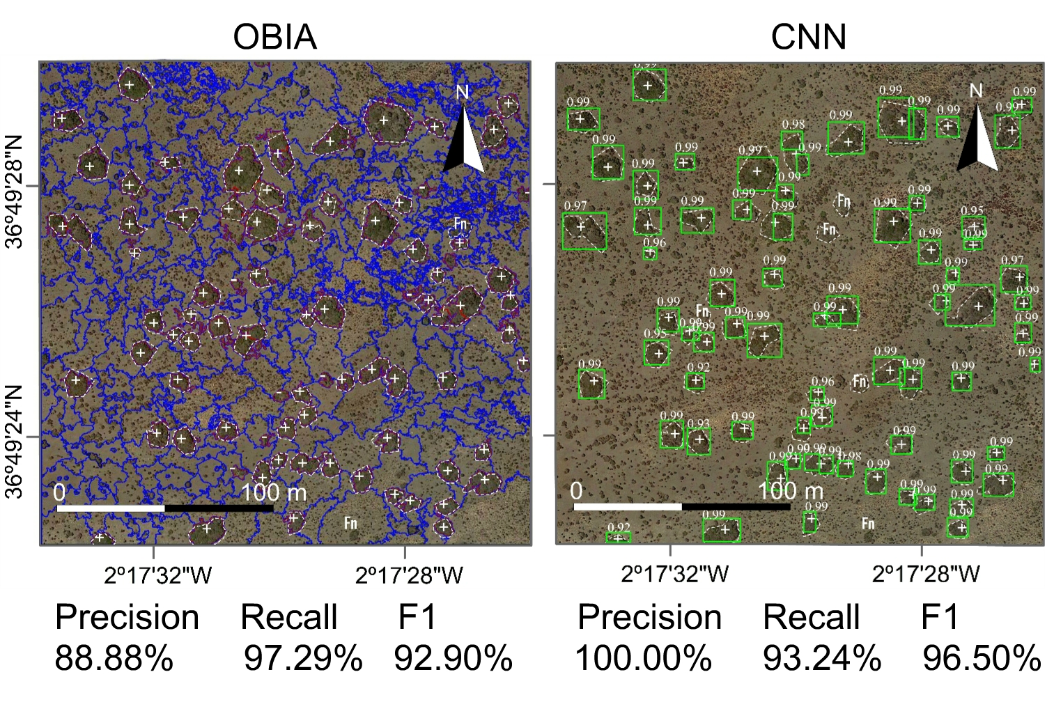
5.3. CNN-Detector Versus OBIA-Detector
6. Conclusions
Acknowledgments
Author Contributions
Conflicts of Interest
Abbreviations
| CNNs | Convolutional Neural Networks |
| OBIA | Object-Based Image Analysis |
References
- Congalton, R.; Gu, J.; Yadav, K.; Thenkabail, P.; Ozdogan, M. Global land cover mapping: A review and uncertainty analysis. Remote Sens. 2014, 6, 12070–12093. [Google Scholar] [CrossRef]
- Rogan, J.; Chen, D. Remote sensing technology for mapping and monitoring land-cover and land-use change. Prog. Plan. 2004, 61, 301–325. [Google Scholar] [CrossRef]
- Blaschke, T. Object based image analysis for remote sensing. ISPRS J. Photogramm. Remote Sens. 2010, 65, 2–16. [Google Scholar] [CrossRef]
- Li, X.; Shao, G. Object-based land-cover mapping with high resolution aerial photography at a county scale in midwestern USA. Remote Sens. 2014, 6, 11372–11390. [Google Scholar] [CrossRef]
- Pierce, K. Accuracy optimization for high resolution object-based change detection: An example mapping regional urbanization with 1-m aerial imagery. Remote Sens. 2015, 7, 12654–12679. [Google Scholar] [CrossRef]
- Ecognition. Available online: http://www.ecognition.com (accessed on 5 May 2017).
- Knoth, C.; Nüst, D. Reproducibility and Practical Adoption of GEOBIA with Open-Source Software in Docker Containers. Remote Sens. 2017, 9, 290. [Google Scholar] [CrossRef]
- Teodoro, A.; Araújo, R. Exploration of the OBIA methods available in SPRING noncommercial software to UAV data processing. In Proceedings of the Earth Resources and Environmental Remote Sensing/GIS Applications V, Amsterdam, The Netherlands, 10 October 2014; Volume 9245. [Google Scholar]
- Pal, M. Random forest classifier for remote sensing classification. Int. J. Remote Sens. 2005, 26, 217–222. [Google Scholar] [CrossRef]
- Heumann, B.W. An object-based classification of mangroves using a hybrid decision tree—Support vector machine approach. Remote Sens. 2011, 3, 2440–2460. [Google Scholar] [CrossRef]
- Feng, Q.; Liu, J.; Gong, J. UAV remote sensing for urban vegetation mapping using random forest and texture analysis. Remote Sens. 2015, 7, 1074–1094. [Google Scholar] [CrossRef]
- Ma, L.; Li, M.; Ma, X.; Cheng, L.; Du, P.; Liu, Y. A review of supervised object-based land-cover image classification. ISPRS J. Photogramm. Remote Sens. 2017, 130, 277–293. [Google Scholar] [CrossRef]
- Krizhevsky, A.; Sutskever, I.; Hinton, G.E. ImageNet Classification with Deep Convolutional Neural Networks. In Proceedings of the 25th International Conference on Neural Information Processing Systems, Lake Tahoe, NV, USA, 3–6 December 2012; Curran Associates Inc.: Red Hook, NY, USA, 2012; Volume 1, pp. 1097–1105. [Google Scholar]
- Le, Q.V. Building high-level features using large scale unsupervised learning. In Proceedings of the 2013 IEEE International Conference on Acoustics, Speech and Signal Processing, Vancouver, BC, Canada, 26–31 May 2013; pp. 8595–8598. [Google Scholar]
- Hinton, G.; Deng, L.; Yu, D.; Dahl, G.; Mohamed, A.; Jaitly, N.; Senior, A.; Vanhoucke, V.; Nguyen, P.; Sainath, T.; et al. Deep Neural Networks for Acoustic Modeling in Speech Recognition: The Shared Views of Four Research Groups. IEEE Signal Process. Mag. 2012, 29, 82–97. [Google Scholar] [CrossRef]
- Sainath, T.N.; Mohamed, A.; Kingsbury, B.; Ramabhadran, B. Deep convolutional neural networks for LVCSR. In Proceedings of the 2013 IEEE International Conference on Acoustics, Speech and Signal Processing, Vancouver, BC, Canada, 26–31 May 2013; pp. 8614–8618. [Google Scholar]
- Zhu, X.X.; Tuia, D.; Mou, L.; Xia, G.S.; Zhang, L.; Xu, F.; Fraundorfer, F. Deep learning in remote sensing: A review. arXiv Prepr. 2017; arXiv:1710.03959. [Google Scholar]
- Abadi, M.; Agarwal, A.; Barham, P.; Brevdo, E.; Chen, Z.; Citro, C.; Corrado, G.; Davis, A.; Dean, J.; Devin, M.; et al. Tensorflow: Large-scale machine learning on heterogeneous distributed systems. arXiv Prepr. 2016; arXiv:1603.04467. [Google Scholar]
- Tirado, R. 5220 Matorrales arborescentes con Ziziphus (*). In VV. AA., Bases ecológicas Preliminares Para la Conservación de Los Tipos de Hábitat de Interés Comunitario en Espana; Ministerio de Medio Ambiente, Medio Rural y Marino: Madrid, Spain, 2009. [Google Scholar]
- Zhao, W.; Du, S.; Emery, W. Object-Based Convolutional Neural Network for High-Resolution Imagery Classification. IEEE J. Sel. Top. Appl. Earth Observ. Remote Sens. 2017, 10, 3386–3396. [Google Scholar] [CrossRef]
- Längkvist, M.; Kiselev, A.; Alirezaie, M.; Loutfi, A. Classification and segmentation of satellite orthoimagery using convolutional neural networks. Remote Sens. 2016, 8, 329. [Google Scholar] [CrossRef]
- Hu, F.; Xia, G.; Hu, J.; Zhang, L. Transferring deep convolutional neural networks for the scene classification of high-resolution remote sensing imagery. Remote Sens. 2015, 7, 14680–14707. [Google Scholar] [CrossRef]
- Santara, A.; Mani, K.; Hatwar, P.; Singh, A.; Garg, A.; Padia, K.; Mitra, P. BASS Net: Band-Adaptive Spectral-Spatial Feature Learning Neural Network for Hyperspectral Image Classification. arXiv Prepr. 2016; arXiv:1612.00144. [Google Scholar]
- Ding, C.; Li, Y.; Xia, Y.; Wei, W.; Zhang, L.; Zhang, Y. Convolutional Neural Networks Based Hyperspectral Image Classification Method with Adaptive Kernels. Remote Sens. 2017, 9, 618. [Google Scholar] [CrossRef]
- Liang, H.; Li, Q. Hyperspectral imagery classification using sparse representations of convolutional neural network features. Remote Sens. 2016, 8, 99. [Google Scholar] [CrossRef]
- Hyperspectral Remote Sensing Scenes. Available online: http://www.ehu.eus/ccwintco/index.php?title=Hyperspectral_Remote_Sensing_Scenes (accessed on 25 November 2017).
- UC Merced Land Use Dataset. Available online: http://weegee.vision.ucmerced.edu/datasets/landuse.html (accessed on 25 November 2017).
- Brazilian Coffee Scenes Dataset. Available online: http://www.patreo.dcc.ufmg.br/2017/11/12/brazilian-coffee-scenes-dataset/ (accessed on 25 November 2017).
- Castelluccio, M.; Poggi, G.; Sansone, C.; Verdoliva, L. Land use classification in remote sensing images by convolutional neural networks. arXiv Prepr. 2015; arXiv:1508.00092. [Google Scholar]
- Li, W.; Fu, H.; Yu, L.; Cracknell, A. Deep Learning Based Oil Palm Tree Detection and Counting for High-Resolution Remote Sensing Images. Remote Sens. 2016, 9, 22. [Google Scholar] [CrossRef]
- Tiede, D.; Krafft, P.; Füreder, P.; Lang, S. Stratified Template Matching to Support Refugee Camp Analysis in OBIA Workflows. Remote Sens. 2017, 9, 326. [Google Scholar] [CrossRef]
- Laliberte, A.S.; Rango, A.; Havstad, K.M.; Paris, J.F.; Beck, R.F.; McNeely, R.; Gonzalez, A.L. Object-oriented image analysis for mapping shrub encroachment from 1937 to 2003 in southern New Mexico. Remote Sens. Environ. 2004, 93, 198–210. [Google Scholar] [CrossRef]
- Hellesen, T.; Matikainen, L. An object-based approach for mapping shrub and tree cover on grassland habitats by use of LiDAR and CIR orthoimages. Remote Sens. 2013, 5, 558–583. [Google Scholar] [CrossRef]
- Stow, D.; Hamada, Y.; Coulter, L.; Anguelova, Z. Monitoring shrubland habitat changes through object-based change identification with airborne multispectral imagery. Remote Sens. Environ. 2008, 112, 1051–1061. [Google Scholar] [CrossRef]
- Baatz, M.; Schäpe, A. Multiresolution segmentation: An optimization approach for high quality multi-scale image segmentation. Angew. Geogr. Inf. XII 2000, 58, 12–23. [Google Scholar]
- Tian, J.; Chen, D.M. Optimization in multi-scale segmentation of high-resolution satellite images for artificial feature recognition. Int. J. Remote Sens. 2007, 28, 4625–4644. [Google Scholar] [CrossRef]
- Liu, Y.; Bian, L.; Meng, Y.; Wang, H.; Zhang, S.; Yang, Y.; Shao, X.; Wang, B. Discrepancy measures for selecting optimal combination of parameter values in object-based image analysis. ISPRS J. Photogramm. Remote Sens. 2012, 68, 144–156. [Google Scholar] [CrossRef]
- Belgiu, M.; Drăguţ, L. Random forest in remote sensing: A review of applications and future directions. ISPRS J. Photogramm. Remote Sens. 2016, 114, 24–31. [Google Scholar] [CrossRef]
- Ghosh, A.; Joshi, P. A comparison of selected classification algorithms for mapping bamboo patches in lower Gangetic plains using very high resolution WorldView 2 imagery. Int. J. Appl. Earth Observ. Geoinf. 2014, 26, 298–311. [Google Scholar] [CrossRef]
- Congalton, R.; Green, K. Assessing the Accuracy of Remotely Sensed Data: Principles and Practices; CRC Press: Boca Raton, FL, USA, 2008. [Google Scholar]
- Guo, Y.; Liu, Y.; Oerlemans, A.; Lao, S.; Wu, S.; Lew, M. Deep learning for visual understanding: A review. Neurocomputing 2016, 187, 27–48. [Google Scholar] [CrossRef]
- He, K.; Zhang, X.; Ren, S.; Sun, J. Deep residual learning for image recognition. In Proceedings of the IEEE Conference on Computer Vision and Pattern Recognition, Las Vegas, NV, USA, 27–30 June 2016; pp. 770–778. [Google Scholar]
- Szegedy, C.; Liu, W.; Jia, Y.; Sermanet, P.; Reed, S.; Anguelov, D.; Erhan, D.; Vanhoucke, V.; Rabinovich, A. Going deeper with convolutions. In Proceedings of the IEEE Conference on Computer Vision and Pattern Recognition, Boston, MA, USA, 7–12 June 2015; pp. 1–9. [Google Scholar]
- Tabik, S.; Peralta, D.; Herrera-Poyatos, A.; Herrera, F. A snapshot of image pre-processing for convolutional neural networks: Case study of MNIST. Int. J. Comput. Intell. Syst. 2017, 10, 555–568. [Google Scholar] [CrossRef]
- Shin, H.; Roth, H.R.; Gao, M.; Lu, L.; Xu, Z.; Nogues, I.; Yao, J.; Mollura, D.; Summers, R.M. Deep convolutional neural networks for computer-aided detection: CNN architectures, dataset characteristics and transfer learning. IEEE Trans. Med. Imaging 2016, 35, 1285–1298. [Google Scholar] [CrossRef] [PubMed]
- Pan, S.J.; Yang, Q. A survey on transfer learning. IEEE Trans. Knowl. Data Eng. 2010, 22, 1345–1359. [Google Scholar] [CrossRef]
- Peralta, D.; Triguero, I.; Garcia, S.; Saeys, Y.; Benitez, J.; Herrera, F. On the use of convolutional neural networks for robust classification of multiple fingerprint captures. Int. J. Intell. Syst. 2018, 33, 213–230. [Google Scholar] [CrossRef]
- Hosang, J.; Benenson, R.; Dollar, P.; Schiele, B. What makes for effective detection proposals. IEEE Trans. Pattern Anal. Mach. Intell. 2016, 38, 814–830. [Google Scholar] [CrossRef] [PubMed]
- Tirado, R.; Pugnaire, F. Shrub spatial aggregation and consequences for reproductive success. Oecologia 2003, 136, 296–301. [Google Scholar] [CrossRef] [PubMed]
- Guirado, E. Factores que Afectan a la Distribucion Especial de Vegetacion Freatofita (Zipiphus lotus) en el Acuifero Costero de Torre Garcia (Sureste de España). Master Thesis, University of Almería, Almería, Spain, 2015. [Google Scholar]
- Guirado, E.; Alcaraz-Segura, D.; Rigol-Sanchez, J.; Gisbert, J.; Martinez-Moreno, F.; Galindo-Zaldivar, J.; Gonzalez-Castillo, L.; Cabello, J. Remote sensing-derived fractures and shrub patterns to identify groundwater dependence. Ecohydrology 2017. accepted. [Google Scholar]
- Rivas Goday, S.; Bellot, F. Las formaciones de Zizyphus lotus (L.) Lamk., en las dunas del Cabo de Gata. Anales del Instituto Español de Edafología, Ecología y Fisiología Vegetal 1944, 3, 109–126. [Google Scholar]
- Lagarde, F.; Louzizi, T.; Slimani, T.; El Mouden, H.; Kaddour, K.; Moulherat, S.; Bonnet, X. Bushes protect tortoises from lethal overheating in arid areas of Morocco. Environ. Conserv. 2012, 39, 172–182. [Google Scholar] [CrossRef]
- Manolaki, P.; Andreou, M.; Christodoulou, C. Improving the conservation status of priority habitat types 1520 and 5220 at Rizoelia National Forest Park. EC LIFE Project. Available online: http://www.life-rizoelia.eu (accessed on 25 October 2017).
- Nussbaum, S.; Niemeyer, I.; Canty, M. SEATH—A New Tool for Automated Feature Extraction in the Context of Object-Based Image Analysis; 1st International Conference; Object-Based Image Analysis (OBIA): Salzburg, Austria, 2006. [Google Scholar]
- García García, J.; Sánchez Caparrós, A.; Castillo, E.; Marín, I.; Padilla, A.; Rosso, J. Hidrogeoquímica de las aguas subterráneas en la zona de Cabo de Gata. In López-Geta JA, Gómez JD, De la Orden JA, Ramos G. and Rodríguez L. Tecnología de la Intrusión de Agua de mar en Acuíferos Costeros: Países Mediterráneos; IGME: Madrid, Spain, 2003; pp. 413–422. [Google Scholar]
- Poli, D.; Remondino, F.; Angiuli, E.; Agugiaro, G. Radiometric and geometric evaluation of GeoEye-1, WorldView-2 and Pléiades-1A stereo images for 3D information extraction. ISPRS J. Photogramm. Remote Sens. 2015, 100, 35–47. [Google Scholar] [CrossRef]
- Basaeed, E.; Bhaskar, H.; Al-Mualla, M. CNN-based multi-band fused boundary detection for remotely sensed images. In Proceedings of the 6th International Conference on Imaging for Crime Prevention and Detection (ICDP-15), IET, London, UK, 15–17 July 2015; p. 11. [Google Scholar]
- Drăguţ, L.; Csillik, O.; Eisank, C.; Tiede, D. Automated parameterisation for multi-scale image segmentation on multiple layers. ISPRS J. Photogramm. Remote Sens. 2014, 88, 119–127. [Google Scholar] [CrossRef] [PubMed]
- Bastin, J.; Berrahmouni, N.; Grainger, A.; Maniatis, D.; Mollicone, D.; Moore, R.; Patriarca, C.; Picard, N.; Sparrow, B.; Abraham, E.; et al. The extent of forest in dryland biomes. Science 2017, 356, 635–638. [Google Scholar] [CrossRef] [PubMed]
- Schepaschenko, D.; Fritz, S.; See, L.; Bayas, J.C.L.; Lesiv, M.; Kraxner, F.; Obersteiner, M. Comment on “The extent of forest in dryland biomes”. Science 2017, 358, eaao0166. [Google Scholar] [CrossRef] [PubMed]
- Prevedello, J.A.; Almeida-Gomes, M.; Lindenmayer, D. The importance of scattered trees for biodiversity conservation: A global meta-analysis. J. Appl. Ecol. 2017, in press. [Google Scholar] [CrossRef]
- Griffith, D.M.; Lehmann, C.E.; Strömberg, C.A.; Parr, C.L.; Pennington, R.T.; Sankaran, M.; Ratnam, J.; Still, C.J.; Powell, R.L.; Hanan, N.P.; et al. Comment on “The extent of forest in dryland biomes”. Science 2017, 358, eaao1309. [Google Scholar] [CrossRef] [PubMed]
- de la Cruz, M.; Quintana-Ascencio, P.F.; Cayuela, L.; Espinosa, C.I.; Escudero, A. Comment on “The extent of forest in dryland biomes”. Science 2017, 358, eaao0369. [Google Scholar] [CrossRef] [PubMed]
- Pettorelli, N.; Wegmann, M.; Skidmore, A.; Mücher, S.; Dawson, T.P.; Fernandez, M.; Lucas, R.; Schaepman, M.E.; Wang, T.; O’Connor, B.; et al. Framing the concept of satellite remote sensing essential biodiversity variables: challenges and future directions. Remote Sens. Ecol. Conserv. 2016, 2, 122–131. [Google Scholar] [CrossRef]


| CNN Classifier | OBIA Classifier | Accuracy | ||||
|---|---|---|---|---|---|---|
| Class | Training | Validation | Training | Assessment | ||
| Training-Zone | Test-Zone-1 | Test-Zone-2 | Test-Zone-1 | Test-Zone-2 | ||
| Ziziphus | 80 img | 20 img | 22 poly | 0 poly | 52 poly | 40 poly |
| Bare soil | 80 img | 20 img | 22 poly | 0 poly | 2 poly | 40 poly |
| Detection Model | TP | FP | FN | Precision | Recall | F1 |
|---|---|---|---|---|---|---|
| GoogLeNet (test-zone-1) +fine-tuning under sliding window | 65 | 12 | 9 | 77.64% | 89.18% | 83.01% |
| GoogLeNet (test-zone-1) +fine-tuning +augmentation under sliding window | 65 | 7 | 9 | 90.28% | 87.83% | 89.04% |
| GoogLeNet (test-zone-1) +fine-tuning +augmentation under detection proposals | 69 | 1 | 5 | 98.57% | 93.24% | 95.83% |
| ResNet (test-zone-1) +fine-tuning +augmentation under detection proposals | 69 | 0 | 5 | 100.00% | 93.24% | 96.50% |
| Win. Size (Pixels) | Total # of Win. | TP | FP | FN | Precis. (%) | Recall (%) | F1-Meas. (%) | Time (min) |
|---|---|---|---|---|---|---|---|---|
| 385×385 | 196 | 31 | 18 | 41 | 63.27 | 43.06 | 51.24 | 6.0 |
| 194×194 | 961 | 34 | 7 | 38 | 82.93 | 47.22 | 60.18 | 29.4 |
| 129×129 | 2209 | 42 | 6 | 30 | 87.50 | 58.33 | 70.00 | 67.6 |
| 97× 97 | 4096 | 59 | 6 | 13 | 90.77 | 81.94 | 86.13 | 125.4 |
| 77×77 | 5929 | 59 | 5 | 13 | 92.19 | 81.94 | 86.76 | 181.5 |
| 64×64 | 9506 | 65 | 7 | 7 | 90.28 | 90.28 | 90.28 | 291.0 |
| 55×55 | 13,340 | 65 | 12 | 7 | 84.42 | 90.28 | 87.25 | 408.4 |
| 48×48 | 17,292 | 68 | 16 | 4 | 80.95 | 94.44 | 87.18 | 529.3 |
| 42×42 | 22,200 | 70 | 17 | 2 | 80.46 | 97.22 | 88.05 | 679.6 |
| 38× 38 | 27,888 | 71 | 39 | 1 | 64.55 | 98.61 | 78.02 | 853.7 |
| Detection Model | TP | FP | FN | Precision | Recall | F1 |
|---|---|---|---|---|---|---|
| >ResNet-based classifier (test-zone-1) +fine-tuning +augmentation under detection proposals | 69 | 0 | 5 | 100.00% | 93.24% | 96.50% |
| OBIA-KNN (test-zone-1) | 66 | 9 | 8 | 88.00% | 89.18% | 88.59% |
| OBIA-Random Forest (test-zone-1) | 67 | 6 | 7 | 91.78% | 90.54% | 91.15 % |
| OBIA-SVM (test-zone-1) | 72 | 9 | 2 | 88.88% | 97.29% | 92.90% |
| >ResNet-based classifier (test-zone-2) +fine-tuning +augmentation under detection proposals | 38 | 3 | 2 | 92.68% | 95.00% | 93.38% |
| OBIA-KNN (test-zone-2) | 21 | 4 | 19 | 84.00% | 52.50% | 64.61% |
| OBIA-Random Forest (test-zone-2) | 27 | 6 | 13 | 81.81% | 67.5% | 73.97% |
| OBIA-SVM (test-zone-2) | 29 | 6 | 11 | 82.85% | 72.50% | 77.33% |
© 2017 by the authors. Licensee MDPI, Basel, Switzerland. This article is an open access article distributed under the terms and conditions of the Creative Commons Attribution (CC BY) license (http://creativecommons.org/licenses/by/4.0/).
Share and Cite
Guirado, E.; Tabik, S.; Alcaraz-Segura, D.; Cabello, J.; Herrera, F. Deep-learning Versus OBIA for Scattered Shrub Detection with Google Earth Imagery: Ziziphus lotus as Case Study. Remote Sens. 2017, 9, 1220. https://doi.org/10.3390/rs9121220
Guirado E, Tabik S, Alcaraz-Segura D, Cabello J, Herrera F. Deep-learning Versus OBIA for Scattered Shrub Detection with Google Earth Imagery: Ziziphus lotus as Case Study. Remote Sensing. 2017; 9(12):1220. https://doi.org/10.3390/rs9121220
Chicago/Turabian StyleGuirado, Emilio, Siham Tabik, Domingo Alcaraz-Segura, Javier Cabello, and Francisco Herrera. 2017. "Deep-learning Versus OBIA for Scattered Shrub Detection with Google Earth Imagery: Ziziphus lotus as Case Study" Remote Sensing 9, no. 12: 1220. https://doi.org/10.3390/rs9121220
APA StyleGuirado, E., Tabik, S., Alcaraz-Segura, D., Cabello, J., & Herrera, F. (2017). Deep-learning Versus OBIA for Scattered Shrub Detection with Google Earth Imagery: Ziziphus lotus as Case Study. Remote Sensing, 9(12), 1220. https://doi.org/10.3390/rs9121220