Combining Estimation of Green Vegetation Fraction in an Arid Region from Landsat 7 ETM+ Data

Abstract

Fractional vegetation cover (FVC), or green vegetation fraction, is an important parameter for characterizing conditions of the land surface vegetation, and also a key variable of models for simulating cycles of water, carbon and energy on the land surface. There are several types of FVC estimation models using remote sensing data, and evaluating their performance over a specific region is of great significance. Therefore, this study firstly evaluated three types of FVC estimation models using Landsat 7 ETM+ data in an agriculture region of Heihe River Basin, China, and then proposed a combination strategy from different individual models to improve the FVC estimation accuracy, which employed the multiple linear regression (MLR) and Bayesian model average (BMA) methods. The validation results indicated that the spectral mixture analysis model with three endmembers (SMA3) achieved the best FVC estimation accuracy (determination coefficient (R²) = 0.902, root mean square error (RMSE) = 0.076) among the seven individual models using Landsat 7 ETM+ data. In addition, the MLR and BMA combination methods could both improve FVC estimation accuracy (R² = 0.913, RMSE = 0.063 and R² = 0.904, RMSE = 0.069 for MLR and BMA, respectively). Therefore, it could be concluded that both MLR and BMA combination methods integrating FVC estimates from different models using Landsat 7 ETM+ data could effectively weaken the estimation errors of individual models and improve the final FVC estimation accuracy.

1. Introduction

Fractional vegetation cover (FVC), or green vegetation fraction, is usually defined as the fraction of green vegetation as seen from the nadir of the total statistical area [1,2,3,4]. FVC is an important parameter for describing conditions of land surface vegetation, and a key indicator for monitoring the changes in ecosystems. Furthermore, these vegetation conditions and changes are important factors of specific models such as numerical weather prediction, regional and global climate modeling, and global change studies [5,6,7,8,9,10]. FVC has also been widely used for crop yield estimation, crop condition monitoring, drought monitoring and so on [11,12,13,14,15,16,17]. Therefore, it is of great significance to accurately estimate FVC on the regional and global scales.

To estimate the FVC in a large area, remote sensing technology has been the effective means, and several types of FVC estimation methods have been developed using remote sensing data, such as the regression models, the pixel dimidiate model, the three gradient differential vegetation index (TGDVI) model, the spectral mixture analysis (SMA), neural networks, and physical models. A regression model is an empirical FVC estimation method which establishes linear or non-linear relationships between FVC and vegetation indices (VIs) [18,19,20] or reflectances of various spectral bands [21]. The FVC estimation accuracy of a regression model is acceptable on a small regional scale using sufficient ground FVC measurements. However, the regression model cannot be extended to large scale FVC estimation because a single empirical model is usually generated for a specific vegetation type in the specific region, and the quantitative empirical relationship between FVC and vegetation indices or bands’ reflectance varies with vegetation types and regions. Thus, if the regression model is used for large regions, a large amount of ground measurements, covering various vegetation types and growth conditions, are required for accurately parameterizing the empirical models. This translates to a large quantity of work.

The pixel dimidiate model is a simple and widely used method for FVC estimation using remote sensing data, which assumes that one pixel is only composed of either vegetation or non-vegetation, and the fraction of vegetation composition is considered to be the FVC of this pixel [22,23,24,25,26]. Usually, a vegetation index is used as an indicator in the pixel dimidiate model, and the key issue of the pixel dimidiate model is determining the values of the vegetation index for pure vegetation and pure soil pixels. The pixel dimidiate model is simple and can achieve acceptable FVC estimation accuracy in small regions, but the determination of the parameters of the pixel dimidiate model is difficult because they vary with vegetation types and growth conditions.

The TGDVI model was developed based on the characteristics of vegetation and soil spectral reflectance, in which the maximal gradient difference is calculated using the green, red and near-infrared (NIR) bands’ reflectances [27]. Furthermore, Jiapaer et al. found that there were significant differences between vegetation and non-vegetation in short-wave infrared (SWIR), red and NIR bands [27]. Thus, the authors proposed two modified TGDVI (MTGDVI) models using Landsat 5 TM data to obtain more accurate FVC estimates in arid regions. The TGDVI model for FVC estimation is also simple and it also presents difficulties in determining the model parameters of the pure vegetation pixel because it also varies with vegetation types and growth conditions.

The SMA model can estimate the FVC from multi-spectral and hyper-spectral remote sensing data with the assumption that the spectral reflectance of one pixel is contributed to by all of the endmembers in the pixel. This model estimates FVC by calculating the fraction of vegetation endmembers [27,28,29,30,31,32]. The linear SMA model assumes that the reflectances of different endmembers are composed in a linear form in the mixture pixel which is commonly used for FVC estimation using remote sensing data. A similar assumption is made for the nonlinear SMA model, in which the reflectance of different endmembers are composed in a non-linear form [28,30,33,34]. The number and purity of the endmembers can obviously influence the accuracy of FVC estimates using SMA, thus a substantial difficulty in the SMA model is how to determine the endmembers and the spectral response of endmembers, because the land surface is very complex, especially for the development of a large scale SMA model.

Physical methods are usually based on the inversion of radiative transfer models which simulate the physical relationships between vegetation canopy spectral reflectance and FVC. However, due to the difficulties of the direct inversion of radiative transfer models [2], neural networks (NNs) and lookup table methods are usually employed for simplifying the inversion of physical models. NNs have been trained with physical model simulations and used to estimate FVC from several low spatial resolution sensors on large scale, such as in the POLDER FVC product and the CYCLOPES FVC product [8,35]. The physical methods are more widely acceptable in a theoretical sense. However, use of physical methods may be restricted due to the lack of suitable data because large amounts of data are required and many factors such as time, space, angle and spectral response need to be considered in the application of satellite remote sensing data.

Different FVC estimation models may have variational performance in different regions. Hence, evaluating the performance of different models is an important issue. This study mainly focuses on comparing the performances of different FVC estimation methods using Landsat 7 ETM+ data in an arid region and proposing two combination strategies, including multiple linear regression (MLR) and Bayesian model averaging (BMA) methods, to improve FVC estimation accuracy. Firstly, seven individual FVC estimation models, including the pixel dimidiate models with normalized difference vegetation index (NDVI) and enhanced vegetation index (EVI) as indicators, the SMA models using three and four endmembers, and three TGDVI models, were investigated using Landsat 7 ETM+ data. Then, the FVC estimates from individual models were combined in different ways using the MLR and BMA methods to improve FVC estimation accuracy. Finally, the performance of the individual models and the two combination methods were evaluated based on the ground FVC measurements.

2. Materials and Methods

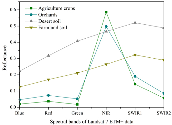
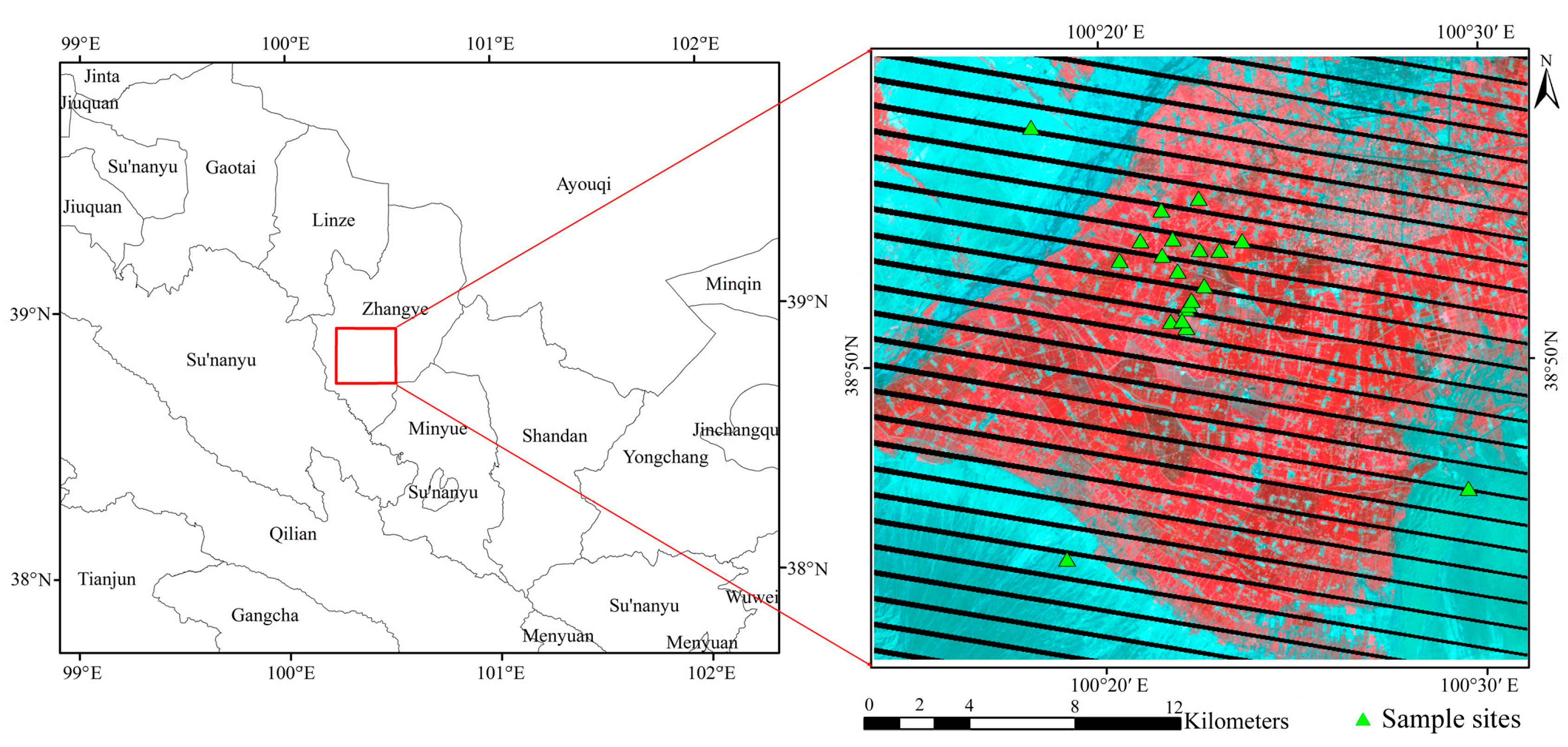
2.1. Study Area

The Heihe River basin (HRB) in the arid region of Northwest China was selected for this study (Figure 1). The HRB is the second largest inland river basin in China, which is also the experimental area for the HiWATER project [36]. The study area is located around the oasis, which is located in the middle of the HRB (38°50′7″N, 100°22′34″E), and covers approximately 570 km². The annual precipitation is approximately 100–250 mm and the annual mean temperature is approximately 7–10 °C. The land surface is mainly occupied by agriculture crops, mostly corn. The growing season of corn is from May to September. Small patches of orchards, vegetables and wheat are also found in the agriculture region. The Gobi Desert is located around the oasis and some desert vegetation is found in this region, such as camel thorn.

2.2. Landsat 7 ETM+ Data

Three Landsat 7 ETM+ data, in path 133 and row 33, with cloud coverage of less than 10% in 2012 were selected for this study. The dates that these Landsat 7 ETM+ data sets were obtained were the closest possible to the dates of the field FVC measurements (

Table 1. Dates of the Landsat 7 ETM+ data acquisition, field FVC measurements, and number of valid field FVC measurements.

	Day 1	Day 2	Day 3
Landsat 7 ETM+	24 June 2012	12 July 2012	28 August 2012
Field survey data	23 June 2012	10 July 2012	28 August 2012
Number of valid field data	15	19	10

). The exact dates of acquisition of the three Landsat ETM+ data sets were 24 June, 12 July and 28 August 2012. The Landsat 7 ETM+ data were downloaded from the United States Geological Survey (USGS) website (http://earthexplorer.usgs.gov/). They had already been processed with atmospheric and geometric corrections. The atmospheric correction of the Landsat 7 ETM+ data was completed using the Landsat Ecosystem Disturbance Adaptive Processing System (LEDAPS) software, and the top of canopy reflectances of Landsat 7 ETM+ data were used for FVC estimation in the further analysis.

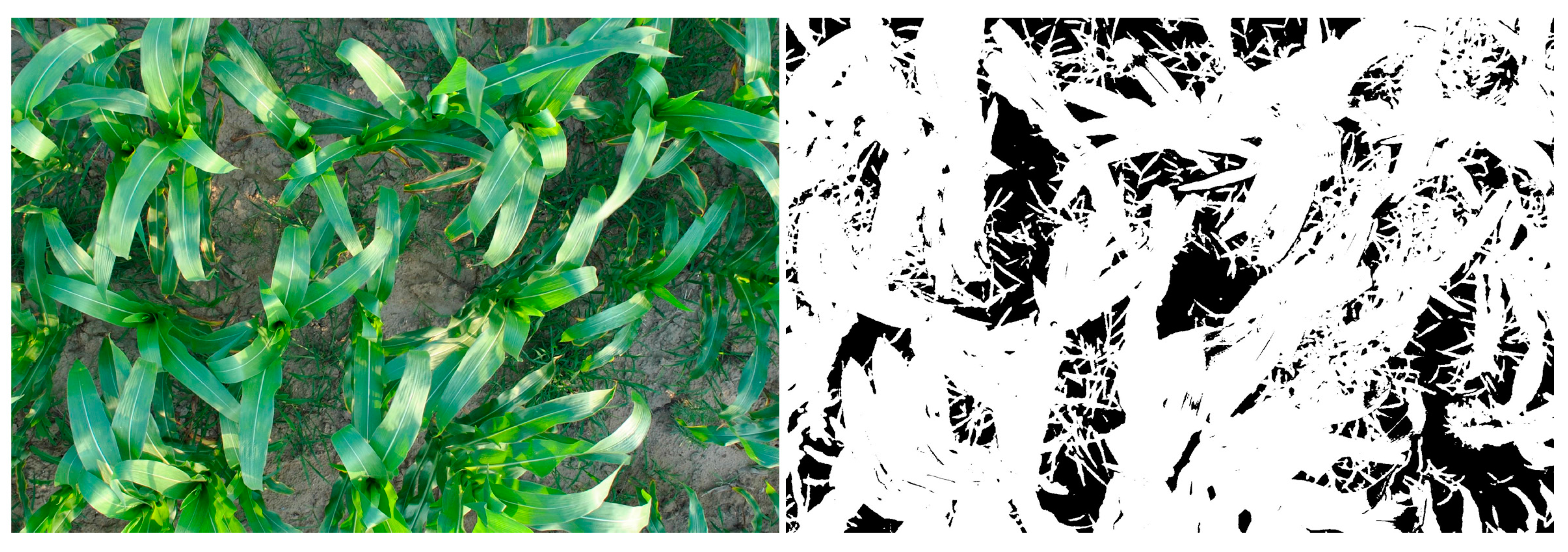
2.3. Field Survey Data

The field survey data were acquired from 25 May to 14 September 2012. Measurements were taken every 5 days before 23 July and every 10 days thereafter [37,38]. To match the acquisition dates of the Landsat 7 ETM+ data, field FVC measurements from 23 June, 10 July, and 28 August were selected. There were 44 valid field FVC measurements that were not located in the stripes of the Landsat 7 ETM+ data, of which 39 were mostly covered by corn, vegetables, orchards and wheat. Five sites were mostly covered by desert vegetation such as camel thorn (Table 1).

The field FVC measurements were conducted using digital photography. The sample sites were designated as 10 m × 10 m for the low vegetation types such as corn and 30 m × 30 m for tall vegetation types such as fruit trees. Nine photos were taken uniformly in every sample site. The photos of low vegetation types were acquired from the nadir with a long stick equipped with a camera at the end. For the tall trees in the orchard, a top-down direction was used to take photos of low vegetation under the tree crown, whereas a bottom-up direction was used to capture the tree crown. The FVC was calculated from each photo, and the average FVC value of the nine photos of each sample site of low vegetation types was considered as the true FVC value of the sample site. As for the orchard sample site, the FVC was calculated using the following equation:

FVC = FVC_up + (1 − FVC_up) × FVC_down

(1)

where FVC_up and FVC_down were FVC values extracted from the photos captured by the bottom-up and top-down directions, respectively.

The FVC of each photo was calculated using an automatic segmentation method [39], which transformed the photos from the RGB color space to the International Commission on Illumination (CIE) L*a*b* color space that could more easily identify the green vegetation pixels. The segmentation method was based on the Gaussian model, which was used to fit a distribution histogram of green vegetation and background pixels in order to find a suitable threshold value to segment the image into green vegetation and non-green vegetation pixels. Then, the percentage of green vegetation pixels for each photo could be obtained as the FVC of this photo. A randomly selected photo taken in the field and the corresponding segmentation of green vegetation and non-green vegetation pixels is shown in Figure 2. It can be seen that the segmentation results were visually satisfactory for FVC extraction from photos in this study.

2.4. Individual FVC Estimation Methods

2.4.1. Pixel Dimidiate Model

The pixel dimidiate model assumes that a pixel is composed of vegetation and non-vegetation compositions [24], and that the FVC can be estimated using Equation (2):

$$\mathrm{FVC}=(\mathrm{S}-{\mathrm{S}}_{\mathrm{soil}})/\left({\mathrm{S}}_{\mathrm{veg}}-{\mathrm{S}}_{\mathrm{soil}}\right)$$

(2)

where S is the spectral response of the remote sensing data; ${\mathrm{S}}_{\mathrm{veg}}$ and ${\mathrm{S}}_{\mathrm{soil}}$ are spectral responses for a pure vegetation pixel and a pure soil pixel, respectively.

The vegetation index (VI), an important indicator for vegetation growth conditions [40,41], is usually used in the pixel dimidiate model as the spectral response of remote sensing data to calculate the FVC. The visible and NIR reflectance are sensitive to vegetation [23,42,43] and can be used to calculate the VIs (NDVI/EVI), which can characterize the vegetation growth conditions and minimize the atmospheric influence [1]. Thus, FVC can be estimated using VI instead of S using Equation (3),

$$\mathrm{FVC}=\left(\mathrm{VI}-{\mathrm{VI}}_{\mathrm{soil}}\right)/\left({\mathrm{VI}}_{\mathrm{veg}}-{\mathrm{VI}}_{\mathrm{soil}}\right)$$

(3)

Both NDVI and EVI were selected to estimate FVC using the dimidiate pixel model [44,45]. NDVI is the most commonly used indicator of vegetation growth, however, it may be saturated when the vegetation coverage is very high. EVI can compensate for the limitation of NDVI for it is sensitive to soil and atmospheric effects. The two VIs are well correlated with leaf area index (LAI), canopy cover, biomass, and the fraction of absorbed photosynthetically active radiation [46,47]. Moreover, EVI can enhance the vegetation information by reducing the influences from atmosphere and background [45,46,48]. For the Landsat 7 ETM+ data, NDVI and EVI are calculated by Equations (4) and (5):

$$\mathrm{NDVI}=\frac{R_{NIR}-R_{Red}}{R_{NIR}+R_{Red}}$$

(4)

$$\mathrm{EVI}=\mathrm{G}\times \left(R_{NIR}-R_{Red}\right)/\left(R_{NIR}+C_1\times R_{Red}-C_2\times R_{Blue}+L\right)$$

(5)

where $R_{Blue}$, $R_{Red}$ and $R_{NIR}$ are the reflectances of the blue, red and NIR bands, respectively. G = 2.5, $C_1$ = 6.0, $C_2$ = 7.5, and L = 1 [49,50,51].

2.4.2. TGDVI Model

The TGDVI model was proposed for FVC estimation based on the reflectance characteristics of vegetation and soil [27]. Furthermore, Jiapaer et al. considered that there were more differences in the reflectances of SWIR, NIR and red bands for Landsat 5 TM data between vegetation and non-vegetation pixels in an arid region [27]. Thus, the authors proposed two modified TGDVI models by replacing the green band by the two SWIR bands of Landsat 5 TM data. The equations of TGDVI and modified TGDVI for Landsat 7 ETM+ data in this study are listed as following:

TGDVI model:

$$d=\frac{R_{NIR}-R_{Red}}{{\lambda }_{NIR}-{\lambda }_{Red}}-\frac{R_{Red}-R_{Green}}{{\lambda }_{Red}-{\lambda }_{Green}}$$

(6)

MTGDVI1 model:

$$d=\frac{R_{NIR}-R_{Red}}{{\lambda }_{NIR}-{\lambda }_{Red}}-\frac{R_{SWIR5}-R_{NIR}}{{\lambda }_{SWIR5}-{\lambda }_{NIR}}$$

(7)

MTGDVI2 model:

$$d=\frac{R_{NIR}-R_{Red}}{{\lambda }_{NIR}-{\lambda }_{Red}}-\frac{R_{SWIR7}-R_{NIR}}{{\lambda }_{SWIR7}-{\lambda }_{NIR}}$$

(8)

$$f_c=\{\begin{array}{c}0 if d\le 0\\ d/d_{veg} if d >0\end{array}$$

(9)

where $R_{Green}$, $R_{NIR}$, $R_{Red}$, $R_{SWIR5}$, and $R_{SWIR7}$ are the reflectance of green, NIR, red and two SWIR bands of Landsat 7 ETM+ data, respectively, and ${\lambda }_{Green}$, ${\lambda }_{NIR}$, ${\lambda }_{Red}$, ${\lambda }_{SWIR5}$, and ${\lambda }_{SWIR7}$ are the corresponding wavelength, respectively. $d_{veg}$ is the d of highly dense vegetation.

2.4.3. Spectral Mixture Analysis

The SMA model is based on the assumption that a pixel’s spectral reflectance is changed by the spectral reflectance of certain endmembers according to a certain function. The linear SMA model assumes that the function is linear, and the general form of the linear SMA is:

$$R_i={\displaystyle \sum }_{j=1}^N\left(f_j{r}_{ij}\right)+ e_i$$

(10)

where $R_i$ is the reflectance for band i (i = 1, 2, 3, 4, 5, 7 for Landsat 7 ETM+ data in this study), N is the number of endmembers, $r_{ij}$ represents the reflectance of endmember j at band i, $f_j$ stands for the fraction of endmember j in the pixel; and $e_i$ is the residual error at band i.

For one pixel, the fractions of all the endmembers are constrained to:

$${\displaystyle \sum }_j^N{f}_j=1and{f}_j\ge 0$$

(11)

and $e_i$ meets the following equation with the least square to minimize the root mean square error (RMSE):

$$\mathrm{RMSE}=\sqrt{{\displaystyle \sum }_{i=1}^N{e}_i/N}$$

(12)

where N is the number of spectral bands.

To estimate FVC using Equation (10), the number of valid bands must be more than the number of endmembers. Because the Landsat 7 ETM+ spectral reflectances of bands 1, 2 and 3 have a strong correlation, the maximum number of endmembers can be four for Landsat 7 ETM+ data estimating FVC using the SMA model [30,52]. Therefore, three endmembers SMA (SMA3) and four endmembers SMA (SMA4) models were investigated in this study. The pixel purity index (PPI) method was used to select the spectral reflectance of endmembers [53,54,55].

Because the pixel dimidiate models, the TGDVI models and the SMA models are all empirical or semi-empirical methods, determination of model parameters plays an important role for FVC estimation. Based on the distribution characteristics of land cover types in the study area, the SMA4 model selects four endmembers including agriculture crops (e.g., corn), orchards, farmland soil and desert soil. The summation of abundances of agriculture crops and orchards was considered to be the FVC of one pixel. Because the spectral responses of agriculture crops and orchards are not so large (Figure 3) and orchards take little part in the study area, SMA3 selects three endmembers including agriculture crops, farmland soil and desert soil, and the abundance of agriculture crops was considered to be the FVC of one pixel. Because the study area may be not large enough, the endmember selection of pure pixels may be difficult. Therefore, to ensure the selected endmembers are pure, the PPI method of endmember selection was performed on the whole Landsat 7 ETM+ data on 12 July when the vegetation was in the most luxuriant period of the three Landsat 7 ETM+ data sets. The spectral responses of the selected 4 endmembers are shown in Figure 3.

2.5. Combination Methods

Different FVC estimation models have their own characteristics which may contain complementary information for improving FVC estimation accuracy. Therefore, combining several individual FVC estimation models may integrate the advantages of individual models and achieve better FVC estimates. Thus, it is necessary to investigate whether the combination methods can generate a better FVC estimation result and to find a feasible combination strategy. Two combination methods, MLR and BMA methods, were evaluated in order to combine different individual FVC estimation models in this study.

2.5.1. The MLR Method

The MLR method is a simple regression method used to obtain the coefficients of each individual FVC estimation method using the least square method. The equation for the MLR method is presented as Equation (13):

$$\mathrm{FVC}={\displaystyle \sum }_{k=1}^K{a}_k\widetilde{f_k}$$

(13)

where FVC is the combined FVC estimation using the MLR method, $a_k$ is the coefficient of FVC estimation from the kth model, K (K = 2, 3, 4, 5, 6, 7) is the number of individual models used in the combination process, and $\widetilde{f_k}$ is the FVC estimation from the kth model. $a_k$ can be estimated using the least square method.

2.5.2. The BMA Method

For the BMA method, the probability density functions (PDFs) for the individual FVC estimation models are weighted by their posterior probability, and the predictive PDF for the combination FVC estimation is a weighted average of the individual models’ PDFs [56,57,58,59]. Therefore, the BMA method combines FVC estimates by adjusting the predictive PDF to achieve a good fit to the field FVC measurements. According to the law of total probability, the predictive PDF, p(y), can be expressed as

$$p(y|f_1,f_2,\dots ,f_K)={\displaystyle \sum }_{k=1}^{K}p(y|f_k)·p(f_k|y^T)$$

(14)

where y is the predictive variable, {$f_1,f_2,\dots ,f_K$} is the ensemble model for variable y, K (K = 2, 3, 4, 5, 6, 7) is the number of the combined model. $p(y|f_k)$ is the predictive PDF when using model $f_k$ alone. $p(f_k|y^T)$ is the posterior probability that model $f_k$ is correct for the given field FVC measurement $y^T$, and can generally be regarded as a statistical weight $w_k$ reflecting how well the model matches the given field survey data, and ${\displaystyle \sum }_{k=1}^K{w}_k=1$. It seems reasonable to assume that the conditional PDF $p(y|f_k)$ meets a normal distribution with a mean $\widetilde{f_k}$ and a standard deviation $\sigma$, that is, $F|f_k~N(\widetilde{f_k}, {\sigma }^2)$. Therefore, the conditional expectation E, which is the predictive FVC of the BMA method combining the FVC estimates from the individual models, can be expressed as:

$$E(y|f_1,f_2,\dots ,f_K)={\displaystyle \sum }_{k=1}^K{w}_k·\widetilde{f_k}$$

(15)

where $\widetilde{f_k}$ is the estimated FVC of the $k$th model.

2.6. Accuracy Assessment

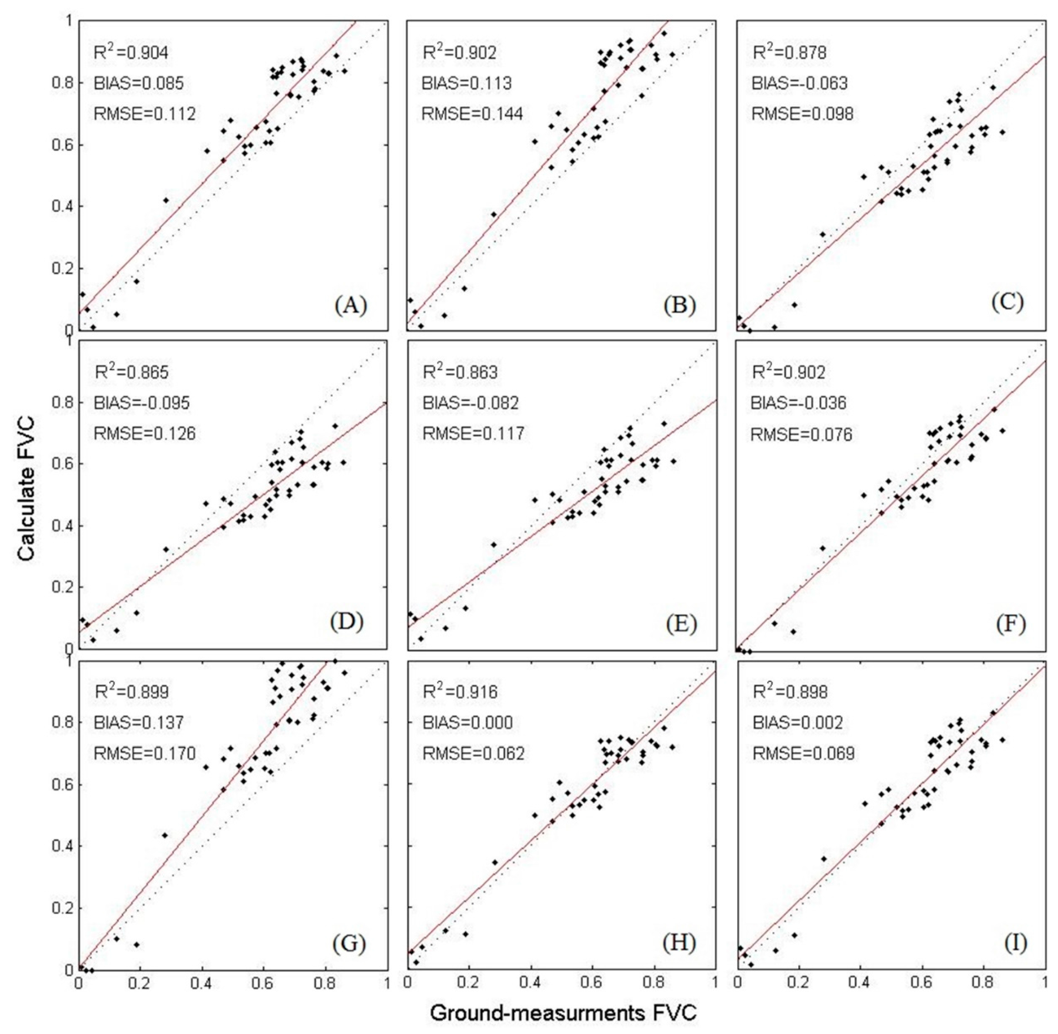
To evaluate the performances of the individual FVC estimation models and those of the combination methods, three regular accuracy assessment indices including the root mean square error, the determination coefficient (R²) and bias, were used in this study. The RMSE was used to measure the deviation between the measured values and the predicted values. R² was an index that measured the linear correlation degree between the measured values and the predicted values. The bias could measure the offset of the estimated results compared with the field survey data as a whole.

3. Results

In the study area, agriculture crops and desert soil were the major vegetation and soil types. The endmembers of agriculture crops and desert soil were regarded as pure vegetation and pure soil pixels in the pixel dimidiate models and the TGDVI models, respectively. Therefore, in the pixel dimidiate models, the ${\mathrm{NDVI}}_{veg}$, ${\mathrm{NDVI}}_{soil}$, ${\mathrm{EVI}}_{veg}$ and ${\mathrm{EVI}}_{soil}$ derived from the spectral reflectances of the endmembers of agriculture crops and desert soil were 0.941, 0.068, 0.919 and 0.066, respectively. Similarly, the spectral reflectance of agriculture crops was used to calculate the parameter $d_{veg}$ in the TGDVI models, and the values of $d_{veg}$ for TGDVI, MTGDVI1 and MTGDVI2 were 3.471, 3.825 and 3.666, respectively.

Figure 4 shows the FVC estimates from the seven individual models and the two combination methods (MLR and BMA) on 10 July 2012, in the most luxuriant period of vegetation. It can be seen that the spatial distribution of FVC was coincident with the actual land cover distribution. The farmland regions presented high FVC values, whereas desert regions presented low FVC values. Comparing the FVC estimates from the individual models and the two combination methods (Figure 4), it can be found that pixel dimidiate models using NDVI (A), EVI (B), and SMA4 (G) had higher FVC values, and the others had lower values in the farmland. In addition, TGDVI models (C, D and E), SMA3 (F) and SMA4 (G) had lower FVC values in the low FVC regions. The MLR (H) and BMA (I) combination methods had similar performances. The result of SMA3 (E) was in the middle level compared to the other six individual models and was similar to the results of the two combination methods. In the northwest part of the farmland, the results from (A) to (E) could distinguish the river from the desert and the farmland, and the river region had very low FVC values because the VIs used in these models could distinguish water from other land cover types. However, the results from SMA3 and SMA4 showed slightly poorer performance in the river region because there was no river endmember selected. The result from the MLR method in this region was also influenced. However, the BMA method performed well in this condition. To obtain more accurate FVC estimates in the SMA models, the water region could be masked before FVC estimation.

The accuracy assessment indices (R², RMSE and bias) of the seven individual models, and the two combination methods (MLR and BMA) were calculated based on field FVC measurements (Figure 5). The accuracy assessment was coincident with Figure 4. For the seven individual models, the pixel dimidiate models using NDVI (A) and EVI (B) had higher R², whereas the FVC estimates were overestimated compared to the field FVC measurements. The bias of the pixel dimidiate model using EVI was higher than that of using NDVI. For the TGDVI models, the ${\mathrm{R}}^2$ and RMSE of MTGDIV1 (D) and MTGDVI2 (E) were higher than that of TGDVI (C), and the biases of the three TGDVI models were negative which indicated that these models underestimated the actual values. In addition, the bias of the TGDVI models became larger when the FVC had larger values. The SMA3 (F) had the best performance of the seven individual models with the lowest RMSE and bias as well as the highest R². On the other hand, the SMA4 (G) model had a relatively poor performance with regards to FVC overestimation compared with the other six models. This result might have been caused by the orchard endmember, which only occupied a small part of the study area. As for the two combination methods, the MLR method had the best performance (R² = 0.913, RMSE = 0.063, bias = 0) compared to the seven individual models and the BMA method. In addition, the BMA method (R² = 0.898, RMSE = 0.069, bias = 0.002) also performed better than the seven individual models. This could indicate that the combination strategies could effectively improve FVC estimation accuracy.

4. Discussion

Different FVC estimation models have their own advantages and complementary information for FVC estimation. The two combination methods can both effectively combine the advantages of each individual model and achieve better FVC estimates. The MLR method obtains the coefficients of each individual model in the combinations, which does not require the summation of the coefficients equal to 1. Therefore, it can combine the results from different models to achieve a better performance even though they are all overestimated or underestimated. Different from the MLR method, BMA method requires the summation of the weights of each individual model equal to 1. Therefore, when the individual models are all overestimated or underestimated, the combination result will still be overestimated or underestimated.

Based on the number and type of individual models used, the combination methods may achieve different FVC estimation results. Therefore, it is important to investigate how many models and which models are suitable to be used in the combination methods in order to achieve a better result.

Table 2. Accuracy performances of different combinations of individual models using the MLR method (K standards for the number of individual models used in the combination method). RMSE is the root mean square error. R² is determination coefficient.

K	NDVI	EVI	TGDVI	MTGDIV1	MTGDVI2	SMA3	SMA4	Sum(${\mathit{a}}_{\mathit{k}}$)	R2	RMSE	Bias
7	0.2032	0.2627	−0.1904	−3.4923	2.8553	2.4834	−1.0023	1.1196	0.9134	0.0629	−0.0008
6	0.1184	0.2576	—	−4.4273	3.6012	2.3678	−0.8536	1.0641	0.9134	0.0629	−0.0009
5	0.305	—	—	−4.8727	4.022	2.412	−0.814	1.0523	0.9133	0.0629	−0.0007
4	0.2533	—	0.1862	—	—	0.2171	0.3434	1.2909	0.912	0.0634	−0.0005
3	—	—	—	−5.5966	4.7892	1.6725	—	0.8651	0.9103	0.064	0.0000
2	0.6726	—	—	—	—	0.2405	—	0.9131	0.9059	0.0658	−0.0021

and

Table 3. Accuracy performances of different combinations of individual models using the BMA method (K standards for the number of individual models used in the combination method).

K	NDVI	EVI	TGDVI	MTGDIV1	MTGDVI2	SMA3	SMA4	Sum(${\mathit{a}}_{\mathit{k}}$)	R2	RMSE	Bias
7	0.1661	0.1198	0.1602	0.1219	0.1324	0.1998	0.0998	1	0.8957	0.0693	0.0016
6	0.1869	0.1364	—	0.1519	0.1651	0.2457	0.1141	1	0.8965	0.0697	0.0102
5	0.1869	0.1364	0.2054	—	0.1705	0.2553	—	1	0.8973	0.0686	−0.0005
4	0.2533	0.1862	—	0.2171	—	0.3434	—	1	0.9001	0.0688	0.0097
3	0.3251	—	0.302	—	—	0.3729	—	1	0.9003	0.0683	−0.005
2	0.418	—	—	—	—	0.582	—	1	0.9043	0.0692	0.0146

show the results using MLR and BMA methods based on different combinations of individual models, when the best accuracy is achieved in a certain number of individual models used. It can be seen that R² increases and RMSE decreases with an increase in the number of individual models used in the MLR method (Table 2). However, the accuracy increase is small when the number of individual models used reaches a certain level. It can be seen that when two suitable models are combined a good performance can be achieved, and adding more models in the MLR method only presents a small improvement. Therefore, it can be concluded that a satisfactory result can be achieved using two suitable individual models and that there is no obvious improvement in accuracy by adding more models to the MRL combination method. Moreover, the coefficients of individual models can be positive or negative and the summation of coefficients in each combination varied from 0.86 to 1.29. Therefore, there is no direct relationship between the summation of coefficients and the accuracy.

As for the BMA combination method, the R² of the combinations is decreased and there is almost no improvement in RMSE as the number K increased (Table 3), which is different from the case of the MLR method. The BMA method can achieve good accuracy when the two individual models, including the pixel dimidiate model using NDVI and the SMA3 model, are combined, and more individual models used in the BMA method cannot improve the FVC estimation accuracy. The coefficients in the BMA method are all positive and the summation of coefficients in each combination is equal to 1. This may be the reason why accuracies are different from those in the MLR method. Therefore, it can be indicated that the BMA method can achieve a satisfactory result when two suitable individual models are used, and the accuracy will slightly decrease when more individual models are used in the combination. Additionally, the pixel dimidiate model using NDVI and the SMA3 model are present in almost all the combinations using the MLR and BMA methods. It can be indicated that the pixel dimidiate model using NDVI and the SMA3 model are two stable methods for FVC estimation in the agriculture region using Landsat 7 ETM+ data.

There are also some potential limitations regarding this study. Firstly, only Landsat 7 ETM+ data were used in this study, whereas the performances of FVC estimation models and the combination methods might be influenced by the remote sensing data according to their technical characteristics such as spatial resolution, spectral bands, and radiometric resolution. Therefore, more remote sensing data from different sensors should be investigated in order to evaluate their performance on FVC estimation in a more complex environment. In addition, only NDVI and EVI were used in the pixel dimidiate model, and more vegetation indices could be used for FVC estimation, such as soil adjusted vegetation index (SAVI) and modified SAVI (MSAVI) [26,60,61]. Therefore, more FVC estimation methods using remote sensing data could be evaluated in future work. Furthermore, the number of validation samples was not large and many of them exhibited an FVC value between 0.4 to 0.8, thus the study was limited to medium-to-high green vegetation cover in an arid area with bright soil. More validation samples covering various vegetation types and growth conditions would be a good complement to this study, which could be future work.

5. Conclusions

This study investigated the performances of several FVC estimation models using Landsat 7 ETM+ data in the oasis of the Heihe region and proposed two combination methods to improve FVC estimation accuracy. Based on the validation results, the following conclusions could be made: (1) the SMA3 achieved the best performance of the individual models for FVC estimation in this study; (2) the MLR and BMA combination methods could both integrate the advantages of individual models and effectively improve FVC estimation accuracy; and (3) satisfactory results could be achieved by combining two appropriate individual models using both MLR and BMA methods, and adding more models in the combination methods had little effect on improving FVC estimation accuracy. Though combination methods can achieve better FVC estimation accuracy, improving individual models and checking the possible generalization of these models is also an important issue for further research.

References

1. Zhang, X.; Liao, C.; Li, J.; Sun, Q. Fractional vegetation cover estimation in arid and semi-arid environments using HJ-1 satellite hyperspectral data. Int. J. Appl. Earth Obs. Geoinf. 2013, 21, 506–512. [Google Scholar] [CrossRef]
2. Jia, K.; Liang, S.; Liu, S.; Li, Y.; Xiao, Z.; Yao, Y.; Jiang, B.; Zhao, X.; Wang, X.; Xu, S.; et al. Global land surface fractional vegetation cover estimation using general regression neural networks from MODIS surface reflectance. IEEE Trans. Geosci. Remote Sens. 2015, 53, 4787–4796. [Google Scholar] [CrossRef]
3. Gitelson, A.A.; Kaufman, Y.J.; Stark, R.; Rundquist, D. Novel algorithms for remote estimation of vegetation fraction. Remote Sens. Environ. 2002, 80, 76–87. [Google Scholar] [CrossRef]
4. Camacho, F.; Cernicharo, J.; Lacaze, R.; Baret, F.; Weiss, M. GEOV1: LAI, FAPAR essential climate variables and FCOVER global time series capitalizing over existing products. Part 2: Validation and intercomparison with reference products. Remote Sens. Environ. 2013, 137, 310–329. [Google Scholar] [CrossRef]
5. Zeng, X.; Dickinson, R.E.; Walker, A.; Shaikh, M.; DeFries, R.S.; Qi, J. Derivation and Evaluation of Global 1-km Fractional Vegetation Cover Data for Land Modeling. J. Appl. Meteorol. 2000, 39, 826–839. [Google Scholar] [CrossRef]
6. Jia, K.; Liang, S.; Zhang, L.; Wei, X.; Yao, Y.; Xie, X. Forest cover classification using Landsat ETM+ data and time series MODIS NDVI data. Int. J. Appl. Earth Obs. Geoinf. 2014, 33, 32–38. [Google Scholar] [CrossRef]
7. Godinez-Alvarez, H.; Herrick, J.E.; Mattocks, M.; Toledo, D.; Van Zee, J. Comparison of three vegetation monitoring methods: Their relative utility for ecological assessment and monitoring. Ecol. Indic. 2009, 9, 1001–1008. [Google Scholar] [CrossRef]
8. Roujean, J.-L.; Lacaze, R. Global mapping of vegetation parameters from POLDER multiangular measurements for studies of surface-atmosphere interactions: A pragmatic method and its validation. J. Geophys. Res. Atmos. 2002, 107, 6–14. [Google Scholar] [CrossRef]
9. Baret, F.; Weiss, M.; Lacaze, R.; Camacho, F.; Makhmara, H.; Pacholcyzk, P.; Smets, B. GEOV1: LAI and FAPAR essential climate variables and FCOVER global time series capitalizing over existing products. Part 1: Principles of development and production. Remote Sens. Environ. 2013, 137, 299–309. [Google Scholar] [CrossRef]
10. Gao, S.; Niu, Z.; Sun, G.; Zhao, D.; Jia, K.; Qin, Y. Height Extraction of Maize Using Airborne Full-Waveform LIDAR Data and a Deconvolution Algorithm. IEEE Geosci. Remote Sens. Lett. 2015, 12, 1978–1982. [Google Scholar]
11. Prince, S.D. Satellite remote sensing of primary production: Comparison of results for Sahelian grasslands 1981–1988. Int. J. Remote Sens. 1991, 12, 1301–1311. [Google Scholar] [CrossRef]
12. McVicar, T.R.; Jupp, D.L.B. The current and potential operational uses of remote sensing to aid decisions on drought exceptional circumstances in Australia: A review. Agric. Syst. 1998, 57, 399–468. [Google Scholar] [CrossRef]
13. Jia, K.; Liang, S.; Gu, X.; Baret, F.; Wei, X.; Wang, X.; Yao, Y.; Yang, L.; Li, Y. Fractional vegetation cover estimation algorithm for Chinese GF-1 wide field view data. Remote Sens. Environ. 2016, 177, 184–191. [Google Scholar] [CrossRef]
14. Ghulam, A.; Qin, Q.; Teyip, T.; Li, Z.-L. Modified perpendicular drought index (MPDI): A real-time drought monitoring method. ISPRS J. Photogramm. Remote Sens. 2007, 62, 150–164. [Google Scholar] [CrossRef]
15. Duveiller, G.; Lopez-Lozano, R.; Cescatti, A. Exploiting the multi-angularity of the MODIS temporal signal to identify spatially homogeneous vegetation cover: A demonstration for agricultural monitoring applications. Remote Sens. Environ. 2015, 166, 61–77. [Google Scholar] [CrossRef]
16. Carlson, T.N.; Ripley, D.A. On the relation between NDVI, fractional vegetation cover, and leaf area index. Remote Sens. Environ. 1997, 62, 241–252. [Google Scholar] [CrossRef]
17. Deardorff, J.W. Efficient prediction of ground surface temperature and moisture, with inclusion of a layer of vegetation. J. Geophys. Res. Oceans 1978, 83, 1889–1903. [Google Scholar] [CrossRef]
18. Dymond, J.R.; Stephens, P.R.; Newsome, P.F.; Wilde, R.H. Percentage vegetation cover of a degrading rangeland from SPOT. Int. J. Remote Sens. 1992, 13, 1999–2007. [Google Scholar] [CrossRef]
19. Purevdorj, T.S.; Tateishi, R.; Ishiyama, T.; Honda, Y. Relationships between percent vegetation cover and vegetation indices. Int. J. Remote Sens. 1998, 19, 3519–3535. [Google Scholar] [CrossRef]
20. Baret, F.; Clevers, J.G.P.W.; Steven, M.D. The robustness of canopy gap fraction estimates from red and near-infrared reflectances: A comparison of approaches. Remote Sens. Environ. 1995, 54, 141–151. [Google Scholar] [CrossRef]
21. Graetz, R.D.; Pech, R.P.; Davis, A.W. The assessment and monitoring of sparsely vegetated rangelands using calibrated Landsat data. Int. J. Remote Sens. 1988, 9, 1201–1222. [Google Scholar] [CrossRef]
22. Gutman, G.; Ignatov, A. The derivation of the green vegetation fraction from NOAA/AVHRR data for use in numerical weather prediction models. Int. J. Remote Sens. 1998, 19, 1533–1543. [Google Scholar] [CrossRef]
23. Price, J.C. Estimating leaf area index from satellite data. IEEE Trans. Geosci. Remote Sens. 1993, 31, 727–734. [Google Scholar] [CrossRef]
24. Case, J.L.; LaFontaine, F.J.; Bell, J.R.; Jedlovec, G.J.; Kumar, S.V.; Peters-Lidard, C.D. A Real-Time MODIS Vegetation Product for Land Surface and Numerical Weather Prediction Models. IEEE Trans. Geosci. Remote Sens. 2014, 52, 1772–1786. [Google Scholar] [CrossRef]
25. Adams, J.B.; Smith, M.O.; Johnson, P.E. Spectral mixture modeling: A new analysis of rock and soil types at the Viking Lander 1 Site. J. Geophys. Res. Solid Earth 1986, 91, 8098–8112. [Google Scholar] [CrossRef]
26. Ding, Y.; Zheng, X.; Zhao, K.; Xin, X.; Liu, H. Quantifying the Impact of NDVIsoil Determination Methods and NDVIsoil Variability on the Estimation of Fractional Vegetation Cover in Northeast China. Remote Sens. 2016, 8, 29. [Google Scholar] [CrossRef]
27. Jiapaer, G.; Chen, X.; Bao, A. A comparison of methods for estimating fractional vegetation cover in arid regions. Agric. For. Meteorol. 2011, 151, 1698–1710. [Google Scholar] [CrossRef]
28. Xiao, J.; Moody, A. A comparison of methods for estimating fractional green vegetation cover within a desert-to-upland transition zone in central New Mexico, USA. Remote Sens. Environ. 2005, 98, 237–250. [Google Scholar] [CrossRef]
29. Okin, G.S. Relative spectral mixture analysis—A multitemporal index of total vegetation cover. Remote Sens. Environ. 2007, 106, 467–479. [Google Scholar] [CrossRef]
30. Theseira, M.A.; Thomas, G.; Sannier, C.A.D. An evaluation of spectral mixture modelling applied to a semi-arid environment. Int. J. Remote Sens. 2002, 23, 687–700. [Google Scholar] [CrossRef]
31. Jiménez-Muñoz, J.; Sobrino, J.; Plaza, A.; Guanter, L.; Moreno, J.; Martinez, P. Comparison Between Fractional Vegetation Cover Retrievals from Vegetation Indices and Spectral Mixture Analysis: Case Study of PROBA/CHRIS Data Over an Agricultural Area. Sensors 2009, 9, 768–793. [Google Scholar] [CrossRef] [PubMed]
32. Camacho-De Coca, F.; García-Haro, F.J.; Gilabert, M.A.; Meliá, J. Vegetation cover seasonal changes assessment from TM imagery in a semi-arid landscape. Int. J. Remote Sens. 2004, 25, 3451–3476. [Google Scholar] [CrossRef]
33. McGwire, K.; Minor, T.; Fenstermaker, L. Hyperspectral Mixture Modeling for Quantifying Sparse Vegetation Cover in Arid Environments. Remote Sens. Environ. 2000, 72, 360–374. [Google Scholar] [CrossRef]
34. Asner, G.P.; Heidebrecht, K.B. Spectral unmixing of vegetation, soil and dry carbon cover in arid regions: Comparing multispectral and hyperspectral observations. Int. J. Remote Sens. 2010, 23, 3939–3958. [Google Scholar] [CrossRef]
35. Baret, F.; Hagolle, O.; Geiger, B.; Bicheron, P.; Miras, B.; Huc, M.; Berthelot, B.; Niño, F.; Weiss, M.; Samain, O.; et al. LAI, fAPAR and fCover CYCLOPES global products derived from VEGETATION. Remote Sens. Environ. 2007, 110, 275–286. [Google Scholar] [CrossRef] [Green Version]
36. Li, X.; Cheng, G.D.; Liu, S.M.; Xiao, Q.; Ma, M.G.; Jin, R.; Che, T.; Liu, Q.H.; Wang, W.Z.; Qi, Y.; et al. Heihe Watershed Allied Telemetry Experimental Research (HiWATER): Scientific Objectives and Experimental Design. Bull. Am. Meteorol. Soc. 2013, 94, 1145–1160. [Google Scholar] [CrossRef]
37. Mu, X.; Huang, S.; Ren, H.; Yan, G.; Song, W.; Ruan, G. Validating GEOV1 Fractional Vegetation Cover Derived From Coarse-Resolution Remote Sensing Images Over Croplands. IEEE J. Sel. Top. Appl. Earth Obs. Remote Sens. 2015, 8, 439–446. [Google Scholar] [CrossRef]
38. Mu, X.; Huang, S.; Chen, Y. HiWATER: Dataset of Fractional Vegetation Cover in the Middle Reaches of the Heihe River Basin; Heihe Plan Science Data Center: LanZhou, China, 2013. [Google Scholar]
39. Liu, Y.; Mu, X.; Wang, H.; Yan, G. A novel method for extracting green fractional vegetation cover from digital images. J. Veg. Sci. 2012, 23, 406–418. [Google Scholar] [CrossRef]
40. Wu, D.; Wu, H.; Zhao, X.; Zhou, T.; Tang, B.; Zhao, W.; Jia, K. Evaluation of Spatiotemporal Variations of Global Fractional Vegetation Cover Based on GIMMS NDVI Data from 1982 to 2011. Remote Sens. 2014, 6, 4217–4239. [Google Scholar] [CrossRef]
41. Jiang, Z.; Huete, A.R.; Chen, J.; Chen, Y.; Li, J.; Yan, G.; Zhang, X. Analysis of NDVI and scaled difference vegetation index retrievals of vegetation fraction. Remote Sens. Environ. 2006, 101, 366–378. [Google Scholar] [CrossRef]
42. Richardson, A.J.; Wiegand, C.L. Comparison of two models for simulating the soil-vegetation composite reflectance of a developing cotton canopy. Int. J. Remote Sens. 1990, 11, 447–459. [Google Scholar] [CrossRef]
43. Price, J.C. Estimating vegetation amount from visible and near infrared reflectances. Remote Sens. Environ. 1992, 41, 29–34. [Google Scholar] [CrossRef]
44. Tucker, C.J. Red and photographic infrared linear combinations for monitoring vegetation. Remote Sens. Environ. 1979, 8, 127–150. [Google Scholar] [CrossRef]
45. Sjöström, M.; Ardö, J.; Arneth, A.; Boulain, N.; Cappelaere, B.; Eklundh, L.; de Grandcourt, A.; Kutsch, W.L.; Merbold, L.; Nouvellon, Y. Exploring the potential of MODIS EVI for modeling gross primary production across African ecosystems. Remote Sens. Environ. 2011, 115, 1081–1089. [Google Scholar] [CrossRef]
46. Gao, X.; Huete, A.R.; Ni, W.; Miura, T. Optical–Biophysical Relationships of Vegetation Spectra without Background Contamination. Remote Sens. Environ. 2000, 74, 609–620. [Google Scholar] [CrossRef]
47. Gurung, R.B.; Breidt, F.J.; Dutin, A.; Ogle, S.M. Predicting Enhanced Vegetation Index (EVI) curves for ecosystem modeling applications. Remote Sens. Environ. 2009, 113, 2186–2193. [Google Scholar] [CrossRef]
48. Huete, A.; Didan, K.; Miura, T.; Rodriguez, E.P.; Gao, X.; Ferreira, L.G. Overview of the radiometric and biophysical performance of the MODIS vegetation indices. Remote Sens. Environ. 2002, 83, 195–213. [Google Scholar] [CrossRef]
49. Walker, J.J.; de Beurs, K.M.; Wynne, R.H. Dryland vegetation phenology across an elevation gradient in Arizona, USA, investigated with fused MODIS and Landsat data. Remote Sens. Environ. 2014, 144, 85–97. [Google Scholar] [CrossRef]
50. Huete, A.; Justice, C.; Liu, H. Development of vegetation and soil indices for MODIS-EOS. Remote Sens. Environ. 1994, 49, 224–234. [Google Scholar] [CrossRef]
51. Huete, A.R.; Liu, H.Q.; Batchily, K.; van Leeuwen, W. A comparison of vegetation indices over a global set of TM images for EOS-MODIS. Remote Sens. Environ. 1997, 59, 440–451. [Google Scholar] [CrossRef]
52. Small, C. Estimation of urban vegetation abundance by spectral mixture analysis. Int. J. Remote Sens. 2001, 22, 1305–1334. [Google Scholar] [CrossRef]
53. Fernández-Manso, A.; Quintano, C.; Roberts, D. Evaluation of potential of multiple endmember spectral mixture analysis (MESMA) for surface coal mining affected area mapping in different world forest ecosystems. Remote Sens. Environ. 2012, 127, 181–193. [Google Scholar] [CrossRef]
54. Rogge, D.M.; Rivard, B.; Zhang, J.; Sanchez, A.; Harris, J.; Feng, J. Integration of spatial–spectral information for the improved extraction of endmembers. Remote Sens. Environ. 2007, 110, 287–303. [Google Scholar] [CrossRef]
55. Qu, L.; Han, W.; Lin, H.; Zhu, Y.; Zhang, L. Estimating Vegetation Fraction Using Hyperspectral Pixel Unmixing Method: A Case Study of a Karst Area in China. IEEE J. Sel. Top. Appl. Earth Obs. Remote Sens. 2014, 7, 4559–4565. [Google Scholar] [CrossRef]
56. Raftery, A.E.; Gneiting, T.; Balabdaoui, F.; Polakowski, M. Using Bayesian Model Averaging to Calibrate Forecast Ensembles. Mon. Weather Rev. 2005, 133, 1155–1174. [Google Scholar] [CrossRef]
57. Yao, Y.; Liang, S.; Li, X.; Hong, Y.; Fisher, J.B.; Zhang, N.; Chen, J.; Cheng, J.; Zhao, S.; Zhang, X.; et al. Bayesian multimodel estimation of global terrestrial latent heat flux from eddy covariance, meteorological, and satellite observations. J. Geophys. Res. Atmos. 2014, 119, 4521–4545. [Google Scholar] [CrossRef]
58. Hoeting, J.A.; Madigan, D.; Raftery, A.E.; Volinsky, C.T. Bayesian model averaging: A tutorial (with comments by M. Clyde, David Draper and E.I. George, and a rejoinder by the authors). Stat. Sci. 1999, 14, 382–417. [Google Scholar]
59. Raftery, A.E.; Madigan, D.; Hoeting, J.A. Bayesian Model Averaging for Linear Regression Models. J. Am. Stat. Assoc. 1997, 92, 179–191. [Google Scholar] [CrossRef]
60. Huete, A.R. A soil-adjusted vegetation index (SAVI). Remote Sens. Environ. 1988, 25, 295–309. [Google Scholar] [CrossRef]
61. Qi, J.; Chehbouni, A.; Huete, A.R.; Kerr, Y.H.; Sorooshian, S. A modified soil adjusted vegetation index. Remote Sens. Environ. 1994, 48, 119–126. [Google Scholar] [CrossRef]
Figure 1. Study area and spatial distribution of the field measurement sites (The field measurement sites were not located in the black stripes).
Remotesensing 09 01121 g001
Figure 2. An example of the photos (Left) taken in the field and the corresponding segmentation (Right) of green vegetation (white) and non-green vegetation pixels (black).
Remotesensing 09 01121 g002
Figure 3. The spectral responses of the selected 4 endmembers for the SMA method.
Remotesensing 09 01121 g003
Figure 4. FVC estimates from the individual models and the two (multiple linear regression (MLR) and Bayesian model averaging (BMA)) combination methods. (A) Pixel dimidiate model using normalized difference vegetation index (NDVI); (B) Pixel dimidiate model using enhanced vegetation index (EVI); (C) three gradient differential vegetation index (TGDVI); (D) modified three gradient differential vegetation index 1 (MTGDIV1); (E) modified three gradient differential vegetation index 2 (MTGDVI2); (F) spectral mixture analysis with three endmembers (SMA3) model and (G) spectral mixture analysis with four endmembers (SMA4) model; (H) MLR method using seven individual models; (I) BMA method using seven individual models.
Remotesensing 09 01121 g004
Figure 5. Accuracy assessment of the individual models and the two (MLR and BMA) combination methods. (A) Pixel dimidiate model using NDVI; (B) Pixel dimidiate model using EVI; (C) TGDVI; (D) MTGDIV1; (E) MTGDVI2; (F) SMA3 model and (G) SMA4 model; (H) MLR method using seven individual models; (I) BMA method using seven individual models.
Remotesensing 09 01121 g005