Evaluation of MERIS Chlorophyll-a Retrieval Processors in a Complex Turbid Lake Kasumigaura over a 10-Year Mission

 ,
, 
 ,
,
Abstract
1. Introduction
2. Methods
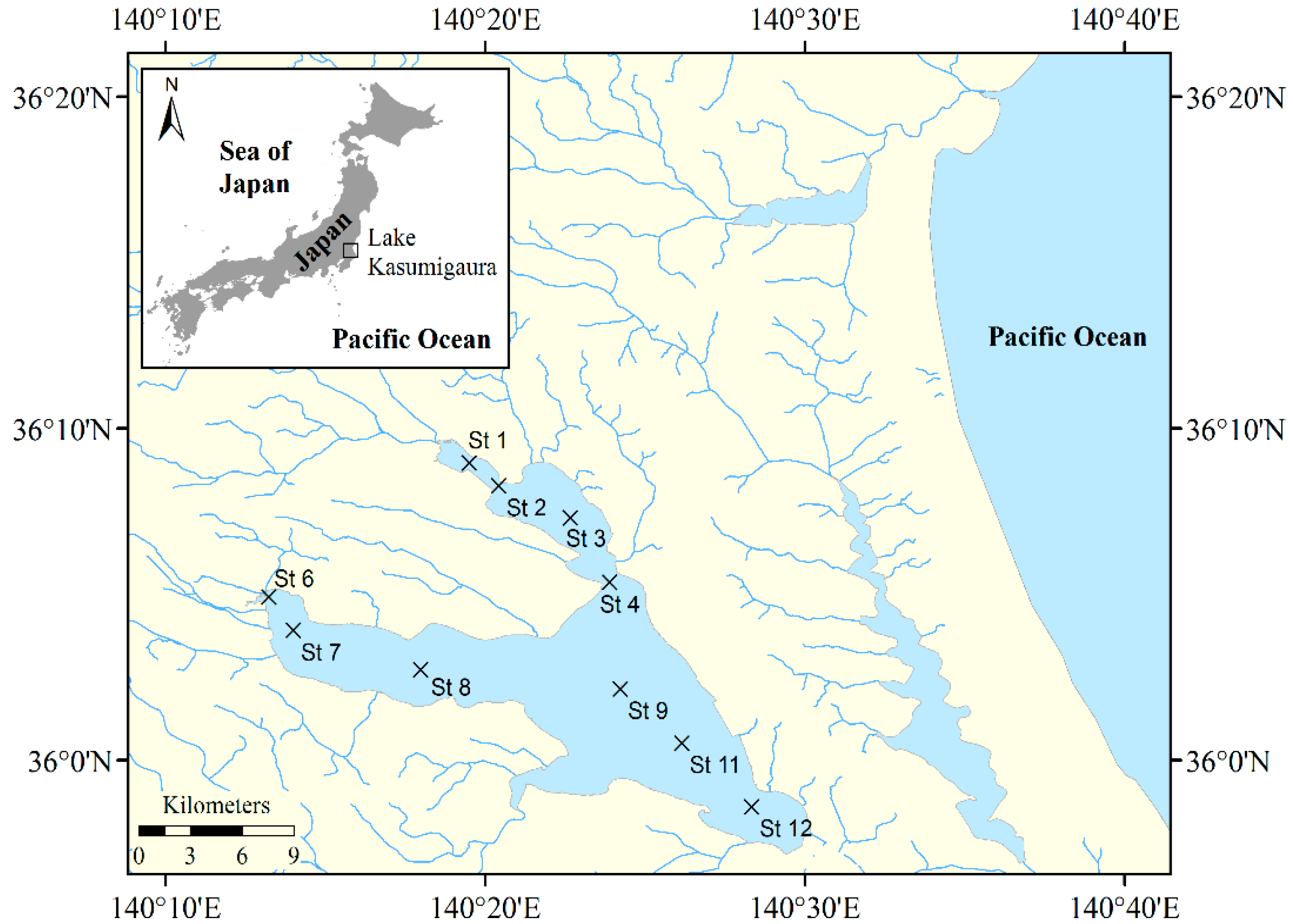
2.1. In Situ Measurements
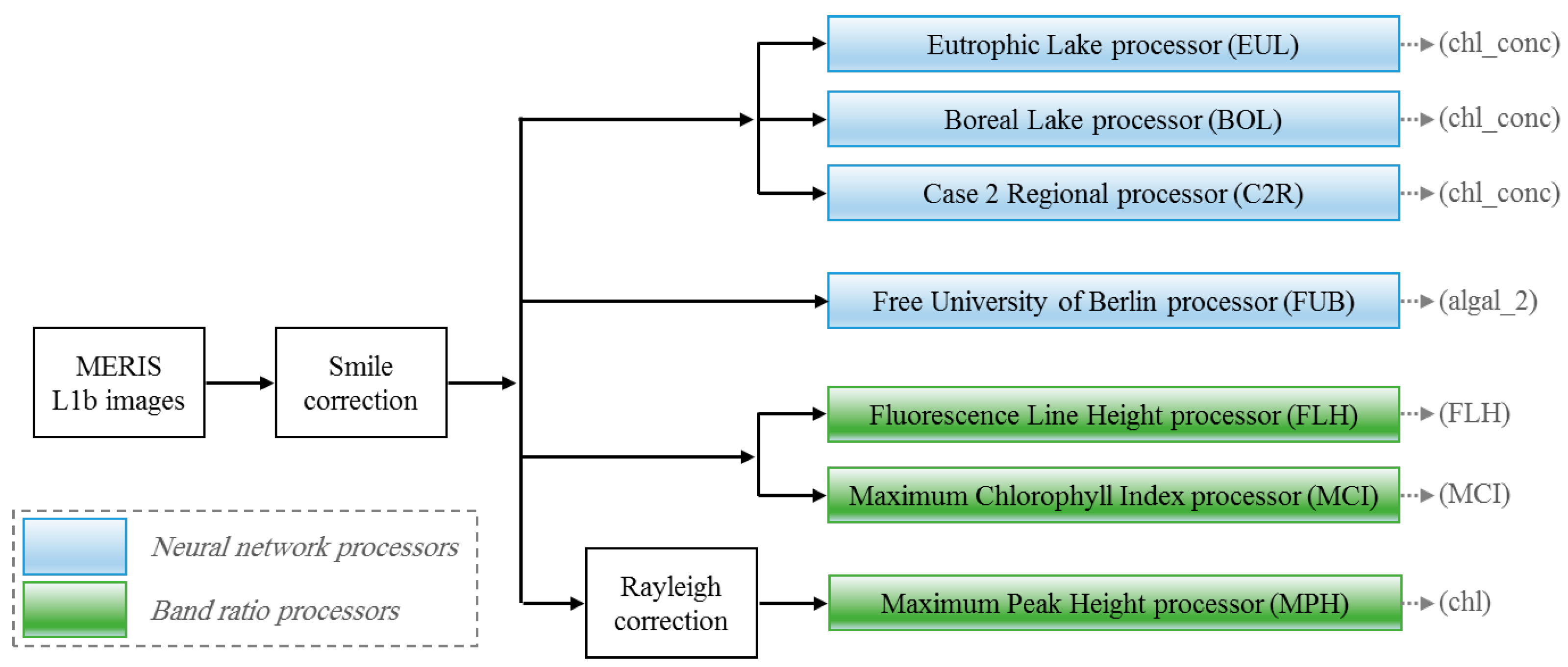
2.2. Medium Resolution Imaging Spectrometer (MERIS) Chlorophyll-a Processors
2.3. MERIS Image Processing
2.4. Accuracy Assessment
3. Results and Discussion
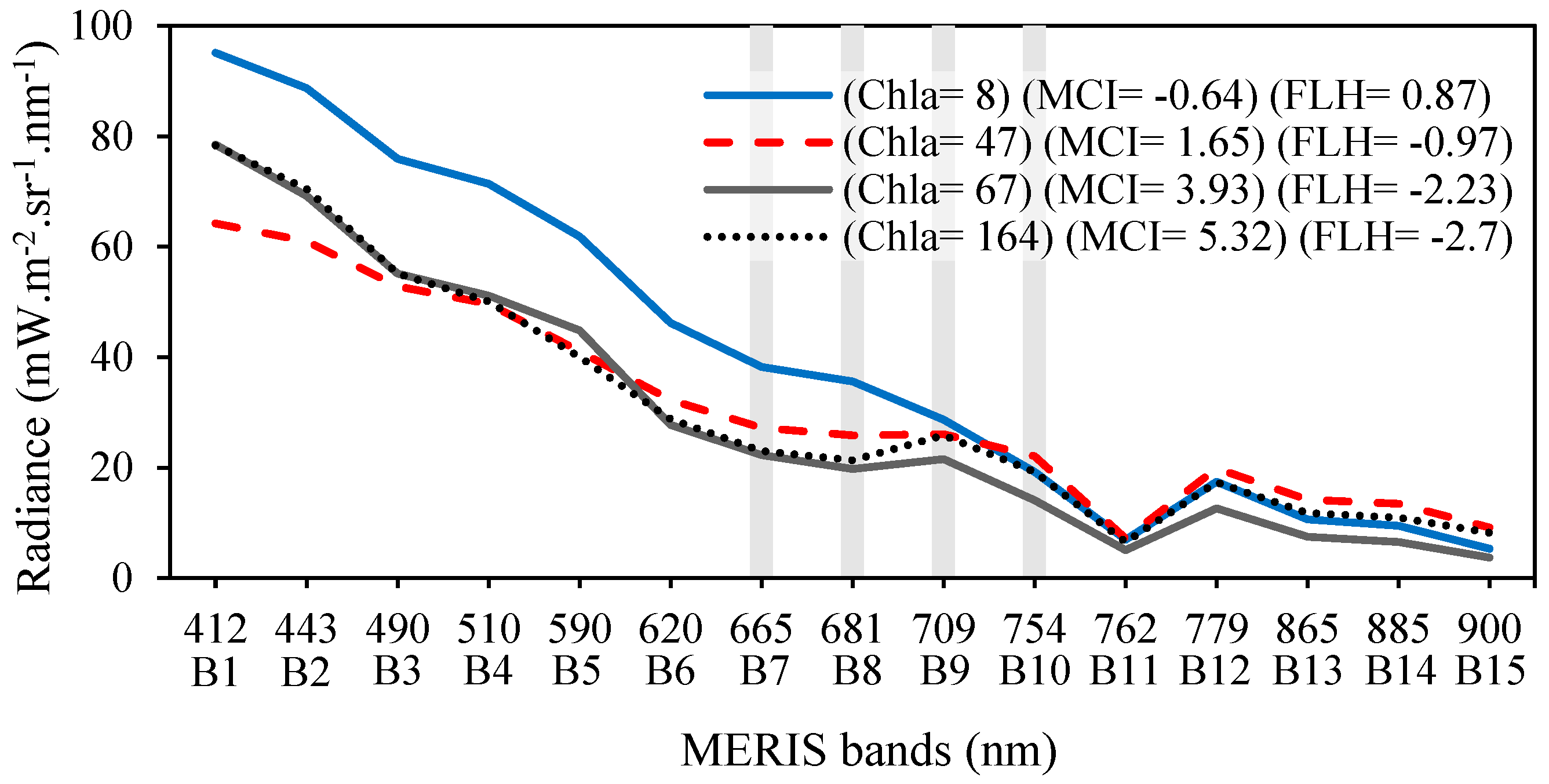
3.1. Characteristics of Synchronized Measurements
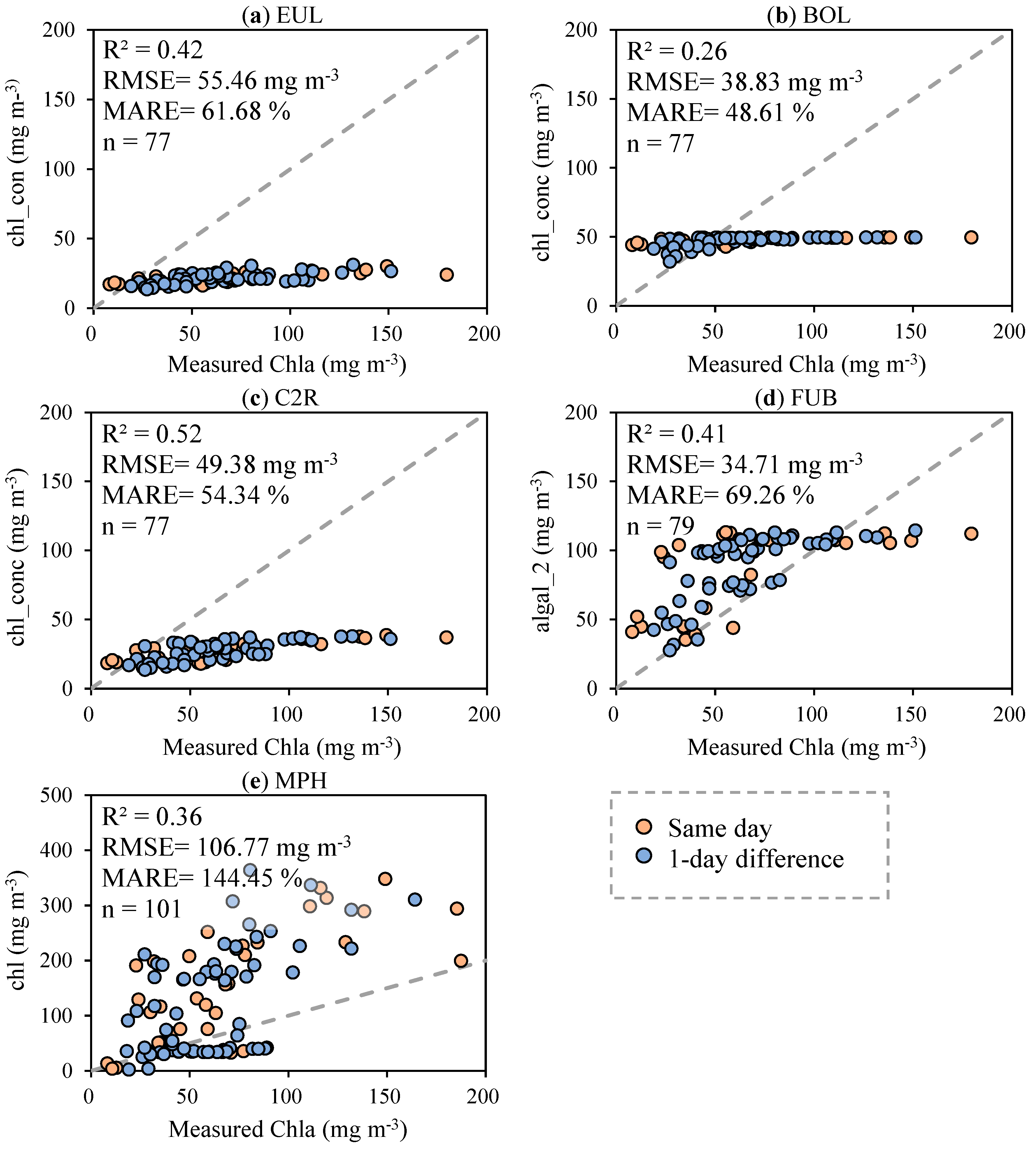
3.2. Evaluation of Chlorophyll-a Retrieval Processors
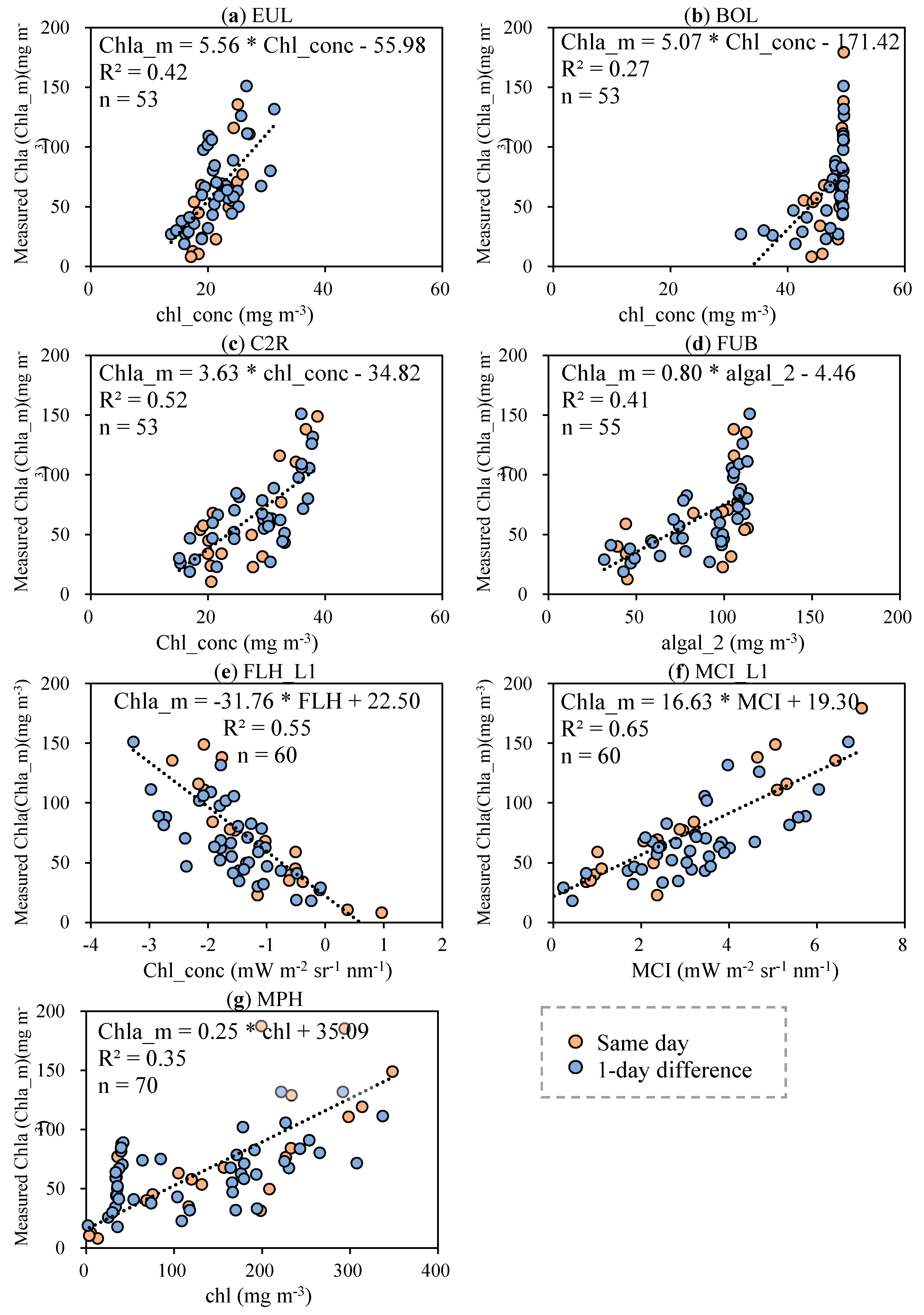
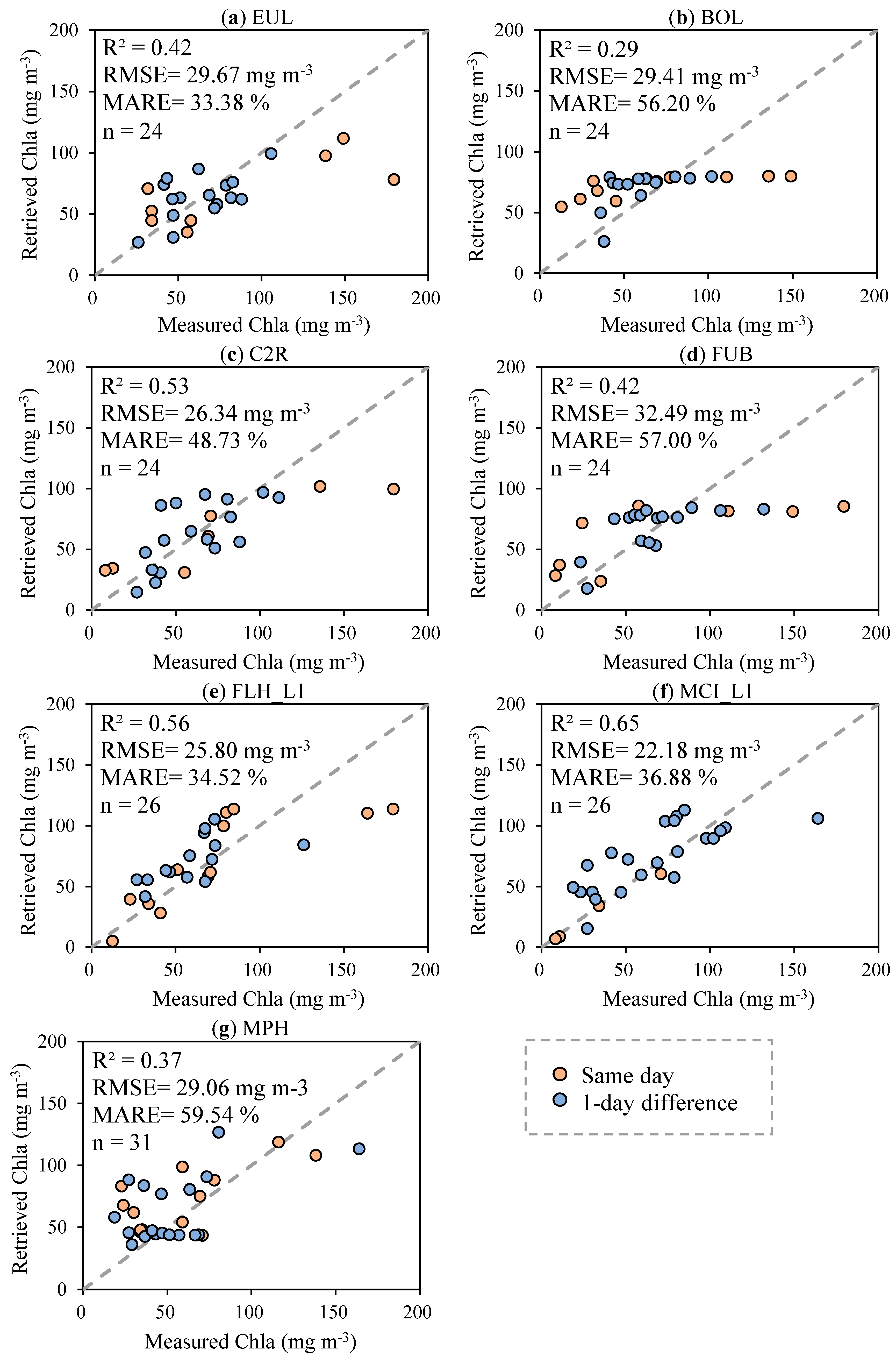
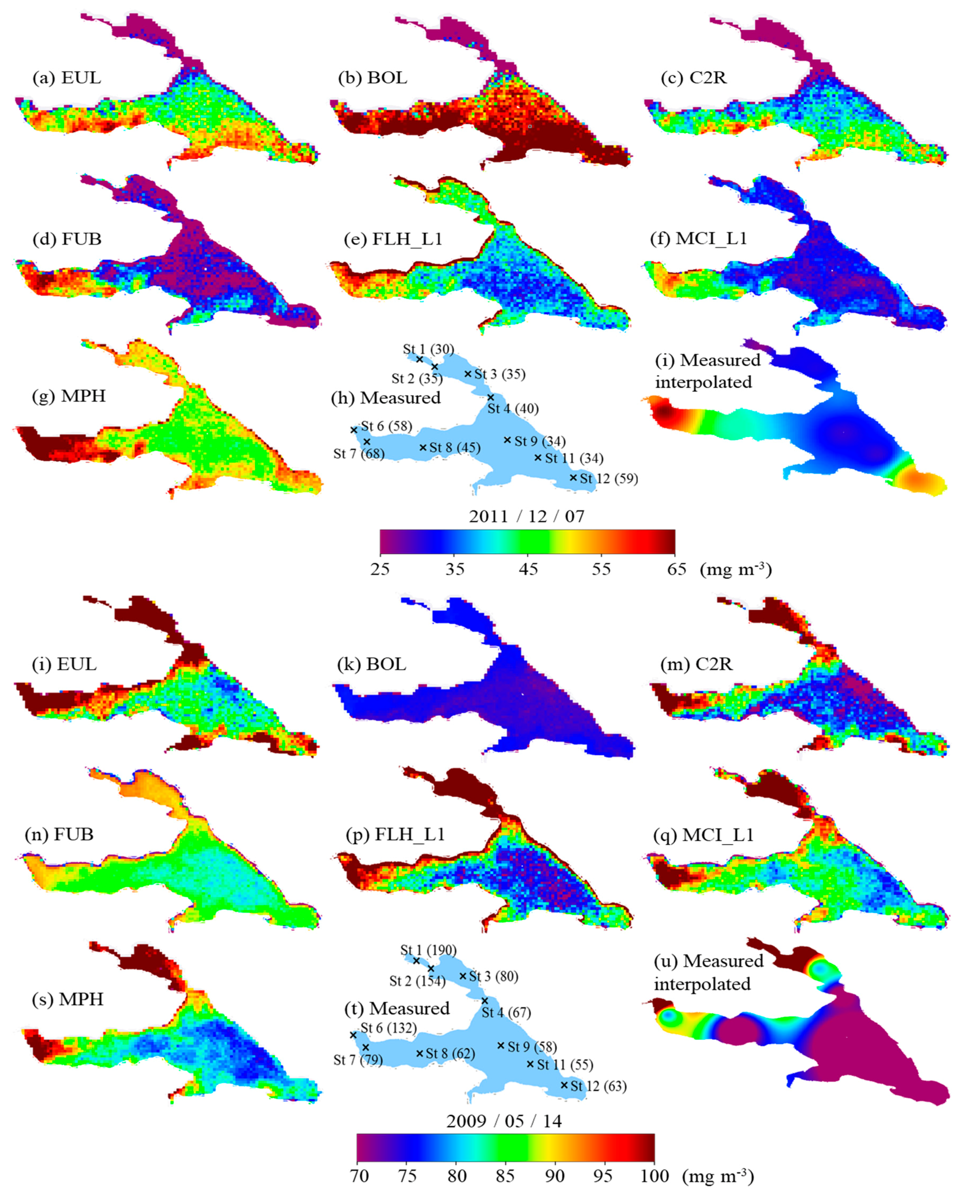
3.3. Processors Adjustment
4. Conclusions
Acknowledgments
Author Contributions
Conflicts of Interest
References
- Gokul, E.A.; Shanmugam, P.; Sundarabalan, B.; Sahay, A.; Chauhan, P. Modelling the inherent optical properties and estimating the constituents’ concentrations in turbid and eutrophic waters. Cont. Shelf Res. 2014, 84, 120–138. [Google Scholar] [CrossRef]
- Dall’Olmo, G.; Gitelson, A.A. Effect of bio-optical parameter variability and uncertainties in reflectance measurements on the remote estimation of chlorophyll-a concentration in turbid productive waters: Modeling results. Appl. Opt. 2006, 45, 3577. [Google Scholar] [CrossRef] [PubMed]
- Oyama, Y.; Matsushita, B.; Fukushima, T.; Matsushige, K.; Imai, A. Application of spectral decomposition algorithm for mapping water quality in a turbid lake (Lake Kasumigaura, Japan) from Landsat TM data. ISPRS J. Photogramm. Remote Sens. 2009, 64, 73–85. [Google Scholar] [CrossRef]
- Su, H.; Liu, H.; Wang, L.; Filippi, A.M.; Heyman, W.D.; Beck, R.A. Geographically Adaptive Inversion Model for Improving Bathymetric Retrieval From Satellite Multispectral Imagery. IEEE Trans. Geosci. Remote Sens. 2014, 52, 465–476. [Google Scholar] [CrossRef]
- Le, C.; Li, Y.; Zha, Y.; Sun, D.; Huang, C.; Zhang, H. Remote estimation of chlorophyll a in optically complex waters based on optical classification. Remote Sens. Environ. 2011, 115, 725–737. [Google Scholar] [CrossRef]
- Gholizadeh, M.H.; Melesse, A.M.; Reddi, L. A Comprehensive Review on Water Quality Parameters Estimation Using Remote Sensing Techniques. Sensors 2016, 16, 1298. [Google Scholar] [CrossRef] [PubMed]
- Gordon, H.R.; Morel, A. Remote Assessment of Ocean Color for Interpretation of Satellite Visible Imagery. In A Review. Lecture Notes on Coastal and Estuarine Studies; Springer: Berlin, Germany, 1983. [Google Scholar]
- Dekker, A.G. Detection of Optical Water Quality Parameters for Eutrophic Waters by High Resolution Remote Sensing; Vrije Universiteit: Amsterdam, The Netherlands, 1993. [Google Scholar]
- Oki, K.; Yasuoka, Y. Estimation of Chlorophyll-a Concentration in Rich Chlorophyll Water Area from Near-infrared and Red Spectral Signature. J. Remote Sens. Soc. Jpn 1996, 16, 315–323. [Google Scholar]
- Gons, H.J. Optical Teledetection of Chlorophyll a in Turbid Inland Waters. Environ. Sci. Technol. 1999, 33, 1127–1132. [Google Scholar] [CrossRef]
- Yoder, J.A.; McClain, C.R.; Blanton, J.O.; Oeymay, L.-Y. Spatial scales in CZCS-chlorophyll imagery of the southeastern U.S. continental shelf. Limnol. Oceanogr. 1987, 32, 929–941. [Google Scholar] [CrossRef]
- Gordon, H.; Brown, J.; Brown, O.; Evans, R.; Smith, R. A semianalytic radiance model of ocean color. J. Geophys. Res. 1988, 93, 10909–10924. [Google Scholar] [CrossRef]
- Matsushita, B.; Yang, W.; Jaelani, L.M.; Setiawan, F.; Fukushima, T. Monitoring Water Quality with Remote Sensing Image Data. In Remote Sensing for Sustainability; CRC Press: Boca Raton, FL, USA, 2016; pp. 163–189. [Google Scholar]
- Austin, R.W.; Petzold, T.J. The determination of the diffuse attenuation coefficient of sea water using the Coastal Zone Color Scanner. In Oceanography from Space; Barale, V., Gower, J.F.R., Alberotanza, L., Eds.; Springer: Boston, MA, USA, 1981; pp. 239–256. [Google Scholar]
- International Ocean Colour Coordinating Group (IOCCG). Remote Sensing of Ocean Colour in Coastal, and Other Optically-Complex, Waters: Reports of the International Ocean Colour Coordinating Group; Sathyendranath, S., Ed.; IOCCG: Dartmouth, NS, Canada, 2000. [Google Scholar]
- Shi, K.; Zhang, Y.; Liu, X.; Wang, M.; Qin, B. Remote sensing of diffuse attenuation coefficient of photosynthetically active radiation in Lake Taihu using MERIS data. Remote Sens. Environ. 2014, 140, 365–377. [Google Scholar] [CrossRef]
- Majozi, N.P.; Salama, M.S.; Bernard, S.; Harper, D.M.; Habte, M.G. Remote sensing of euphotic depth in shallow tropical inland waters of Lake Naivasha using MERIS data. Remote Sens. Environ. 2014, 148, 178–189. [Google Scholar] [CrossRef]
- Ylöstalo, P.; Kallio, K.; Seppälä, J. Absorption properties of in-water constituents and their variation among various lake types in the boreal region. Remote Sens. Environ. 2014, 148, 190–205. [Google Scholar] [CrossRef]
- Kutser, T.; Metsamaa, L.; Strömbeck, N.; Vahtmäe, E. Monitoring cyanobacterial blooms by satellite remote sensing. Estuar. Coast. Shelf Sci. 2006, 67, 303–312. [Google Scholar] [CrossRef]
- Gower, J.; King, S.; Borstad, G.; Brown, L. The importance of a band at 709 nm for interpreting water-leaving spectral radiance. Can. J. Remote Sens. 2008, 34, 287–295. [Google Scholar]
- Gower, J.F.R.; Doerffer, R.; Borstad, G.A. Interpretation of the 685 nm peak in water-leaving radiance spectra in terms of fluorescence, absorption and scattering, and its observation by MERIS. Int. J. Remote Sens. 1999, 20, 1771–1786. [Google Scholar] [CrossRef]
- Gower, J.; King, S.; Borstad, G.; Brown, L. Detection of intense plankton blooms using the 709 nm band of the MERIS imaging spectrometer. Int. J. Remote Sens. 2005, 26, 2005–2012. [Google Scholar] [CrossRef]
- Gower, J.; King, S.; Goncalves, P. Global monitoring of plankton blooms using MERIS MCI. Int. J. Remote Sens. 2008, 29, 6209–6216. [Google Scholar] [CrossRef]
- Matthews, M.W.; Bernard, S.; Robertson, L. An algorithm for detecting trophic status (chlorophyll-a), cyanobacterial-dominance, surface scums and floating vegetation in inland and coastal waters. Remote Sens. Environ. 2012, 124, 637–652. [Google Scholar] [CrossRef]
- Matthews, M.W.; Bernard, S.; Winter, K. Remote sensing of cyanobacteria-dominant algal blooms and water quality parameters in Zeekoevlei, a small hypertrophic lake, using MERIS. Remote Sens. Environ. 2010, 114, 2070–2087. [Google Scholar] [CrossRef]
- Baruah, P.J.; Tamura, M.; Oki, K.; Nishimura, H. Neural network modeling of lake surface chlorophyll and sediment content from Landsat TM imagery. In Proceedings of the Paper Presented at the 22nd Asian Conference on Remote Sensing, Singapore, 5–9 November 2001; Volume 5, p. 9. [Google Scholar]
- Mobley, C.D. Light and Water: Radiative Transfer in Natural Waters; Academic Press: San Diego, CA, USA, 1994. [Google Scholar]
- Doerffer, R.; Schiller, H. MERIS Lake Water Algorithm for BEAM—MERIS Algorithm Theoretical Basis Document; V1.0; GKSS Research Center: Geesthacht, Germany, 2008. [Google Scholar]
- Doerffer, R.; Schiller, H. The MERIS Case 2 water algorithm. Int. J. Remote Sens. 2007, 28, 517–535. [Google Scholar] [CrossRef]
- Schroeder, T.; Schaale, M.; Fischer, J. Retrieval of atmospheric and oceanic properties from MERIS measurements: A new Case-2 water processor for BEAM. Int. J. Remote Sens. 2007, 28, 5627–5632. [Google Scholar] [CrossRef]
- Bresciani, M.; Stroppiana, D.; Odermatt, D.; Morabito, G.; Giardino, C. Assessing remotely sensed chlorophyll-a for the implementation of the Water Framework Directive in European perialpine lakes. Sci. Total Environ. 2011, 409, 3083–3091. [Google Scholar] [CrossRef] [PubMed]
- Jaelani, L.M.; Matsushita, B.; Yang, W.; Fukushima, T. Evaluation of four MERIS atmospheric correction algorithms in Lake Kasumigaura, Japan. Int. J. Remote Sens. 2013, 34, 8967–8985. [Google Scholar] [CrossRef]
- Salem, S.; Higa, H.; Kim, H.; Kazuhiro, K.; Kobayashi, H.; Oki, K.; Oki, T. Multi-Algorithm Indices and Look-Up Table for Chlorophyll-a Retrieval in Highly Turbid Water Bodies Using Multispectral Data. Remote Sens. 2017, 9, 556. [Google Scholar] [CrossRef]
- Ruiz-Verdú, A.; Koponen, S.; Heege, T.; Doerffer, R.; Brockmann, C.; Kallio, K.; Pyhälahti, T.; Peña, R.; Polvorionos, A.; Heblinski, J. Development of MERIS lake water algorithms: Validation results from Europe. In Proceedings of the “2nd MERIS/(A) ATSR User Workshop”, Frascati, Italy, 22–26 September 2008. [Google Scholar]
- Odermatt, D.; Pomati, F.; Pitarch, J.; Carpenter, J.; Kawka, M.; Schaepman, M.; Wüest, A. MERIS observations of phytoplankton blooms in a stratified eutrophic lake. Remote Sens. Environ. 2012, 126, 232–239. [Google Scholar] [CrossRef]
- Binding, C.E.; Greenberg, T.A.; Jerome, J.H.; Bukata, R.P.; Letourneau, G. An assessment of MERIS algal products during an intense bloom in Lake of the Woods. J. Plankton Res. 2011, 33, 793–806. [Google Scholar] [CrossRef]
- Palmer, S.C.J.; Hunter, P.D.; Lankester, T.; Hubbard, S.; Spyrakos, E.; Tyler, N.A.; Présing, M.; Horváth, H.; Lamb, A.; Balzter, H.; et al. Validation of Envisat MERIS algorithms for chlorophyll retrieval in a large, turbid and optically-complex shallow lake. Remote Sens. Environ. 2015, 157, 158–169. [Google Scholar] [CrossRef]
- Higano, Y.; Sawada, T. The Dynamic Optimal Policy to Improve the Water Quality of Lake Kasumigaura. Stud. Reg. Sci. 1995, 26, 75–86. [Google Scholar] [CrossRef]
- NIES Lake Kasumigaura Database, National Institute for Environmental Studies, Japan. Available online: http://db.cger.nies.go.jp/gem/moni-e/inter/GEMS/database/kasumi/index.html (accessed on 12 November 2016).
- CEBES Lake Kasumigaura Database. Interpretations of Observed Data. Available online: http://db.cger.nies.go.jp/gem/moni-e/inter/GEMS/database/kasumi/pdf/methods/interpretation2001.pdf (accessed on 27 June 2017).
- Vollenweider, R.A.; Kerekes, J. Eutrophication of Waters: Monitoring, Assessment and Control; Organisation for Economic Co-operation and Development (OECD): Paris, France, 1982; p. 156. [Google Scholar]
- Hayashi, M.; Ishizaka, J.; Kobayashi, H.; Toratani, M.; Nakamura, T.; NAKASHIMA, Y.; Yamada, S. Evaluation and Improvement of MODIS and SeaWIFS-derived Chlorophyll a Concentration in Ise-Mikawa Bay. J. Remote Sens. Soc. Jpn 2015, 35, 245–259. [Google Scholar]
- DAAC Envisat MEdium Resolution Imaging Spectrometer (MERIS). Available online: https://ladsweb.modaps.eosdis.nasa.gov/missions-and-measurements/meris/ (accessed on 24 August 2017).
- Levrini, G.; Delvart, S. MERIS Product Handbook; European Space Agency (ESA): Paris, France, 2011. [Google Scholar]
- Neville, R.A.; Gower, J.F.R. Passive remote sensing of phytoplankton via chlorophyll α fluorescence. J. Geophys. Res. 1977, 82, 3487–3493. [Google Scholar] [CrossRef]
- Gons, H.J.; Auer, M.T.; Effler, S.W. MERIS satellite chlorophyll mapping of oligotrophic and eutrophic waters in the Laurentian Great Lakes. Remote Sens. Environ. 2008, 112, 4098–4106. [Google Scholar] [CrossRef]
- Fernandez-Jaramillo, A.A.; Duarte-Galvan, C.; Contreras-Medina, L.M.; Torres-Pacheco, I.; de J Romero-Troncoso, R.; Guevara-Gonzalez, R.G.; Millan-Almaraz, J.R. Instrumentation in developing chlorophyll fluorescence biosensing: a review. Sensors 2012, 12, 11853–11869. [Google Scholar] [CrossRef] [PubMed]
- Santer, R.; Carrere, V.; Dubuisson, P.; Roger, J.C. Atmospheric correction over land for MERIS. Int. J. Remote Sens. 1999, 20, 1819–1840. [Google Scholar] [CrossRef]
- Matthews, M.W. Eutrophication and cyanobacterial blooms in South African inland waters: 10years of MERIS observations. Remote Sens. Environ. 2014, 155, 161–177. [Google Scholar] [CrossRef]
- ESA European Space Agency. Earthnet Online. Available online: http://earth.esa.int/ (accessed on 10 March 2015).
- Campbell, G.; Phinn, S.R.; Dekker, A.G.; Brando, V.E. Remote sensing of water quality in an Australian tropical freshwater impoundment using matrix inversion and MERIS images. Remote Sens. Environ. 2011, 115, 2402–2414. [Google Scholar] [CrossRef]
- JMA Monthly Mean Percentage of Possible Sunshine, Mito Station, Japan Meteorological Agency. Available online: http://www.data.jma.go.jp/obd/stats/etrn/view/monthly_s3_en.php?block_no=47629&view=10 (accessed on 4 March 2017).
- ESA MERIS Frequently Asked Questions. Available online: http://earth.esa.int/pub/ESA_DOC/ENVISAT/MERIS/VT-P017-DOC-005-E-01-01_meris.faq.1_1.pdf (accessed on 23 June 2017).
- NLNI Lakes Data, National Land Numerical Information, Japan. Available online: http://nlftp.mlit.go.jp/ksj/ (accessed on 14 March 2017).
- Moore, T.S.; Dowell, M.D.; Bradt, S.; Verdu, A.R. An optical water type framework for selecting and blending retrievals from bio-optical algorithms in lakes and coastal waters. Remote Sens. Environ. 2014, 143, 97–111. [Google Scholar] [CrossRef] [PubMed]
- Salem, S.; Higa, H.; Kim, H.; Kobayashi, H.; Oki, K.; Oki, T. Assessment of Chlorophyll-a Algorithms Considering Different Trophic Statuses and Optimal Bands. Sensors 2017, 17, 1746. [Google Scholar] [CrossRef] [PubMed]
- Palmer, S.C. J.; Odermatt, D.; Hunter, P.D.; Brockmann, C.; Présing, M.; Balzter, H.; Tóth, V.R. Satellite remote sensing of phytoplankton phenology in Lake Balaton using 10 years of MERIS observations. Remote Sens. Environ. 2015, 158, 441–452. [Google Scholar] [CrossRef]
- Hock, R.; Jensen, H. Application of kriging interpolation for glacier mass balance computations. Geogr. Ann. Ser. A Phys. 1999, 81, 611–619. [Google Scholar] [CrossRef]


| Min | Max | Mean | Median | SD | |
|---|---|---|---|---|---|
| Monthly campaign (2002–2012) (n = 1210) | |||||
| Chla (mg∙m−3) | 6.80 | 223.50 | 58.73 | 52.87 | 31.85 |
| TSM (g∙m−3) | 6.30 | 118.30 | 26.80 | 24.30 | 12.22 |
| Same day (n = 39) | |||||
| Chla (mg∙m−3) | 8.10 | 187.40 | 72.97 | 58.90 | 48.77 |
| TSM (g∙m−3) | 11.60 | 47.75 | 24.51 | 25.00 | 8.43 |
| 1-day difference (n = 73) | |||||
| Chla (mg∙m−3) | 18.00 | 164.07 | 65.72 | 63.23 | 31.75 |
| TSM (g∙m−3) | 10.70 | 71.20 | 25.71 | 23.60 | 11.41 |
| Band | Band Center (nm) | Bandwidth (nm) |
|---|---|---|
| B1 | 412.5 | 10 |
| B2 | 442.5 | 10 |
| B3 | 490 | 10 |
| B4 | 510 | 10 |
| B5 | 560 | 10 |
| B6 | 620 | 10 |
| B7 | 665 | 10 |
| B8 | 681.25 | 7.5 |
| B9 | 708.75 | 10 |
| B10 | 753.75 | 7.5 |
| B11 | 760.625 | 3.75 |
| B12 | 778.75 | 15 |
| B13 | 865 | 20 |
| B14 | 88 | 10 |
| B15 | 900 | 10 |
| Processors | ||||
|---|---|---|---|---|
| EUL | BOL | C2R | FUB | |
| apig (443) (m−1) | 0.0318–3.816 | 0.024–0.84 | 0.001–2 | |
| Chla to apig relation | Chla = 31.447 ×apig | Chla = 62.6 ×apig1.29 | Chla = 21 ×apig1.04 | |
| Chla (mg∙m−3) | 1–120 | 0.5–50 | 0.016–43.181 | 0.05–50 |
| bTSM (443) (m−1) | 0.25–30 | 0.96–19.194 | 0.005–30 | |
| TSM to bTSM relation | TSM = 1.7 × bTSM | TSM = 1.042 × bTSM | TSM = 1.73 × bTSM | |
| TSM (mg∙m−3) | 0.425–51 | 0.1–20 | 0.0087–51.9 | 0.05–50 |
| aCDOM (443) (m−1) | 0.1–3 | 0.25–10 | 0.005–5 | 0.005–1 |
| Optical data origin | Spanish lakes | Finnish lakes | North Sea, Baltic Sea, Mediterranean Sea and North Atlantic | |
| Reference | Doerffer et al. [28] | Doerffer et al. [28] | Doerffer et al. [29] | Schroeder et al. [30] |
| 2002 | 2003 | 2004 | 2005 | 2006 | 2007 | 2008 | 2009 | 2010 | 2011 | 2012 | |
|---|---|---|---|---|---|---|---|---|---|---|---|
| January | 1 | 3 | 2 | 5 | 2 | ||||||
| February | 1 | 2 | 4 | 1 | 3 | 1 | |||||
| March | 2 | 4 | 3 | 2 | 3 | 1 | 1 | ||||
| April | 2 | 1 | 3 | 2 | 2 | 6 | 1 | ||||
| May | 2 | 2 | 4 | 4 | 1 | ||||||
| June | 2 | 1 | 2 | 2 | 1 | ||||||
| July | 4 | 1 | |||||||||
| August | 1 | 1 | 1 | 2 | 1 | ||||||
| September | 1 | 1 | |||||||||
| October | 1 | 1 | 2 | 2 | 3 | 1 | |||||
| November | 1 | 3 | 2 | ||||||||
| December | 1 | 1 | 1 | 2 | 2 | 1 | 2 | 4 |
| 2002 | 2003 | 2004 | 2005 | 2006 | 2007 | 2008 | 2009 | 2010 | 2011 | 2012 | |
|---|---|---|---|---|---|---|---|---|---|---|---|
| January | 1 * | 1 * | |||||||||
| February | 1 * | ||||||||||
| March | 1 | ||||||||||
| April | 1 * | ||||||||||
| May | 1 | 1 * | |||||||||
| June | |||||||||||
| July | 1 | ||||||||||
| August | 1 * | 1 * | |||||||||
| September | |||||||||||
| October | 1 | ||||||||||
| November | 1 * | ||||||||||
| December | 1 |
| Processors | Calibration | Validation | |||||
|---|---|---|---|---|---|---|---|
| n | R2 | b | n | R2 | RMSE | MARE | |
| Current study | (Chla in ranges of 8.10–187.40 mg∙m−3) (Lake Kasumigaura, Japan) | ||||||
| EUL | 53 | 0.42 | Chla_m = 5.56 × Chl_conc − 55.98 | 24 | 0.42 | 29.67 | 33.38 |
| BOL | 53 | 0.27 | Chla_m = 5.07 × Chl_conc − 171.42 | 24 | 0.29 | 29.41 | 56.20 |
| C2R | 53 | 0.52 | Chla_m = 3.63 × chl_conc − 34.82 | 24 | 0.53 | 26.34 | 48.73 |
| FUB | 55 | 0.41 | Chla_m = 0.80 × algal_2 − 4.46 | 24 | 0.42 | 32.49 | 57.00 |
| FLH_L1 | 60 | 0.55 | Chla_m = −31.76 × FLH + 22.50 | 26 | 0.56 | 25.80 | 34.52 |
| MCI_L1 | 60 | 0.65 | Chla_m = 16.63 × MCI + 19.30 | 26 | 0.65 | 22.18 | 36.88 |
| MPH | 70 | 0.35 | Chla_m = 0.25 × chl + 35.09 | 31 | 0.37 | 29.06 | 59.54 |
| Ruiz-Verdú et al. (2008) | (Chla < 8 mg∙m−3) (Eleven lakes in Finland, Germany and Spain) | ||||||
| EUL | 16 | --- | Chla_m = 1.26 × Chl_conc + 0.55 | --- | 0.46 | 2.54 | --- |
| BOL | 16 | --- | Chla_m = 2.65 × Chl_conc − 1.79 | --- | 0.38 | 6.74 | --- |
| C2R | 16 | --- | Chla_m = 2.21 × Chl_conc − 1.39 | --- | 0.57 | 4.21 | --- |
| Binding et al. (2011) | (Chla in ranges of 1.9–70.50 mg∙m−3) (Lake of the Woods, Canada) | ||||||
| EUL | 16 | 0.188 | Chla_m = −0.129 × Chl_conc + 17.678 | 12 | --- | 46.24 | --- |
| BOL | 16 | 0.207 | Chla_m = 0.444 × Chl_conc + 7.566 | 12 | --- | 11.84 | --- |
| C2R | 16 | 0.159 | Chla_m = 0.664 × Chl_conc + 7.133 | 12 | --- | 11.15 | --- |
| MCI_L1 | 17 | 0.739 | Chla_m = 6.166 × MCI + 6.347 | 11 | --- | 5.71 | --- |
| Odermatt et al. (2012) | (Chla in ranges of 5–40 mg∙m−3) (Greifensee Lake, Swiss) | ||||||
| EUL | 16 | 0.41 | Chla_m = 12.20 × Chl_conc − 3.17 | --- | --- | --- | --- |
| C2R | 16 | 0.40 | Chla_m = 7.87 × Chl_conc − 2.92 | --- | --- | --- | --- |
| FUB | 16 | 0.39 | Chla_m = 1.27 × algal_2 + 4.70 | --- | --- | --- | --- |
| Lankester et al. (2015) | (Chla in ranges of 1.50–57.00 mg∙m−3) (Lake Balaton, Hungary) | ||||||
| EUL | 118 | 0.42 | Chla_m = 2.01 × Chl_conc − 0.57 | 50 | 0.33 | 6.85 | --- |
| BOL | 91 | 0.46 | Chla_m = 0.65 × Chl_conc + 3.25 | 39 | 0.48 | 9.25 | --- |
| C2R | 116 | 0.46 | Chla_m = 1.63 × Chl_conc + 1.09 | 50 | 0.43 | 7.53 | --- |
| FUB | 76 | 0.32 | Chla_m = 0.30 × algal_2 + 4.63 | 32 | 0.65 | 3.83 | --- |
| FLH_L1 | 141 | 0.78 | Chla_m = −8.08 × FLH + 10.33 | 60 | 0.87 | 4.19 | --- |
| MCI_L1 | 141 | 0.62 | Chla_m = 3.91 × MCI + 11.31 | 60 | 0.69 | 6.62 | --- |
© 2017 by the authors. Licensee MDPI, Basel, Switzerland. This article is an open access article distributed under the terms and conditions of the Creative Commons Attribution (CC BY) license (http://creativecommons.org/licenses/by/4.0/).
Share and Cite
Salem, S.I.; Strand, M.H.; Higa, H.; Kim, H.; Kazuhiro, K.; Oki, K.; Oki, T. Evaluation of MERIS Chlorophyll-a Retrieval Processors in a Complex Turbid Lake Kasumigaura over a 10-Year Mission. Remote Sens. 2017, 9, 1022. https://doi.org/10.3390/rs9101022
Salem SI, Strand MH, Higa H, Kim H, Kazuhiro K, Oki K, Oki T. Evaluation of MERIS Chlorophyll-a Retrieval Processors in a Complex Turbid Lake Kasumigaura over a 10-Year Mission. Remote Sensing. 2017; 9(10):1022. https://doi.org/10.3390/rs9101022
Chicago/Turabian StyleSalem, Salem Ibrahim, Marie Hayashi Strand, Hiroto Higa, Hyungjun Kim, Komatsu Kazuhiro, Kazuo Oki, and Taikan Oki. 2017. "Evaluation of MERIS Chlorophyll-a Retrieval Processors in a Complex Turbid Lake Kasumigaura over a 10-Year Mission" Remote Sensing 9, no. 10: 1022. https://doi.org/10.3390/rs9101022
APA StyleSalem, S. I., Strand, M. H., Higa, H., Kim, H., Kazuhiro, K., Oki, K., & Oki, T. (2017). Evaluation of MERIS Chlorophyll-a Retrieval Processors in a Complex Turbid Lake Kasumigaura over a 10-Year Mission. Remote Sensing, 9(10), 1022. https://doi.org/10.3390/rs9101022