Structure-from-Motion Using Historical Aerial Images to Analyse Changes in Glacier Surface Elevation

Abstract
1. Introduction
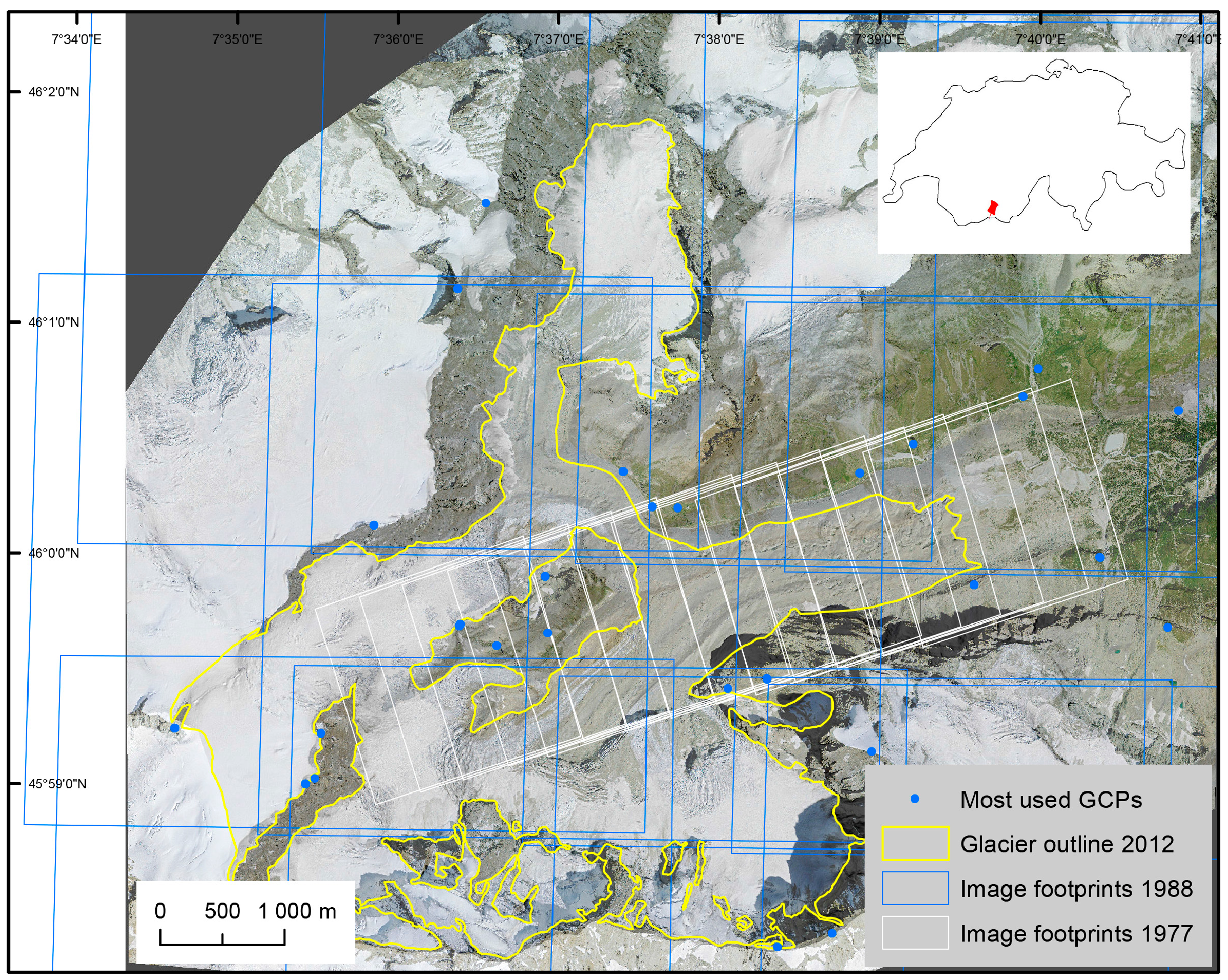
2. Study Area
3. Data and Methods
3.1. Target Imagery
3.2. Reference Data
3.3. Conventional Photogrammetry Using ERDAS-IP 2015
- (1)
- Defining the camera model: Information about the sensor and from the camera calibration report are used to set camera parameters and flying height and delineate the single images;
- (2)
- Performing the bundle adjustment: GCPs are manually located in all images, followed by an automatic calculation of tie points and the subsequent aerotriangulation, including adjustments of previously set camera parameters;
- (3)
3.4. SfM-MVS
- (1)
- Matching the input images: In contrast to conventional photogrammetry, the processing starts with the image matching, which is applied to the raw, unstructured images. Key points are detected in the images that are stable under viewpoint and lighting conditions and are described in relation to their neighbourhood (e.g., using the Scale-invariant feature transform algorithm; [25]). Following this, the algorithm extracts information on the correspondences of these key points in the different images.
- (2)
- Performing the bundle adjustment: This step runs analogous to step (2) of conventional photogrammetry. The calculation of camera parameters can be supported by the input of GCPs; highest accuracy is retrieved with a homogeneous spatial distribution.
- (3)
3.5. Ground Control Points
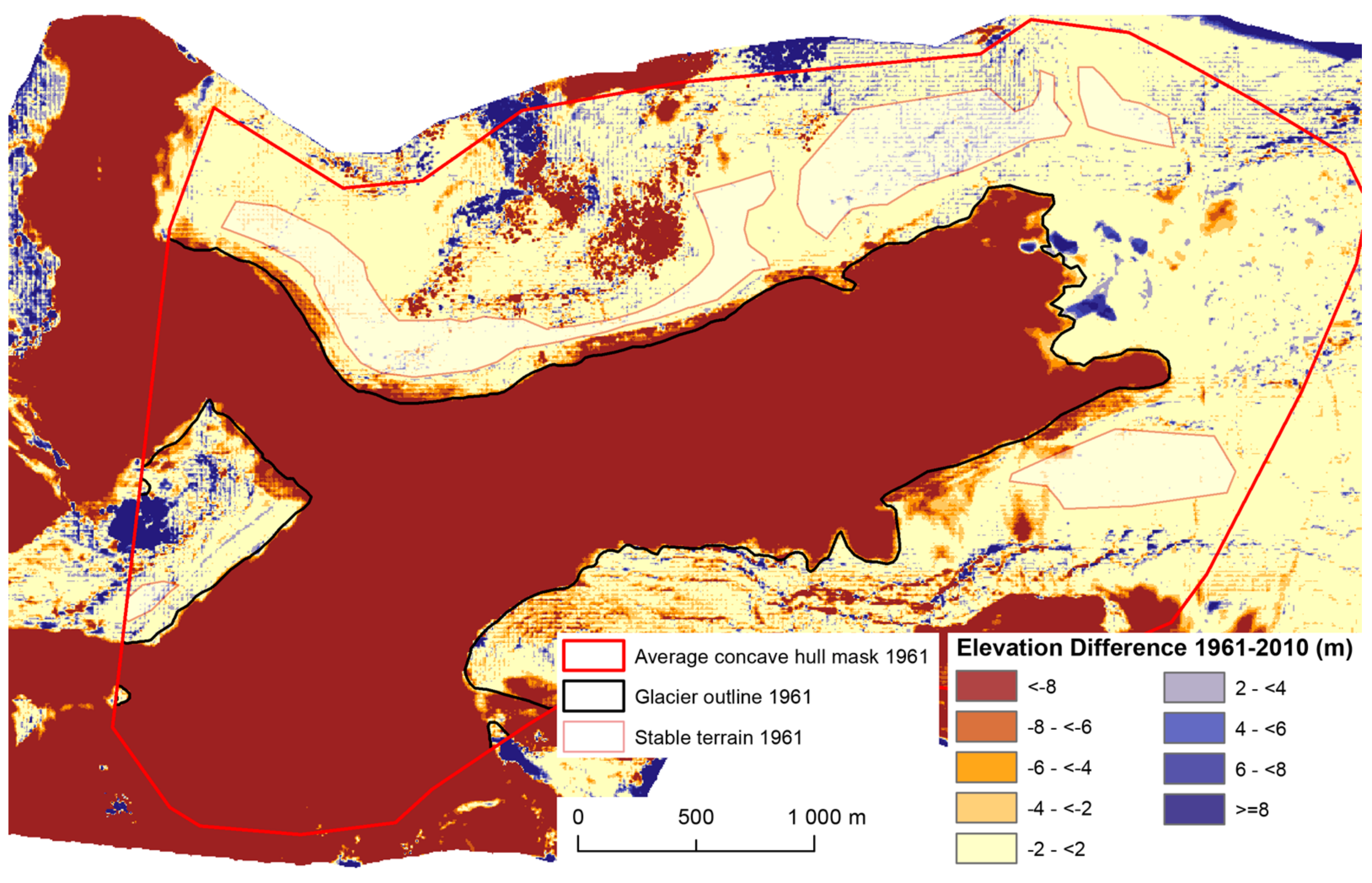
3.6. Final DTM
3.7. Coregistration
3.8. Quality Estimation
4. Results
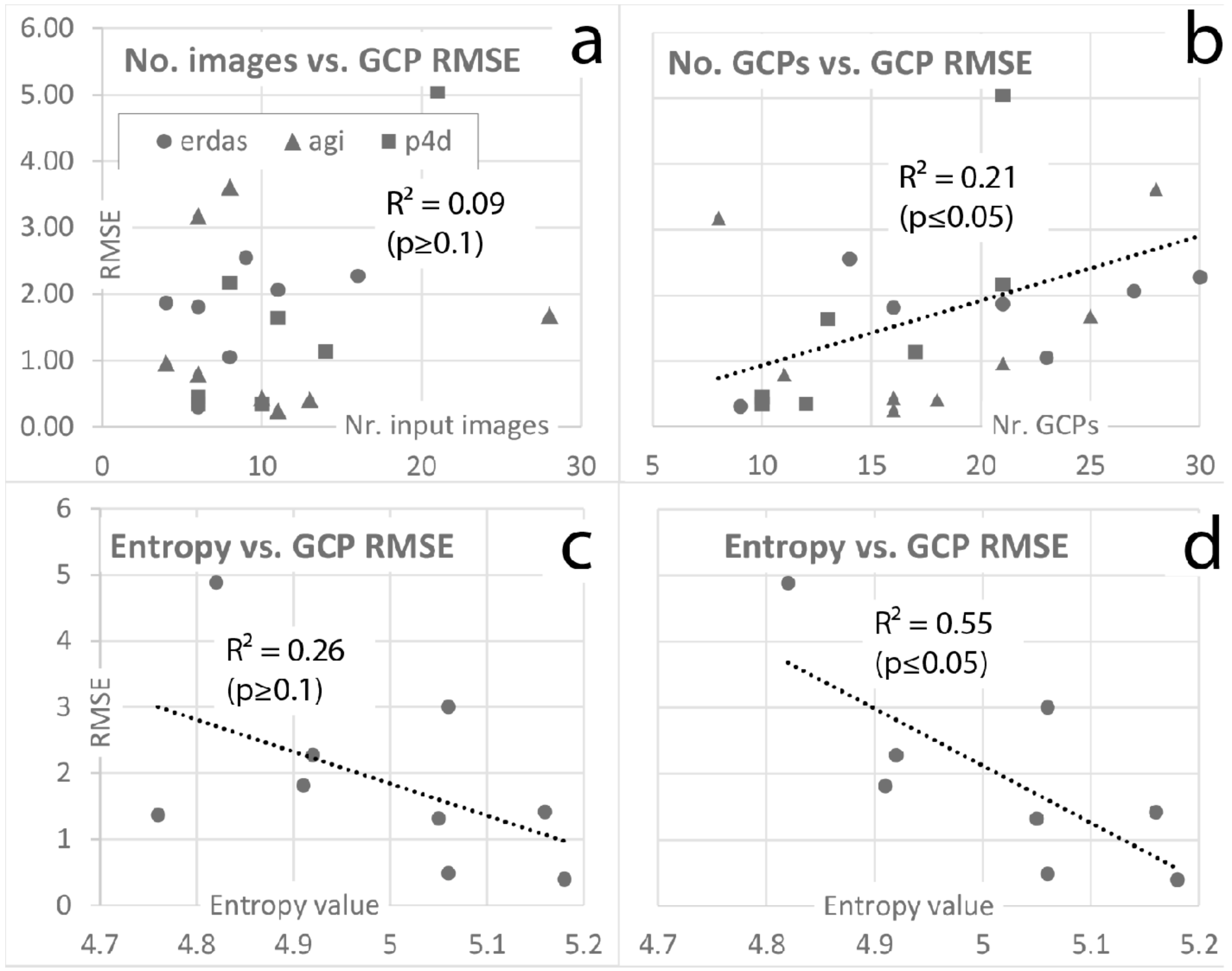
4.1. Bundle Adjustment
4.2. DTM Quality over Stable Terrain
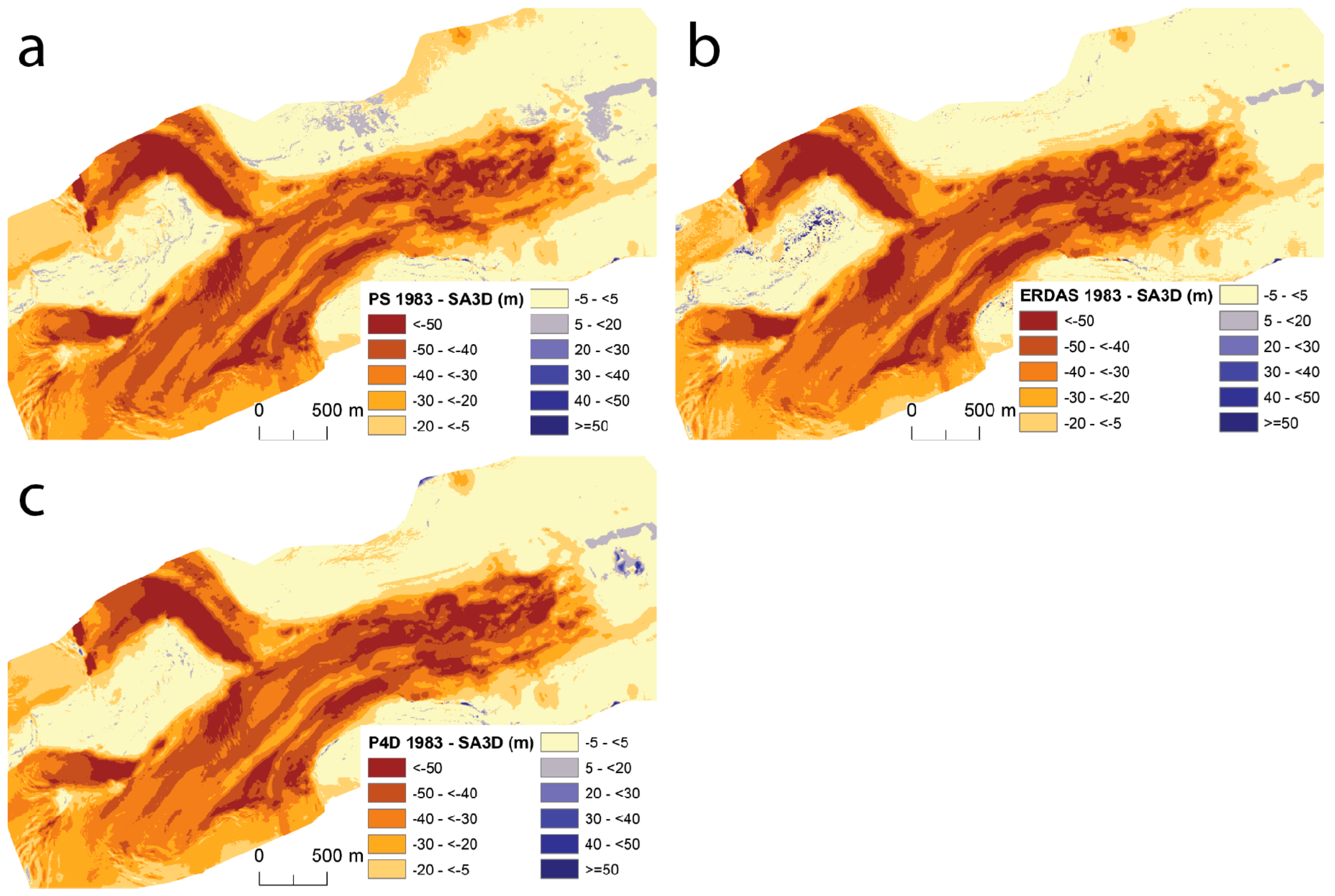
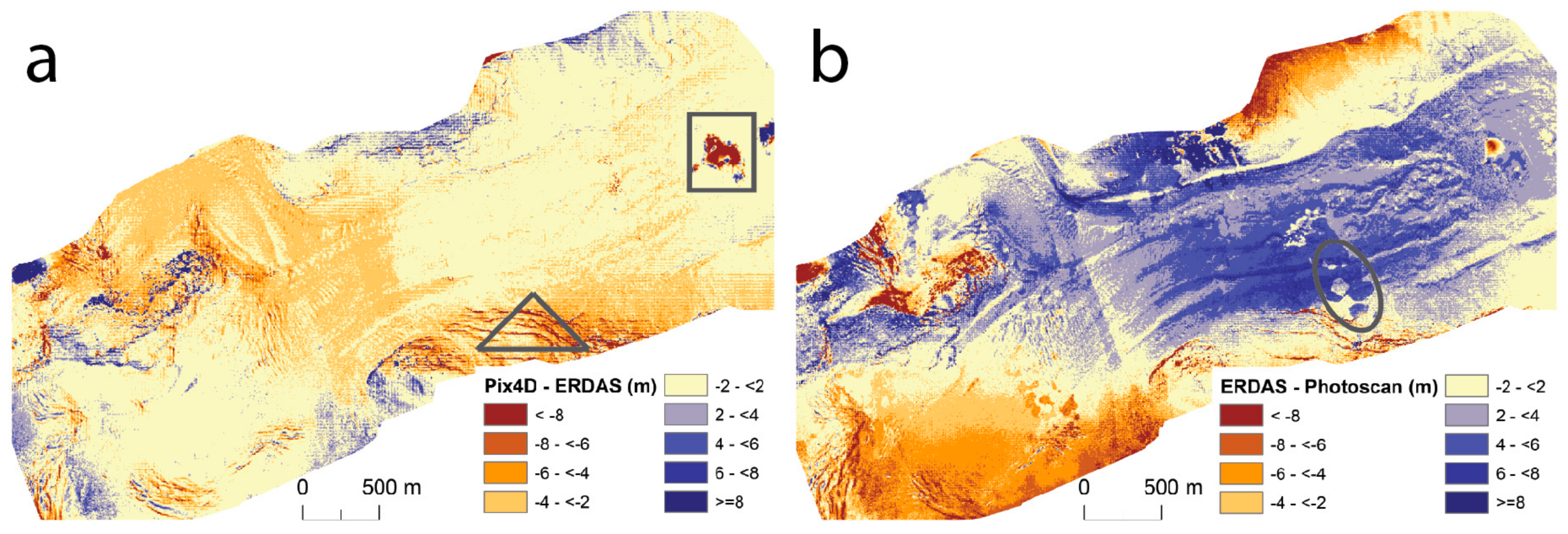
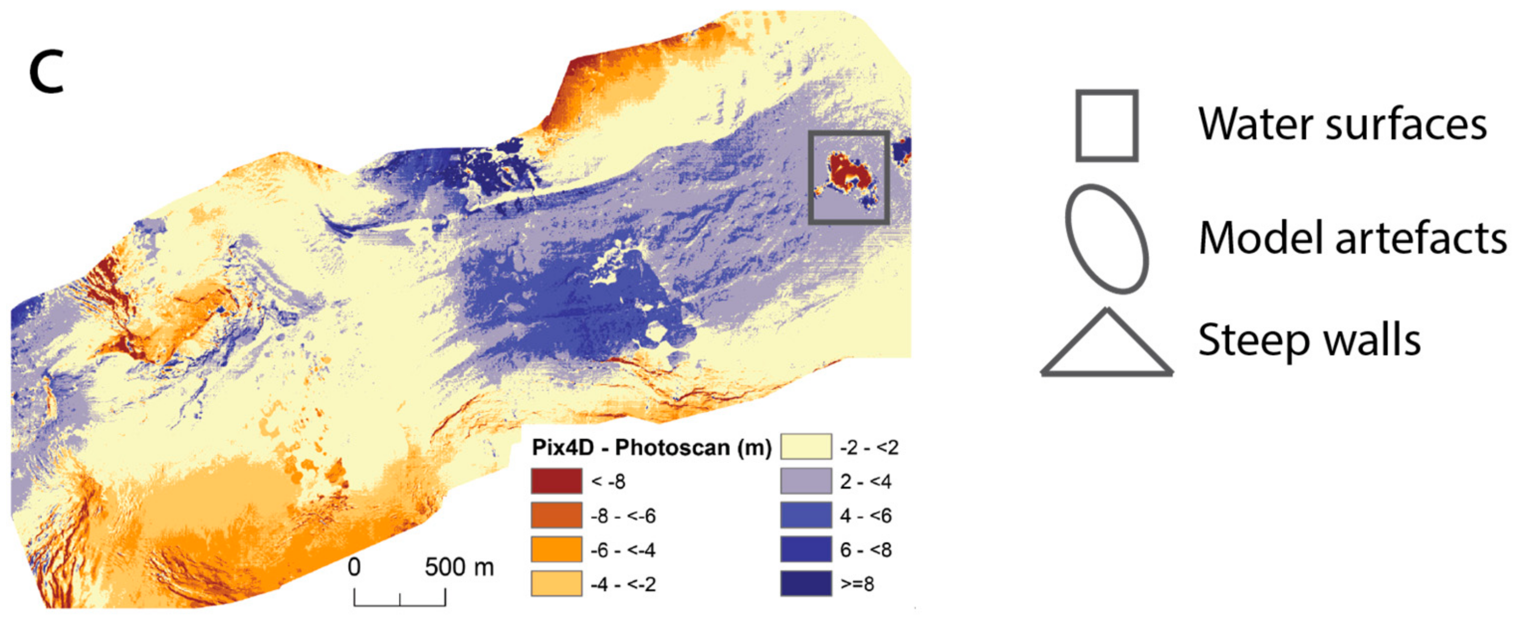
4.3. DTM Intercomparison
4.4. Orthophotos
4.5. Uncertainties
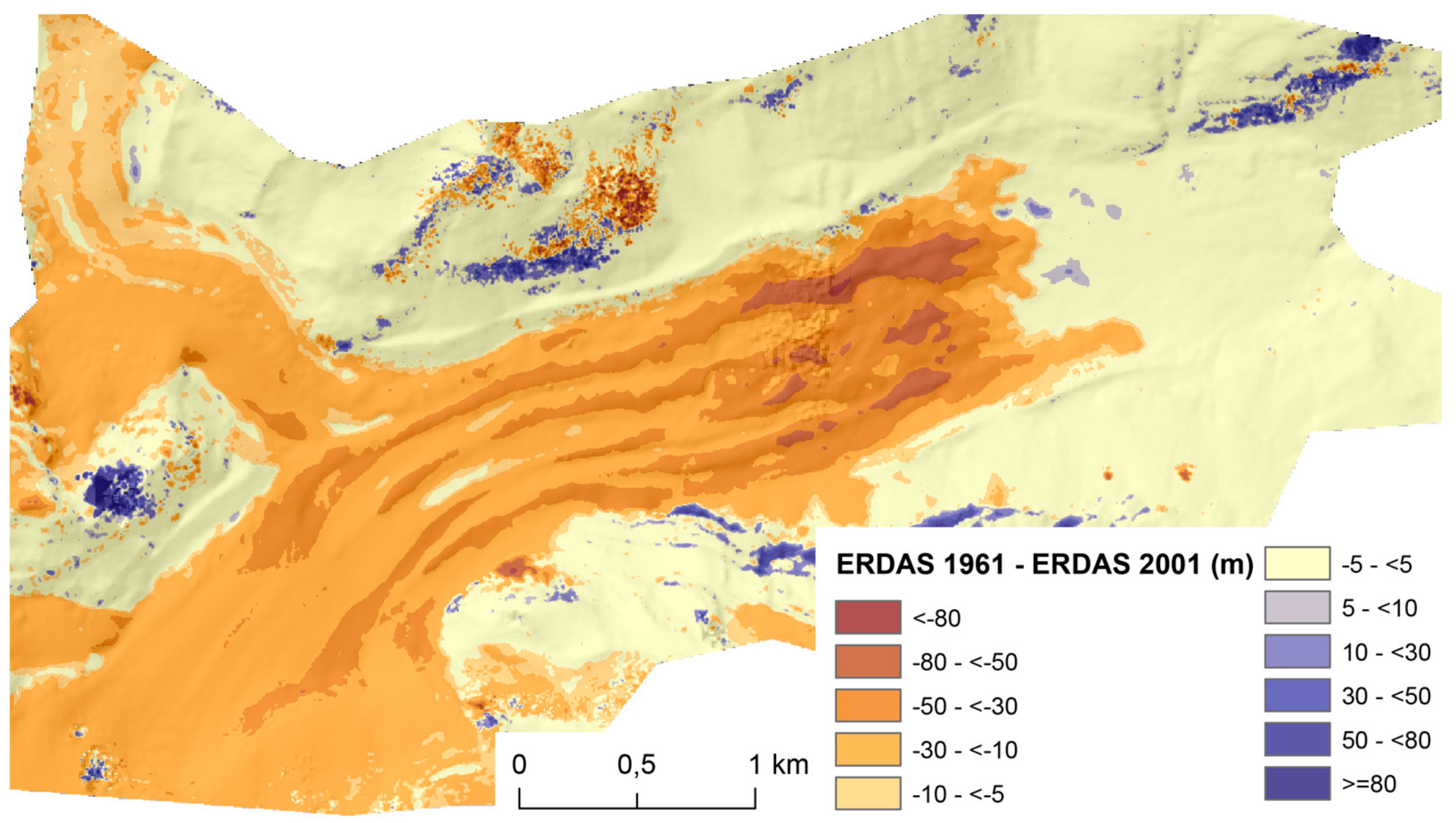
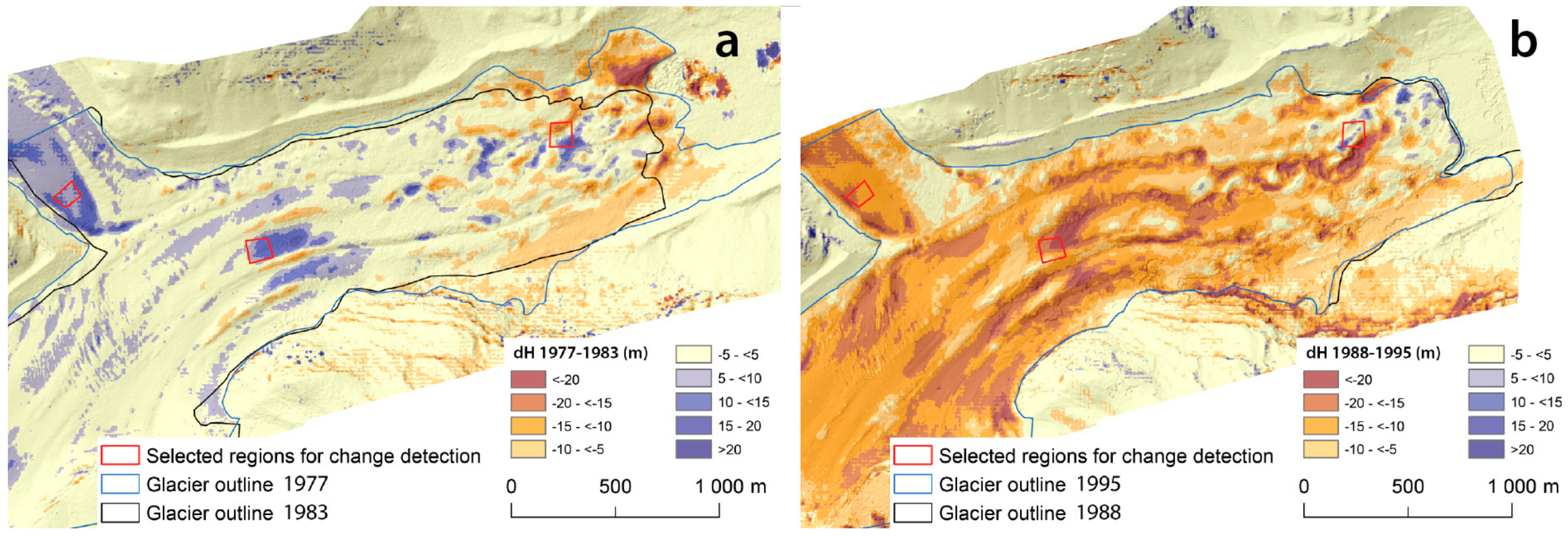
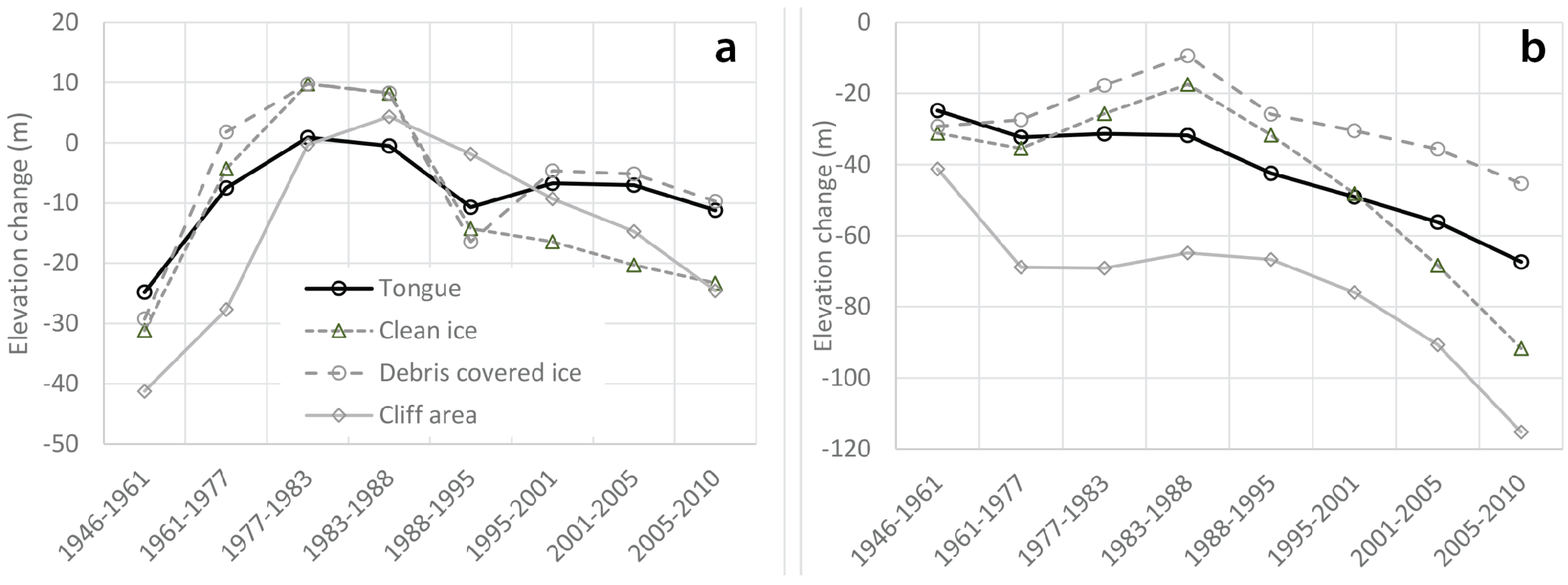
4.6. Glacier Evolution
5. Discussion
6. Conclusions
Acknowledgments
Author Contributions
Conflicts of Interest
References
- Smith, M.W.; Carrivick, J.L.; Quincey, D.J. Structure from motion photogrammetry in physical geography. Progress Phys. Geogr. 2016, 40, 247–275. [Google Scholar] [CrossRef]
- Eltner, A.; Kaiser, A.; Castillo, C.; Rock, G.; Neugirg, F.; Abellán, A. Image-based surface reconstruction in geomorphometry – merits, limits and developments. Earth Surf. Dynam. 2016, 4, 359–389. [Google Scholar] [CrossRef]
- Bakker, M.; Lane, S.N. Archival photogrammetric analysis of river-floodplain systems using Structure from Motion (SfM) methods. Earth Surf. Process. Landf. 2016, 28, 96. [Google Scholar] [CrossRef]
- Westoby, M.J.; Brasington, J.; Glasser, N.F.; Hambrey, M.J.; Reynolds, J.M. ‘Structure-from-Motion’ Photogrammetry: A low-cost, effective tool for geoscience applications. Geomorphology 2012, 179, 300–314. [Google Scholar] [CrossRef]
- Kraaijenbrink, P.; Shea, J.M.; Pellicciotti, F.; Jong, S.d.; Immerzeel, W.W. Object-based analysis of unmanned aerial vehicle imagery to map and characterise surface features on a debris-covered glacier. Remote Sens. Environ. 2016, 186, 581–595. [Google Scholar] [CrossRef]
- Rippin, D.M.; Pomfret, A.; King, N. High resolution mapping of supra-glacial drainage pathways reveals link between micro-channel drainage density, surface roughness and surface reflectance. Earth Surf. Process. Landf. 2015, 40, 1279–1290. [Google Scholar] [CrossRef]
- Kääb, A. Remote Sensing of Mountain Glaciers and Permafrost Creep. Habilitation; Geographisches Institut der Universität Zürich: Zürich, Switzerland, 2005. [Google Scholar]
- Bamber, J.L.; Rivera, A. A review of remote sensing methods for glacier mass balance determination. Glob. Planet. Chang. 2007, 59, 138–148. [Google Scholar] [CrossRef]
- Krimmel, R.M. Analysis of Difference Between Direct and Geodetic Mass Balance Measurements at South Cascade Glacier, Washington. Geogr. Ann. A 1999, 81, 653–658. [Google Scholar] [CrossRef]
- Bolstad, P.V.; Stowe, T. An Evaluation of DEM Accuracy: Elevation, Slope, and Aspect. Photogramm. Eng. Remote Sens. 1994, 60, 1327–1332. [Google Scholar]
- Pulighe, G.; Fava, F. DEM extraction from archive aerial photos: Accuracy assessment in areas of complex topography. Eur. J. Remote Sens. 2017, 46, 363–378. [Google Scholar] [CrossRef]
- Micheletti, N.; Lane, S.N.; Chandler, J.H. Application of archival aerial photogrammetry to quantify climate forcing of alpine landscapes. Photogram. Rec. 2015, 30, 143–165. [Google Scholar] [CrossRef]
- Glaciological reports (1881–2017). The Swiss Glaciers 1880–2015; Yearbooks of the Cryospheric Commission of the Swiss Academy of Sciences (SCNAT); VAW/ETH: Zurich, Switzerland, 2017.
- Zunino, L.; Ribeiro, H.V. Discriminating image textures with the multiscale two-dimensional complexity-entropy causality plane. Chaos Solitons Fractals 2016, 91, 679–688. [Google Scholar] [CrossRef]
- Federal Office of Topography swisstopo. swissALTI3D - Das hoch aufgelöste Terrainmodell der Schweiz. Available online: https://shop.swisstopo.admin.ch/de/products/height_models/alti3D (accessed on 3 May 2017).
- Federal Office of Topography swisstopo. Swissimage – Das digitale Farborthophotomosaik der Schweiz. Available online: https://shop.swisstopo.admin.ch/de/products/images/ortho_images/SWISSIMAGE (accessed on 18 May 2017).
- Hexagon Geospatial. ERDAS Imagine Photogrammetry; Hexagon Geospatial: Norcross, GA, USA, 2015. [Google Scholar]
- Kraus, K. Photogrammetrie, Bd 1; DE GRUYTER: Berlin, Germany, 2004. [Google Scholar]
- Grün, A.W.; Baltsavias, E.P. Geometrically constrained multiphoto matching. Photogramm. Eng. Remote Sens. 1988, 54, 633–641. [Google Scholar]
- Agisoft. PhotoScan, 2016.
- Javernick, L.; Brasington, J.; Caruso, B. Modeling the topography of shallow braided rivers using Structure-from-Motion photogrammetry. Geomorphology 2014, 213, 166–182. [Google Scholar] [CrossRef]
- Mertes, J.R.; Gulley, J.D.; Benn, D.I.; Thompson, S.S.; Nicholson, L.I. Using structure-from-motion to create glacier DEMs and orthoimagery from historical terrestrial and oblique aerial imagery. Earth Surf. Process. Landf. 2017, 54, 105. [Google Scholar] [CrossRef]
- Pix4D. Pix4Dmapper pro, 2016.
- Eltner, A.; Schneider, D. Analysis of Different Methods for 3D Reconstruction of Natural Surfaces from Parallel-Axes UAV Images. Photogram. Rec. 2015, 30, 279–299. [Google Scholar] [CrossRef]
- Lowe, D.G. Distinctive Image Features from Scale-Invariant Keypoints. Int. J. Comput. Vis. 2004, 60, 91–110. [Google Scholar] [CrossRef]
- Furukawa, Y.; Ponce, J. Accurate, dense, and robust multiview stereopsis. Trans. Pattern Anal. Mach. Intell. 2010, 32, 1362–1376. [Google Scholar] [CrossRef] [PubMed]
- Seitz, S.M.; Curless, B.; Diebel, J.; Scharstein, D.; Szeliski, R. A Comparison and Evaluation of Multi-View Stereo Reconstruction Algorithms. In 2006 IEEE Computer Society Conference on Computer Vision and Pattern Recognition—Volume 1 (CVPR’06), New York, NY, USA, 17–22 June 2006; IEEE: Hoboken, NJ, USA, 2006; pp. 519–528. [Google Scholar]
- Dandois, J.P.; Ellis, E.C. Remote Sensing of Vegetation Structure Using Computer Vision. Remote Sens. 2010, 2, 1157–1176. [Google Scholar] [CrossRef]
- Nuth, C.; Kääb, A. Co-registration and bias corrections of satellite elevation data sets for quantifying glacier thickness change. Cryosphere 2011, 5, 271–290. [Google Scholar] [CrossRef]
- Bolch, T.; Buchroithner, M.; Pieczonka, T.; Kunert, A. Planimetric and volumetric glacier changes in the Khumbu Himal, Nepal, since 1962 using Corona, Landsat TM and ASTER data. J. Glac. 2008, 54, 592–600. [Google Scholar] [CrossRef]
- Pieczonka, T.; Bolch, T.; Junfeng, W.; Shiyin, L. Heterogeneous mass loss of glaciers in the Aksu-Tarim Catchment (Central Tien Shan) revealed by 1976 KH-9 Hexagon and 2009 SPOT-5 stereo imagery. Remote Sens. Environ. 2013, 130, 233–244. [Google Scholar] [CrossRef]
- Smith, M.W.; Vericat, D. From experimental plots to experimental landscapes: Topography, erosion and deposition in sub-humid badlands from Structure-from-Motion photogrammetry. Earth Surf. Process. Landf. 2015, 40, 1656–1671. [Google Scholar] [CrossRef]
- Zemp, M.; Thibert, E.; Huss, M.; Stumm, D.; Rolstad Denby, C.; Nuth, C.; Nussbaumer, S.U.; Moholdt, G.; Mercer, A.; Mayer, C.; et al. Reanalysing glacier mass balance measurement series. Cryosphere 2013, 7, 1227–1245. [Google Scholar] [CrossRef]
- Zemp, M.; Paul, F.; Hoelzle, M.; Haeberli, W. Glacier Fluctuations in the European Alps, 1850–2000. In Darkening Peaks: Glacier Retreat, Science, and Society; Orlove, B.S., Wiegandt, E., Luckman, B.H., Eds.; University of California Press: Berkeley, CA, USA; London, UK, 2008; pp. 152–167. [Google Scholar]
- Gut, D.; Hohle, J. High Altitude Photography. Aspects and Results. Photogramm. Eng. Remote Sens. 1977, 43, 1245–1255. [Google Scholar]
- Shahbazi, M.; Sohn, G.; Théau, J.; Menard, P. Development and Evaluation of a UAV-Photogrammetry System for Precise 3D Environmental Modeling. Sensors 2015, 15, 27493–27524. [Google Scholar] [CrossRef] [PubMed]
- Rosnell, T.; Honkavaara, E. Point cloud generation from aerial image data acquired by a quadrocopter type micro unmanned aerial vehicle and a digital still camera. Sensors 2012, 12, 453–480. [Google Scholar] [CrossRef] [PubMed]
- Gindraux, S.; Boesch, R.; Farinotti, D. Accuracy Assessment of Digital Surface Models from Unmanned Aerial Vehicles’ Imagery on Glaciers. Remote Sens. 2017, 9, 186. [Google Scholar] [CrossRef]
- Immerzeel, W.W.; Kraaijenbrink, P.; Shea, J.M.; Shrestha, A.B.; Pellicciotti, F.; Bierkens, M.; de Jong, S.M. High-resolution monitoring of Himalayan glacier dynamics using unmanned aerial vehicles. Remote Sens. Environ. 2014, 150, 93–103. [Google Scholar] [CrossRef]
- Tonkin, T.; Midgley, N. Ground-Control Networks for Image Based Surface Reconstruction: An Investigation of Optimum Survey Designs Using UAV Derived Imagery and Structure-from-Motion Photogrammetry. Remote Sens. 2016, 8, 786. [Google Scholar] [CrossRef]
- Shao, Z.; Yang, N.; Xiao, X.; Zhang, L.; Peng, Z. A Multi-View Dense Point Cloud Generation Algorithm Based on Low-Altitude Remote Sensing Images. Remote Sens. 2016, 8, 381. [Google Scholar] [CrossRef]
- Ryan, J.C.; Hubbard, A.L.; Box, J.E.; Todd, J.; Christoffersen, P.; Carr, J.R.; Holt, T.O.; Snooke, N. UAV photogrammetry and structure from motion to assess calving dynamics at Store Glacier, a large outlet draining the Greenland ice sheet. Cryosphere 2015, 9, 1–11. [Google Scholar] [CrossRef]
- Piermattei, L.; Carturan, L.; de Blasi, F.; Tarolli, P.; Dalla Fontana, G.; Vettore, A.; Pfeifer, N. Suitability of ground-based SfM–MVS for monitoring glacial and periglacial processes. Earth Surf. Dynam. 2016, 4, 425–443. [Google Scholar] [CrossRef]


| Date | No. Images | Scale (ca.) | Flying Height | % Overlap Across/Along Track | Image Type | Texture (Shannon) | Image Size (cm) |
|---|---|---|---|---|---|---|---|
| 2 August 1946 | 7 | 50,000 | 8250 | 60/50 | BW | 4.82 | 23 × 23 |
| 18 August 1961 | 6 | 24,000 | 5100 | -/80 | BW | 4.91 | 18 × 18 |
| 14 September 1977 | 14 | 11,000 | 4100 | -/80 | BW | 4.76 | 23 × 23 |
| 8 September 1977 | 6 | 22,000 | 6200 | 20/80 | BW | 5.06 | 23 × 23 |
| 15 August 1983 | 11 | 11,000 | 4100 | -/80 | BW | 5.05 | 23 × 23 |
| 7 September 1988 | 29 | 22,000 | 6400 | 30/80 | BW | 5.06 | 23 × 23 |
| 12 October 1995 | 10 | 11,000 | 4200 | -/80 | BW | 5.18 | 23 × 23 |
| 29.8.2001 | 8 | 25,000 | 6400 | 30/70 | BW | 4.92 | 23 × 23 |
| 17.8.2005 | 4 | 25,000 | 6400 | -/70 | RGB | 5.16 | 23 × 23 |
| DTM Date | No. Images Total | Software | No. Images Used | DEM Reso-Lution (m) | RMSE (m) | No. GCPs | No. Tie Points |
|---|---|---|---|---|---|---|---|
| 2 August 1946 | 7 | ERDAS | 0 | ||||
| PhotoScan | 7 | 8 | 4.88 | 24 | 3476 | ||
| P4Dmapper | 0 | ||||||
| 18 August 1961 | 6 | ERDAS | 6 | 5 | 1.81 | 16 | 132 |
| PhotoScan | 6 | 3 | 3.18 | 8 | 19,373 | ||
| P4Dmapper | 6 | 2 | 0.45 | 10 | 47,613 | ||
| 14 September 1977 | 14 | ERDAS | 9 | 4 | 2.55 | 14 | 259 |
| PhotoScan | 13 | 4 | 0.41 | 18 | 32,447 | ||
| P4Dmapper | 14 | 1 | 1.14 | 17 | 118,495 | ||
| 8 September 1977 | 6 | ERDAS | 6 | 5 | 0.31 | 9 | 241 |
| PhotoScan | 6 | 3 | 0.80 | 11 | 19,679 | ||
| P4Dmapper | 6 | 5 | 0.35 | 10 | 59,637 | ||
| 15 August 1983 | 11 | ERDAS | 11 | 5 | 2.06 | 27 | 145 |
| PhotoScan | 11 | 3 | 0.25 | 16 | 16,091 | ||
| P4Dmapper | 11 | 2 | 1.64 | 13 | 133,748 | ||
| 7 September 1988 | 29 | ERDAS | 16 | 10 | 2.27 | 30 | 280 |
| PhotoScan | 28 | 5 | 1.68 | 25 | 82,794 | ||
| P4Dmapper | 21 | 5 | 5.05 | 21 | 236,311 | ||
| 12 October 1995 | 10 | ERDAS | 0 | ||||
| PhotoScan | 10 | 3 | 0.44 | 16 | 32,173 | ||
| P4Dmapper | 10 | 1 | 0.35 | 12 | 128,816 | ||
| 29 August 2001 | 8 | ERDAS | 8 | 5 | 1.05 | 23 | 127 |
| PhotoScan | 8 | 2 | 3.61 | 28 | 24,931 | ||
| P4Dmapper | 8 | 1 | 2.17 | 21 | 52,309 | ||
| 17 August 2005 | 4 | ERDAS | 4 | 2 | 1.87 | 21 | 70 |
| PhotoScan | 4 | 2 | 0.96 | 21 | 11,810 | ||
| P4Dmapper | 0 |
| DTM Date | ERDAS | Agisoft | Pix4D | ||||||
|---|---|---|---|---|---|---|---|---|---|
| Mean (m) | Std (m) | Range (m) | Mean | Std | Range | Mean | Std | Range | |
| 2 August 1946 | - | - | - | 3.10 | 5.00 | 59.00 | - | - | - |
| 18 August 1961 | −0.10 | 1.20 | 27.00 | −2.50 | 4.40 | 45.00 | 0.30 | 1.00 | 29.00 |
| 14 September 1977 | −1.00 | 3.90 | 196.40 | −1.00 | 1.60 | 25.30 | 0.43 | 1.00 | 22.30 |
| 8 September 1977 | −0.01 | 1.69 | 43.20 | −0.01 | 1.32 | 76.78 | 0.01 | 1.51 | 52.50 |
| 15 August 1983 | 0.08 | 1.42 | 43.70 | −0.26 | 1.65 | 30.20 | 0.65 | 1.78 | 47.90 |
| 7 September 1988 | −2.50 | 5.55 | 150.30 | 0.00 | 1.90 | 35.00 | 0.78 | 1.19 | 30.70 |
| 12 October 1995 | - | - | - | −0.42 | 3.33 | 35.60 | 0.10 | 0.77 | 24.00 |
| 29 August 2001 | 0.43 | 1.53 | 62.90 | 0.20 | 1.39 | 37.90 | −0.18 | 1.85 | 91.50 |
| 17 August 2005 | 0.37 | 0.88 | 35.67 | 0.60 | 1.02 | 43.56 | - | - | - |
| Average | −0.39 | 2.31 | 79.88 | −0.03 | 2.40 | 43.15 | 0.30 | 1.30 | 42.56 |
| DTM Date | ERDAS | PhotoScan | Pix4Dmapper | Max. Difference | ||||
|---|---|---|---|---|---|---|---|---|
| Mean (m) | Std (m) | Mean | Std | Mean | Std | Diff. (m) | Diff. (%) | |
| 2 August 1946 | - | - | 42.9 | 27.7 | - | - | - | - |
| 18 August 1961 | 38.7 | 16.9 | 27.8 | 20.53 | 39.2 | 16.9 | 11.4 | 29.1 |
| 14 Septembre 1977 | 33 | 14.1 | 34.3 | 13.7 | 34.5 | 14.1 | 1.5 | 4.3 |
| 8 Septembre 1977 | 26.6 | 14.4 | 26.4 | 14 | 27.7 | 15.1 | 1.3 | 4.7 |
| 15 August 1983 | 34.5 | 14.9 | 33.5 | 14.5 | 33.8 | 14.6 | 1 | 3.0 |
| 7 Septembre 1988 | 15.2 | 37.6 | 19 | 15.3 | 20.7 | 16.8 | 5.5 | 26.6 |
| 12 Octobre 1995 | - | - | 23.7 | 12 | 21.3 | 12 | 2.4 | 11.3 |
| 29 August 2001 | 11.9 | 9.1 | 12.7 | 8.8 | 13.2 | 11.4 | 1.3 | 9.8 |
| 17 August 2005 | 7.8 | 6.7 | 8.6 | 5.8 | - | - | 0.8 | 10.3 |
| Total all | 159.9 | 153.7 | 169.1 | 15.4 | 9.6 | |||
| Total selected | 106 | 106.9 | 109.2 | 3.2 | 3.0 | |||
© 2017 by the authors. Licensee MDPI, Basel, Switzerland. This article is an open access article distributed under the terms and conditions of the Creative Commons Attribution (CC BY) license (http://creativecommons.org/licenses/by/4.0/).
Share and Cite
Mölg, N.; Bolch, T. Structure-from-Motion Using Historical Aerial Images to Analyse Changes in Glacier Surface Elevation. Remote Sens. 2017, 9, 1021. https://doi.org/10.3390/rs9101021
Mölg N, Bolch T. Structure-from-Motion Using Historical Aerial Images to Analyse Changes in Glacier Surface Elevation. Remote Sensing. 2017; 9(10):1021. https://doi.org/10.3390/rs9101021
Chicago/Turabian StyleMölg, Nico, and Tobias Bolch. 2017. "Structure-from-Motion Using Historical Aerial Images to Analyse Changes in Glacier Surface Elevation" Remote Sensing 9, no. 10: 1021. https://doi.org/10.3390/rs9101021
APA StyleMölg, N., & Bolch, T. (2017). Structure-from-Motion Using Historical Aerial Images to Analyse Changes in Glacier Surface Elevation. Remote Sensing, 9(10), 1021. https://doi.org/10.3390/rs9101021