Hierarchical Terrain Classification Based on Multilayer Bayesian Network and Conditional Random Field

Abstract

This paper presents a hierarchical classification approach for Synthetic Aperture Radar (SAR) images. The Conditional Random Field (CRF) and Bayesian Network (BN) are employed to incorporate prior knowledge into this approach for facilitating SAR image classification. (1) A multilayer region pyramid is constructed based on multiscale oversegmentation, and then, CRF is used to model the spatial relationships among those extracted regions within each layer of the region pyramid; the boundary prior knowledge is exploited and integrated into the CRF model as a strengthened constraint to improve classification performance near the boundaries. (2) Multilayer BN is applied to establish the causal connections between adjacent layers of the constructed region pyramid, where the classification probabilities of those sub-regions in the lower layer, conditioned on their parents’ regions in the upper layer, are used as adjacent links. More contextual information is taken into account in this framework, which is a benefit to the performance improvement. Several experiments are conducted on real ESAR and TerraSAR data, and the results show that the proposed method achieves better classification accuracy.

1. Introduction

1.1. SAR Images Classification

Synthetic Aperture Radar (SAR) provides two-dimensional images independent from weather, daylight and cloud coverage conditions and has various applications, such as mapping, urban planning, disaster prevention [1], etc. Among these applications, terrain classification is one of the extremely active research interests. SAR images classification is a task to recognize objects by computing similarity and discrimination between them relying on the extracted features. An increasing number of papers specific to this topic have appeared over the last three decades; these proposed methods can be roughly cast into three categories: polarimetric target decomposition, feature extraction and model construction.

The polarimetric target decomposition method has been widely used in SAR image classification; the general idea behind this method is to represent the average backscattering as the sum of independent components. Two theories can be distinguished, namely coherent and incoherent decomposition. For the coherent decomposition, it aims to describe the scattering matrix as a combination of scattering responses. Since the polarization information is usually partially polarized, alternatively, the incoherent decomposition is used to express the target average matrix as the sum of the single scattering matrix; this approach provides a simplified way to extract geographical features. Over the years, a large number of associated methods have been proposed. The concept of target decomposition was first put forward by Huynen [2] for the analysis of scattering distribution in 1970. Pauli decomposition [3] was introduced by Cloude to decompose the polarization scattering matrix into four components. In 1990, Krogager [4] decomposed the complex symmetric scattering matrix into three components. In 1997, Cloude et al. proposed the $H/\alpha$ decomposition. After that, the target decomposition combining model was put forward, e.g., the three-component scattering model proposed by Freeman et al. [5]. In 2005, Yamaguchi [6] presented the four-component scattering model based on single reflection, secondary reflection and skew scattering. In 2007, Touzi [7] put forward incoherent decomposition, which is rotation invariant and is based on the coherent scattering model. In recent years, several new methods have been developed, such as three-component decomposition based on models [8] and the four-component decomposition model with extended scatterers [9].

Feature extraction has also received much attention. The most straightforward approach is to regard the scattering coefficient or the coherence/incoherence matrix as the underlying image features. Besides polarimetric features, texture has been proven as an efficient feature for image classification [10], such as the gray-level co-occurrence matrix [11], the wavelet with statistic textures [12], discrete wavelet transform [13], the semi-variance graph [14], etc. In 2011, Dai [15] put forward a multi-level local histogram descriptor, which is robust to speckle noise. It captures both local and global information and has been proven superior to the gray-level co-occurrence matrix and Gabor wavelet. In recent years, colorization for the SAR image has been developed. For instance, Deng et al. [16] proposed a method to visualize the SAR image based on the scattering mechanism. Tumer et al. [17] used the elliptic icon to express the data and to integrate the polarization characteristics into contextual information. Uhlmann et al. [18] employ various visible color descriptors to represent SAR images and then perform supervised classification. In [19,20], Golparvar and Balali present the texton-based and non-parameter feature extraction methods for image segmentation, which are innovative and can also be considered for SAR images.

Though much progress has been developed in SAR images classification, there are still some problems waiting to be resoled, especially for those images with complex structure information. For example, the extracted pixel-level features are often sensitive to the clutter. In this case, the information, provided by the image itself, fails to perform robust and effective classification. To overcome this limitation, several models have been proposed to incorporate additional prior knowledge to facilitate classification. For example, the Markov Random Field (MRF) [21], Conditional Random Field (CRF) [22] and Bayesian Network (BN) [23] are used to model prior knowledge for performance enhancement. MRF is widely used in SAR images’ interpretation; it captures the spatial interactions among neighborhoods as prior knowledge to guide classification. For instance, Elia [24] proposed a MRF model based on the regional and statistic texture; Voisin [25] put forward a multilayer MRF model based on texture information. However, with only local potential relationships considered in MRF, the connections among all observation data are ignored. As an extension of MRF, CRF is a discriminative model; it directly models the posterior probability of the sample labels. For example, Su et al. [26] construct a regional connected model to classify SAR images. Zhang et al. [27] integrate the class margin constraints into the CRF model to classify the spectral-based images. Ding [28] designs the unary potential, regional context potential and pairwise potential to improve the classification accuracy. As for the BN, which is a directed graphical model, it captures the causal relations among random variables. With the latent conditional independence, the joint probability can be factorized into several products of local conditional probabilities, which is a benefit to simplify the constructed model.

1.2. Motivation and Contributions

Although the multi-level CRF and BN model are adopted by those methods described above, it mainly focused on modeling either the spatial relationships or the causal dependencies alone. The hierarchical connections, namely the causal links between adjacent layers and the spatial relations within a sub-layer, are not combined together. The combination of a priori knowledge and image data itself plays an important role in performing robust and effective SAR image classification. To exploit this potential contextual information to improve classification accuracy, this paper presents a hierarchical classification framework based on the multilayer Bayesian network [29] and conditional random field.

The main contribution of this paper is that those causal dependencies between adjacent layers are incorporated into the proposed approach; what this means is that additional prior knowledge is exploited to improve classification accuracy. In SAR image classification, farmland, for example, is often far from urban areas, and therefore, the probability of a sub-region to be labeled as farmland, conditioned on its parents’ region, which is the urban area, is often small. Consequently, those existing dependencies between adjacent layers can be thought of as a priori information; the objective of the proposed method is to exploit this prior knowledge to improve the classification accuracy. Figure 1 illustrates a comparison between the proposed and the traditional methods. Compared with the traditional approach, the causalities between adjacent layers, as well as the spatial relationships within each layer are modeled by multilayer BN and CRF, respectively.

Figure 1. Comparison between the traditional and the proposed approaches. (a) Traditional single-layer model; (b) traditional multilayer model; CRF models the spatial relationships among those regions within each layer; (c) the proposed method combines CRF with BN into a unified framework, where BN captures the causal dependencies between adjacent layers, and therefore, more prior knowledge is exploited to guide classification.

The rest of this paper is organized as follows. Section 2 presents an overview of the proposed approach. Section 3 introduces the construction of a region pyramid by means of multiscale oversegmentation. Section 4 details how to build a semantic region pyramid by CRF and BN. Section 5 provides experimental results and the analysis. Finally, the conclusions are given in Section 7.

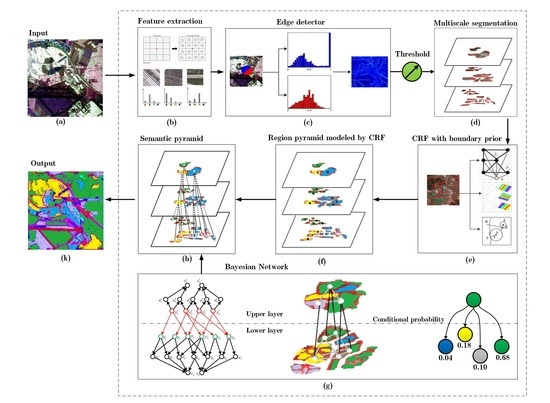
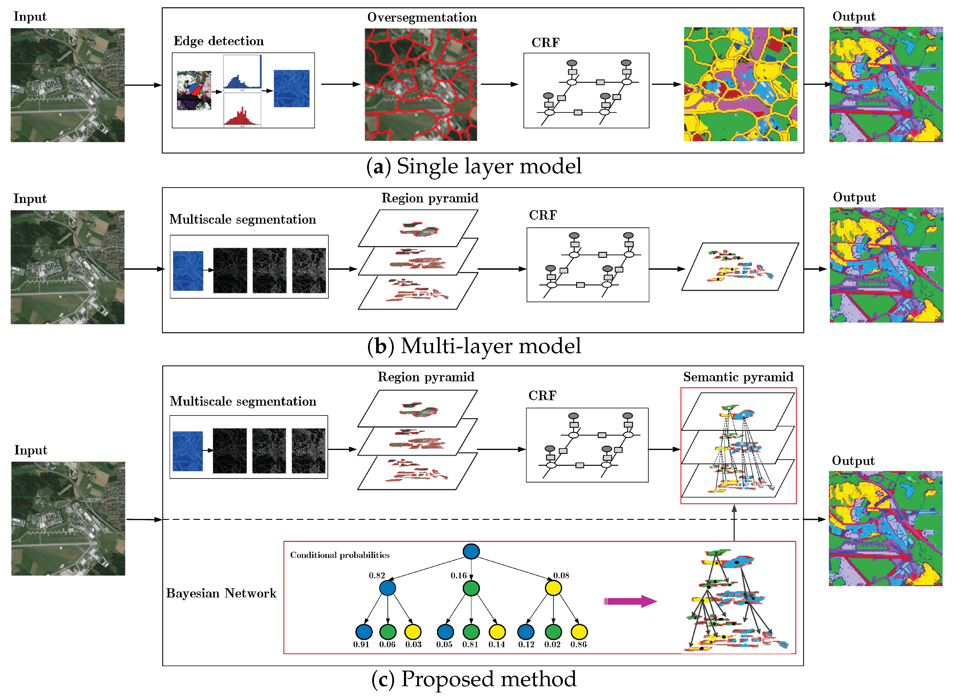
2. Overview of the Framework

The framework of the proposed classification method is illustrated in Figure 2. It mainly consists of three parts, i.e., the multiscale segmentation, the CRF and BN modeling.

Figure 2. Framework of the proposed method. (a) Input SAR image; (b) feature extraction, including intensity, polarization and texture features; (c) edge detection; (d) region pyramid construction based on multiscale segmentation; (e) conditional random field with boundary prior knowledge; (f) the region pyramid modeled by CRF; the spatial relationships are formed by CRF; (g) causal connections between adjacent layers are captured by the Bayesian network; (h) semantic pyramid based on the CRF and BN model; (i) classification output.

Multiscale segmentation: Given an input image, the multiscale segmentation is performed by adjusting an adaptive threshold, where the input image is partitioned into coarser and finer regions, namely superpixels. Then, a region pyramid is constructed by arranging the coarser oversegmentation on the top layer, whereas the finer one at the bottom layer. In this paper, a region pyramid with three layers is formed.

CRF modeling with boundary prior knowledge: With the above constructed region pyramid, the CRF is used to capture the spatial relationships among regions within each layer of the region pyramid. Moreover, the boundary prior knowledge is exploited and incorporated into the CRF model. With this additional prior information, it is equivalent to setting constraints to improve the classification accuracy near the boundaries.

Semantic pyramid construction by BN: Though the spatial relations among those regions within each layer can be effectively captured by the CRF model, the connections between adjacent layers are not explored and utilized. In order to establish these connections, BN is used to model the contextual information between adjacent layers of the region pyramid, and therefore, a semantic pyramid can be formed. Here, the BN models the causal relationships between those regions in the upper layer and its sub-regions in the lower layer. The causalities are referred to as the classification probabilities of those sub-regions conditioned on their parents’ regions, where the causalities are obtained from the statistical results of CRF labeling. In addition, the natural existing relationships among the regions, edges and vertices are also modeled in BN, where the edge is formed by two regions with different classes, and the vertex corresponds to the intersection of edges. In other words, more prior knowledge is integrated into the proposed classifying framework to enhance classification performance.

3. Multiscale Segmentation

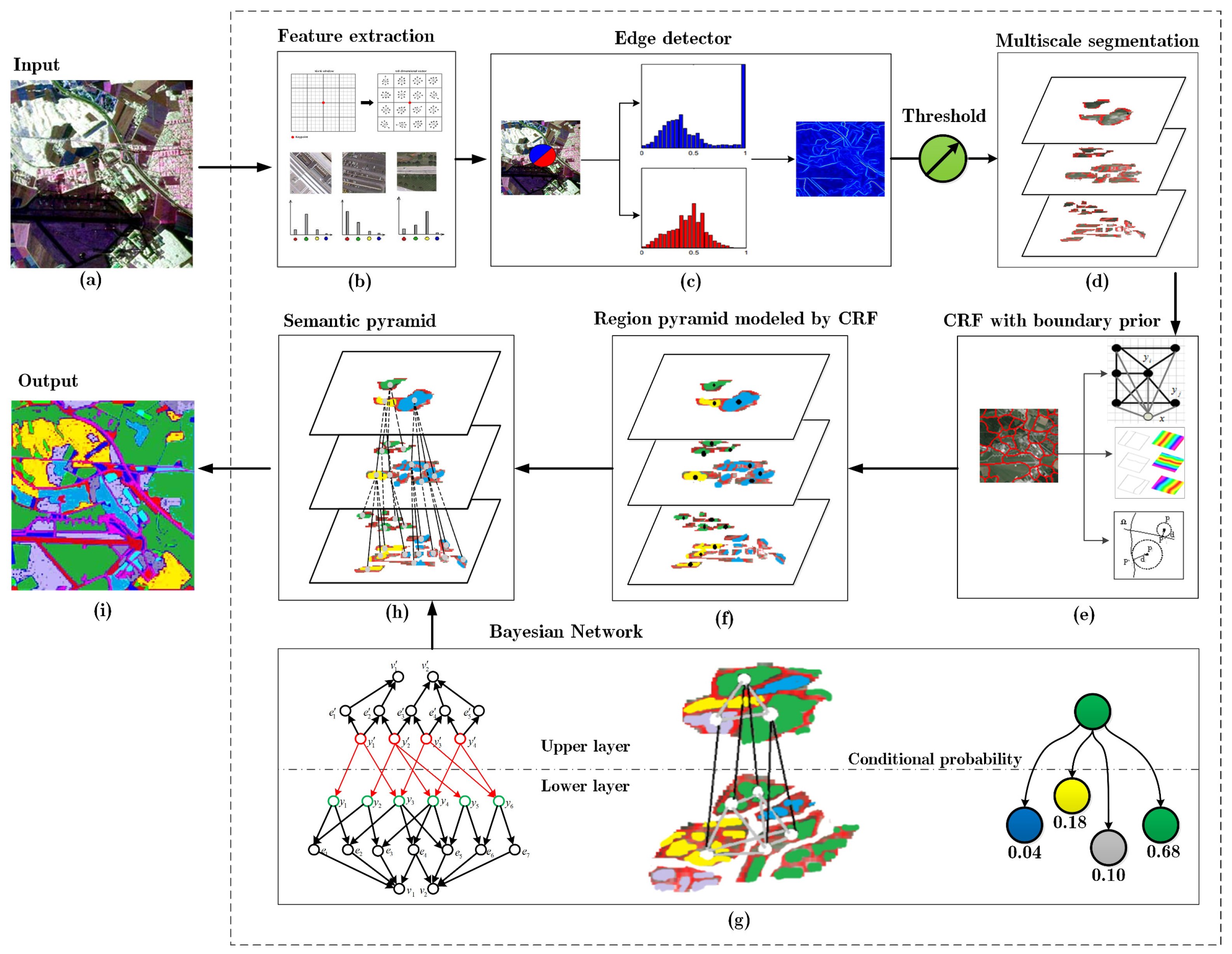
In this paper, we construct a region pyramid with three layers, where each layer contains the oversegmented regions of the input image. To construct such a region pyramid, edge detection is first performed, and then, those extracted edges are combined to form several closed regions. The last step is multiscale segmentation; the finer and coarser regions can be obtained by adjusting a threshold.

3.1. Edge Detection

Given an image I, in order to predict an edge with orientation θ at location $(x,y)$, the image is first transformed into three feature channels, including intensity, polarization and texture, then the gradients for these feature channels are calculated. Finally, an improved detector $gDet\left(x,y,\theta \right)$ is designed by combining those gradients for edge detection.

Intensity, polarization and texture gradients: An edge corresponds to the change between neighboring areas in an image, and the gradient describes this characteristic. In order to extract the gradient, a circular disc with radius σ is placed at location $(x,y)$; this disc splits the local region into two sub-regions g and h, and the orientation is defined by a diameter at angle θ. The magnitude of gradient $G(x,y,\theta )$ at $(x,y)$ is defined as the histograms’ chi-square distance between the two sub-regions, which is given by:

$$\begin{array}{c}\hfill \begin{array}{c}\hfill \parallel G(x,y,\theta )\parallel =\frac{1}{2}\sum _i\frac{{\left(g(i)-h(i)\right)}^2}{g(i)+h(i)}\end{array}\end{array}$$

(1)

where $g(i)$ and $h(i)$ denote the i-th element in the histograms of the sub-regions g and h, respectively. Here, three types of feature are extracted, i.e., multi-channel intensity, polarization and texture, and then, the gradient is calculated in each feature channel independently.

Multiscale linear combination: To detect the desired fine and coarse structure information, the gradient of each feature channel is computed at three scales: $[\sigma /2,\sigma ,2\sigma ]$. For the intensity, $\sigma =5$ pixels; as for polarization and texture, $\sigma =10$ pixels. Then, these extracted gradients are linearly combined together to form $mDet\left(x,y,\theta \right)$, which is defined as:

$$\begin{array}{c}\hfill \begin{array}{c}\hfill mDet\left(x,y,\theta \right)={\displaystyle \sum _s}{\displaystyle \sum _i}{\alpha }_{i,s}{G}_{i,\sigma \left(i,s\right)}\left(x,y,\theta \right)\end{array}\end{array}$$

(2)

where s and i denote the scale and feature channel; $G_{i,\sigma \left(i,s\right)}\left(x,y,\theta \right)$ is the gradient at location $(x,y)$ in channel i with a radius $\sigma (i,s)$ and orientation θ; $a_{i,s}$ represents the weight for each gradient. In this paper, eight orientations are sampled in interval $[0,\pi )$ with equal space, and the maximum $mDet\left(x,y\right)$ over orientations is defined as the boundary response at location $(x,y)$, which is given by:

$$\begin{array}{c}\hfill \begin{array}{c}\hfill mDet\left(x,y\right)=\underset{\theta }{max}\left\{mDet\left(x,y,\theta \right)\right\}\end{array}\end{array}$$

(3)

Curve and edge detection: Spectral clustering [30] is applied to image segmentation. A sparse symmetric incidence matrix W is constructed by the maximum of $mDet$; the elements of W measure the similarity between pixels. The normalized cuts algorithm is used to solve the standard feature vector; a descriptor with n-dimensions is extracted for each pixel, and the clustering algorithm, such as k-means, is employed to segment the image. In order to obtain the correct partition, a convolution step is concluded, where Gaussian-oriented derivative filters are used at multiple orientations. Therefore, the spectral boundary detector $sDet\left(x,y,\theta \right)$ is defined as:

$$\begin{array}{c}\hfill \begin{array}{c}\hfill sDet\left(x,y,\theta \right)={\displaystyle \sum _{k=1}^n}{\lambda }_k^{-\frac{1}{2}}{\nabla }_{\theta }{v}_k\left(x,y\right)\end{array}\end{array}$$

(4)

where ${\nabla }_{\theta }{v}_k\left(x,y\right)$ denotes the oriental signal and ${\lambda }_k$ is the k-th eigenvalue. Notice that $mDet$ carries edge information, while $sDet$ conveys the curve information in an image. In order to extract both the edge and curve information, a linear combination of $mDet$ and $sDet$ is constructed, and then, an improved detector $gDet$ is given by:

$$\begin{array}{c}\hfill \begin{array}{c}\hfill gDet\left(x,y,\theta \right)={\displaystyle \sum _s}{\displaystyle \sum _i}{\beta }_{i,s}{G}_{i,\sigma (i,s)}\left(x,y,\theta \right)+\omega ·sDet\left(x,y,\theta \right)\end{array}\end{array}$$

(5)

where ${\beta }_{i,s}$ and ω can be learned during the training procedure. For more details, please refer to the original paper [30].

3.2. Region Pyramid Construction

Here, the region pyramid contains three layers, where these layers, from top to bottom, correspond to the undersegmentations and oversegmentations of the initial image, respectively. In order to construct such a region pyramid, a multiscale segmentation process is required; the initial image is partitioned recursively by adjusting a threshold; and a set of fine and coarse segmentations, namely regions, can be produced and used to form the region pyramid.

The Oriented Watershed Transformation (OWT) [30] is first used to construct an initial segmentation; the output of OWT is the finest partition for the region pyramid. Then, a sequence of the Ultrametric Contour Map (UCM) [31] can be produced by adjusting the threshold, where the UCM describes the strength of the curve boundary, namely the probability of being a true contour. Consequently, the oversegmentations and undersegmentations can be obtained; Figure 3 shows an example of multiscale segmentation. Finally, the region pyramid can be constructed by arranging the coarsest UCM at the top layer, whereas the finest UCM at the bottom layer.

Figure 3. Multiscale segmentation under three different thresholds. (a) The input SAR image; (b–d) the segmentation results by adjusting the threshold k. The lower the threshold is set, the more sub-regions are detected.

4. Semantic Pyramid Construction by CRF and BN

With the region pyramid constructed above, prior knowledge is exploited to form a semantic pyramid. The prior knowledge consists of the spatial relationships among those regions within each sub-layers and the causal connections between adjacent layers, which are modeled by CRF and BN, respectively.

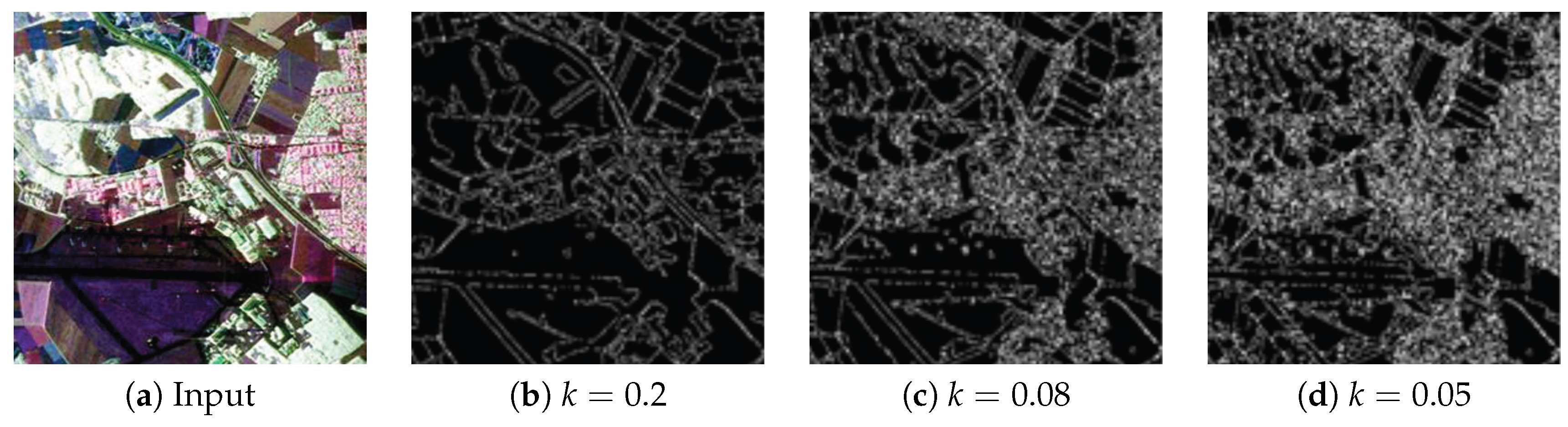
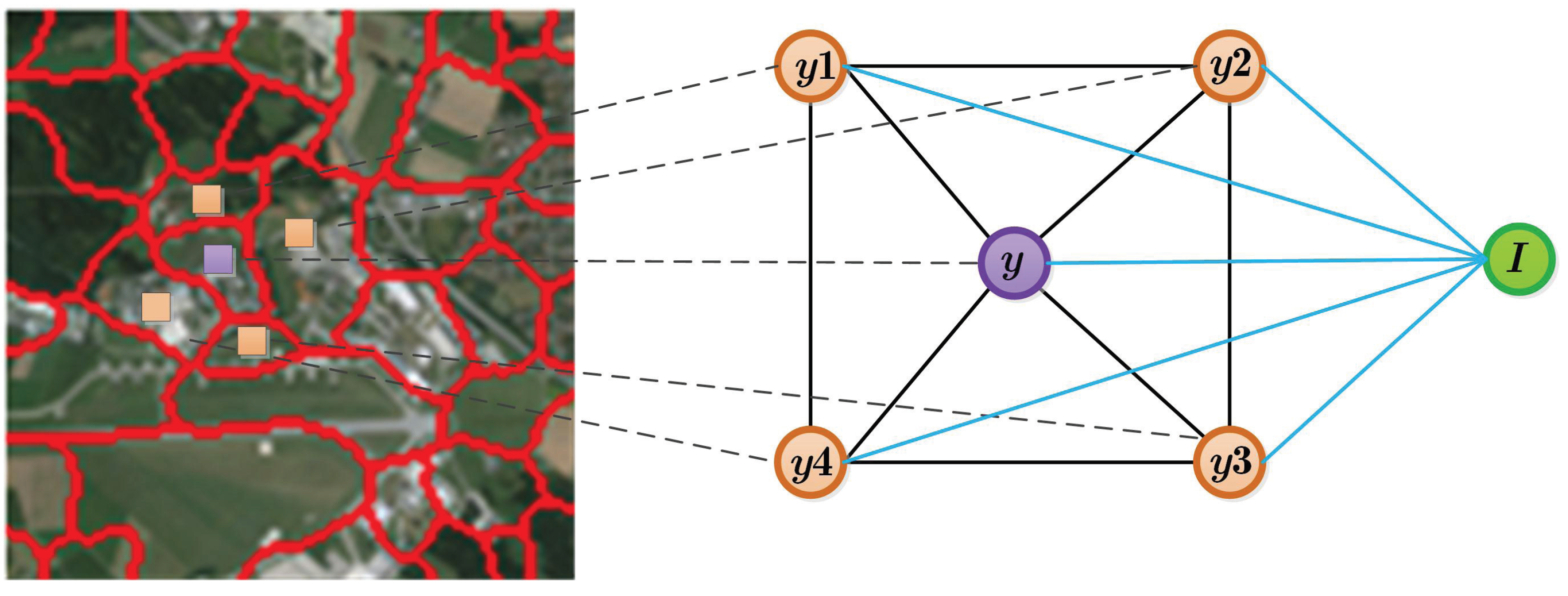
4.1. CRF with Boundary Prior Knowledge

CRF is a discriminative model, and it can effectively capture the spatial relationships among random variables. In this paper, the boundary prior knowledge is also considered and integrated into the CRF model to improve the classification accuracy of such regions near the boundary.

Standard CRF: As shown in Figure 4, the image is oversegmented into several regions, and CRF is used to model the spatial relationships among those regions; here, the regions correspond to the nodes in CRF. Given an image I, let x denote the observation data, namely the pixel, and y is the label to be assigned. Then, let $I=\{x_1,x_2,\cdots ,x_M\}$ represent image segmentation, where $x_i$ denotes the i-th oversegmentation, namely a superpixel (a collection of some pixels), $i\in S=\{1,2,\cdots ,M\}$. The posterior probability $P\left(y|\varphi \left(x\right)\right)$ is given by:

$$\begin{array}{c}\hfill \begin{array}{c}\hfill P\left(y|\varphi \left(x\right)\right)=\frac{1}{Z\left(x\right)}exp\left\{{\displaystyle \sum _{i\in S}}{A}_i\left(y_i,{\varphi }_i\left(x\right)\right)+\right.\left.{\displaystyle \sum _{i\in S}}{\displaystyle \sum _{j\in N_i}}{I}_{ij}\left(y_i,y_j,\mu \left({\varphi }_i\left(x\right),{\varphi }_j\left(x\right)\right)\right)\right\}\end{array}\end{array}$$

(6)

where j is a superpixel in the spatial neighborhood $N_i$ of i and $A_i$ and $I_{ij}$ denote the unary potential and pairwise potential, respectively. The feature function ${\varphi }_i\left(x\right)$ maps the i-th oversegmentation data $x_i$ to the feature space, and $\mu ({\varphi }_i(x),{\varphi }_j(x))$ is the feature vector of pairwise block $(i,j)$. $Z\left(x\right)$ is the partition function, which is defined as:

$$\begin{array}{c}\hfill \begin{array}{c}\hfill Z\left(x\right)={\displaystyle \sum _{y_i}}exp\left\{{\displaystyle \sum _{i\in S}}{A}_i\left(y_i,{\varphi }_i\left(x\right)\right)+{\displaystyle \sum _{i\in S}}{\displaystyle \sum _{j\in N_i}}{I}_{ij}\left(y_i,y_j,\mu \left({\varphi }_i\left(x\right),{\varphi }_j\left(x\right)\right)\right)\right\}\end{array}\end{array}$$

(7)

Figure 4. The spatial relationships are modeled by the conditional random field. The image is first partitioned into several regions, then the CRF is used to model the spatial relationships among those regions, where the node y represents a region, while x denotes the whole image.

CRF with boundary prior knowledge: During CRF inference, the pixels within a region are assigned to the same label since such a region is considered as a homogeneous block, and the adjacent regions are often labeled as different categories. However, those adjacent regions may be of the same label. To overcome this limitation, the boundary prior knowledge is incorporated into the CRF model as a constraint to improve the classification accuracy near the boundaries.

The boundary prior knowledge refers to the distance between the boundary and pixel or superpixel. If the label of the current pixel is the same as its neighborhoods, the greater the distance between the pixel and boundary, the weaker the relationship between them. Otherwise, this boundary prior information can be ignored. Here, the boundary is the strong response of the watershed transform algorithm. Given a curve Ω, the distance between pixel p and Ω is defined as the minimum Euclidean distance between p and the points on Ω, which is given by:

$$\begin{array}{c}\hfill \begin{array}{c}\hfill d=dist(p,\Omega )=dist(p,p^{\prime })=\sqrt{{(x_p-x_{p^{\prime }})}^2+{(y_p-y_{p^{\prime }})}^2}\end{array}\end{array}$$

(8)

where $p^{\prime }$ is the nearest point to p and $x_p$, $y_p$ and $x_p^{\prime }$, $y_p^{\prime }$ are the associated coordinates, respectively.

Based on the above definition, the boundary prior knowledge can be obtained from the labeled image, where the labeling procedure is implemented by CRF. In order to define the conditional probability with the boundary prior knowledge, let $\Omega =\{{\Omega }_1,\cdots ,{\Omega }_H\}$ denote the H nearest lines to pixel $p_i$; $R_h$ represents the h-th region; and $R_h$ contains the line ${\Omega }_h$, where $h=1,2,\cdots ,H$. Then, the conditional probability with boundary prior knowledge of $p_i$ labeled as c can be given by:

$$P_{BP}\left(c|p_i,\Omega ,c^{\prime }\right)=exp\left({\displaystyle \sum _{h=1}^H}\gamma ·t\left(c,p_i,R_h\right)·F\left(dis\left(p_i,{\Omega }_h\right)\right)\right)$$

(9)

where γ is the parameter for boundary prior knowledge and can be learned by the training process, $c^{\prime }$ denotes the original label by CRF and $t\left(c,p_i,R_j\right)$ and $F\left(dis\left(p_i,{\Omega }_j\right)\right)$ are defined as:

$$\left\{\begin{array}{c}F\left(dis\left(p_i,{\Omega }_j\right)\right)=\frac{1}{1+exp\left\{dist\left(p_i,{\Omega }_j\right)-\lambda \right\}}\hfill \\ t\left(c,p_i,R_j\right)=\left\{\begin{array}{cc}1,\hfill & \mathrm{if}{p}_i\in R_h\mathrm{and}c=max\left(c^{\prime },R_h\right)\hfill \\ 0,\hfill & \mathrm{otherwise}\hfill \end{array}\right.\hfill \end{array}\right.$$

(10)

where $F\left(dis\left(p_i,{\Omega }_j\right)\right)$ is the potential function, threshold λ is used to normalize the distance $dis\left(p_i,{\Omega }_j\right)$ within interval $(0,1)$ and $t\left(c,p_i,R_j\right)$ ensures $p_i$ to be labeled the same as its neighborhoods.

With the above definition, the Equation (6) can be re-written as:

$$\begin{array}{c}\hfill \begin{array}{c}\hfill \begin{array}{c}P(y_i|\varphi (x_i),\Omega ,c^{\prime })\propto P_{Pi}(y_i)·P_{Li}(\varphi (x_i)|y_i)·P_{BP}(y_i|\varphi (x_i),\Omega ,c^{\prime })\hfill \end{array}\end{array}\end{array}$$

(11)

where $P_{Pi}$ and $P_{Li}$ denote the prior and likelihood terms in Equation (6), respectively. The $P_{BP}(y_i|\varphi (x_i),\Omega ,c^{\prime })$ is given by:

$$P_{BP}\left(y_i|\varphi (x_i),\Omega ,c^{\prime }\right)={\displaystyle \sum _{p_i\in x_i}}{P}_{BP}\left(y_i|p_i,\Omega ,c^{\prime }\right)$$

(12)

where $x_i$ denotes a superpixel and $p_i$ is a pixel within $x_i$.

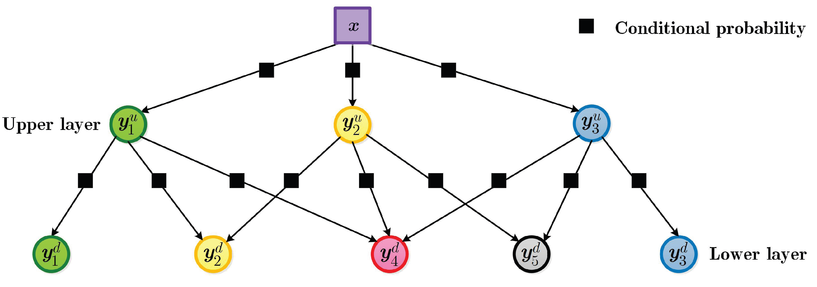
4.2. Multi-Layer Bayesian Network

The causal connections between adjacent layers are modeled by BN; these connections are referred to as the classification probabilities of the sub-regions in the lower layer conditioned on their parents’ regions in the upper layer. In addition, the causal dependencies among regions, edges and vertices are also taken into account and modeled by BN.

Causal connections between adjacent layers: As described in Section 2, the regions in the top layer can be further divided into several sub-regions in the lower layer by means of multiscale oversegmentation. Note that the labels to be assigned to those sub-regions do have some dependencies on their parents’ regions in the top layer. In terrain classification from SAR images, for example, the roads often intersect within the buildings and are far from the forests; the farmland is often far from the urban areas, and so on. These dependencies can be thought of as additional contextual knowledge to link the adjacent layers and can be exploited to improve classification accuracy.

The labeled probability of a sub-region conditioned on its parent region can be defined as the following conditional probability:

$$\begin{array}{c}\hfill \begin{array}{c}\hfill P\left(y^d=c_i|y^u=c_j\right)={\phi }_{ij}\end{array}\end{array}$$

(13)

where $y^d$ and $y^u$ denote the labels of the sub-region in the lower layer and its parent region in the upper layer, and the corresponding assigned labels are $c_i$ and $c_j$, respectively; ${\phi }_{ij}$ is the conditional probability. This conditional probability can be obtained from the statistical results of the CRF labeling. For SAR image classification, if there are N classes, a Conditional Probability Table (CPT) with $N\times N$ dimensions can be used to describe those causalities. Figure 5 illustrates the causal connections between adjacent layers, where the causalities are constructed by those classification probabilities of sub-regions in the lower layer conditioned on their parents’ regions in the upper layer.

Figure 5. The causal connections between adjacent layers are modeled by the Bayesian network. The input image x is first coarsely classified into labels $y_1^u,y_2^u,y_3^u$ in the upper layer, and then, those regions in the upper layer are finely labeled into $y_1^d,y_2^d,y_3^d,y_4^d,y_5^d$ in the lower layer, where the classification probabilities of the sub-regions in the lower layer, conditioned on their parents’ regions in the upper layer, are denoted by black squares.

Regions’, edges’ and vertices’ relationships: The relationships among regions, edges and vertices refers to such contextual knowledge, which has been extensively exploited by humans. The edge is formed by the intersection of regions with different labels; the vertex is from the intersections of edges. Figure 6 illustrates the causalities among regions, edges and vertices; edge $e_2$, for example, is formed by regions $y_3$ and $y_4$, and therefore, $y_3$ and $y_4$ are the parents nodes of $e_2$. These contexts can be modeled by conditional probabilities in BN.

Figure 6. The causalities among regions, edges and vertices. An edge is formed by the intersection of the regions with different labels, and these regions are the parent nodes of the edge. The vertex is formed by edges, and these associated edges are the parent nodes of the vertex.

The BN model constructed here is based on the oversegmentation edge graph; the edge graph consists of edges ${\left\{e_j\right\}}_{j=1}^m$ and vertices ${\left\{v_t\right\}}_{t=1}^l$, where m and l denote the numbers of edges and vertices. There are two states to be assigned to the edges and vertices, namely $true$ or $false$ represented by one and zero, respectively. BN models the causal relationships among the oversegmentation regions ${\left\{y_i\right\}}_{i=1}^n$, the edges ${\left\{e_j\right\}}_{j=1}^m$ and vertices ${\left\{v_t\right\}}_{t=1}^l$.

For an edge, it is formed by the intersection of two regions, which are defined as the edge’s parent nodes. Consequently, if the labels of the parent nodes are different, it is likely that there is a true boundary existing between the two regions, namely $e_j=1$. The conditional probability can be defined as:

$$P\left(e_j=1|pa\left(e_j\right)\right)=\left\{\begin{array}{cc}0.8\hfill & \mathrm{labels}\mathrm{of}\mathrm{parent}\mathrm{nodes}\mathrm{are}\mathrm{different},\hfill \\ 0.2\hfill & \mathrm{others}.\hfill \end{array}\right.$$

(14)

where $pa\left(e_j\right)$ denotes the parent node of edge $e_j$.

As for the vertex, its parent nodes are those intersecting edges. In this paper, a vertex is formed by at least three edges. Therefore, the conditional probability between the vertex and its parent nodes can be defined as:

$$P\left(v_t=1|pa\left(v_t\right)\right)=\left\{\begin{array}{cc}0.7\hfill & \mathrm{more}\mathrm{than}\mathrm{two}\mathrm{edge}\mathrm{nodes}\mathrm{are}\mathrm{true},\hfill \\ 0.3\hfill & \mathrm{others}.\hfill \end{array}\right.$$

(15)

where $pa\left(v_t\right)$ is the parent node of vertex $v_t$.

Let $\mathit{y}$, $\mathit{e}$ and $\mathit{v}$ represent all of the regions ${\left\{y_i\right\}}_i^n$, edges ${\left\{e_j\right\}}_j^m$ and ${\left\{v_t\right\}}_t^l$, respectively, then the image classification can be performed by inferring the optimal states ${\mathit{y}}^{*}$, ${\mathit{e}}^{*}$ and ${\mathit{v}}^{*}$:

$$\begin{array}{c}\hfill \begin{array}{c}\hfill {\mathit{y}}^{*},{\mathit{e}}^{*},{\mathit{v}}^{*}=arg\underset{\mathit{y},\mathit{e},\mathit{v}}{max}P\left(\mathit{y},\mathit{e},\mathit{v}\right)\end{array}\end{array}$$

(16)

where $P\left(\mathit{y},\mathit{e},\mathit{v}\right)$ is the joint probability. With the assumption of conditional independence in BN, the joint probability can be expressed as the product of local conditional probabilities, which is given by:

$$\begin{array}{c}\hfill \begin{array}{c}\hfill P\left(\mathit{y},\mathit{e},\mathit{v}\right)={\displaystyle \prod _{i=1}^n}P\left(y_i\right){\displaystyle \prod _{j=1}^m}P\left(e_j|pa\left(e_j\right)\right){\displaystyle \prod _{t=1}^l}P\left(v_t|pa\left(v_t\right)\right)\end{array}\end{array}$$

(17)

where $P\left(y_i\right)$ is the prior probability of regions. With the consideration of insufficient training samples in practice, here uniform distribution is used to model the prior probability. With the causal relationships of the adjacent layers modeled by multilayer BN, a semantic pyramid is built from the region pyramid constructed in Section 3. The joint probability of the multilayer BN is given by:

$$\begin{array}{cc}\hfill P\left(\mathit{y},\mathit{e},\mathit{v},\mathit{x}\right)=& \prod _{<u,d>\in {\rm Y}}{\displaystyle \prod _{i=1}^n}P\left(y_i^u\right){\displaystyle \prod _{j=1}^m}P\left(e_j^u|pa\left(e_j^u\right)\right){\displaystyle \prod _{t=1}^l}P\left(v_t^u|pa\left(v_t^u\right)\right)·\hfill \\ & {\displaystyle \prod _{i^{\prime }=1}^{n^{\prime }}}P\left(y_i^d\right){\displaystyle \prod _{j^{\prime }=1}^{m^{\prime }}}P\left(e_j^d|pa\left(e_j^d\right)\right){\displaystyle \prod _{t^{\prime }=1}^{l^{\prime }}}P\left(v_t^d|pa\left(v_t^d\right)\right)·P\left(y^d=c|y^u=c^{\prime }\right)\hfill \end{array}$$

(18)

where $<u,d>\in {\rm Y}$ denotes the combination of the adjacent layers; the numbers of classes, edges and vertices in the second layer of BN are represented by $n^{\prime }$, $m^{\prime }$ and $l^{\prime }$, respectively.

4.3. Unified Inference Model for CRF and BN

Since both CRF and BN are included to model prior knowledge, to perform a global inference, the Factor Graph (FG) is used to represent the CRF and BN in a unified framework. In FG, the global joint probability is described by a set of factorization, where the random variable node is represented by a circle and the factor node by a solid square; if and only if two variables are relevant, there exits a connection between them.

With the assumption of the global Markov property in FG, the joint probability of each layer in semantic pyramid $P\left(\mathit{y},\mathit{e},\mathit{v},\mathit{x}\right)$ can be factorized by:

$$P\left(\mathit{y},\mathit{e},\mathit{v},\mathit{x}\right)=P\left(\mathit{e},\mathit{v}|\mathit{y},\mathit{x}\right)P\left(\mathit{y},\mathit{x}\right)=P\left(\mathit{v}|\mathit{e}\right)P\left(\mathit{e}|\mathit{y}\right)P\left(\mathit{y}|\mathit{x}\right)P\left(\mathit{x}\right)$$

(19)

where $P\left(\mathit{v}|\mathit{e}\right)$ and $P\left(\mathit{e}|\mathit{y}\right)$ denote the causalities among edges, vertices and labels in BN, namely Equations (14) and (15), respectively; $P\left(\mathit{y}|\mathit{x}\right)$ represents Equation (6), and $P\left(\mathit{x}\right)$ is constant because $\mathit{x}$ is observed.

Note that the constructed semantic pyramid consists of a multilayer, where the causal connections between adjacent layers are modeled by BN, and therefore, the global joint probability $P\left(\mathit{y},\mathit{e},\mathit{v},\mathit{x}\right)$ can be expressed by:

$$\begin{array}{c}\hfill \begin{array}{c}\hfill P\left(\mathit{y},\mathit{e},\mathit{v},\mathit{x}\right)=\prod _{<u,d>\in {\rm Y}}{P}_u\left(\mathit{y},\mathit{e},\mathit{v},\mathit{x}\right)P_d\left(\mathit{y},\mathit{e},\mathit{v},\mathit{x}\right)P\left(y^d=c|y^u=c^{\prime }\right)\end{array}\end{array}$$

(20)

where $P_u\left(\mathit{y},\mathit{e},\mathit{v},\mathit{x}\right)$ and $P_d\left(\mathit{y},\mathit{e},\mathit{v},\mathit{x}\right)$ denote the probabilities of the upper and lower layer, respectively, and these two probabilities can be factorized like Equation (19). With the above joint probability, several methods can be used to implement the maximum probabilistic inference. In this paper, Stochastic Local Search (SLS) [32] is employed to perform Most Probable Explanation (MPE) reasoning, and the result can be given by:

$$\begin{array}{c}\hfill \begin{array}{c}\hfill {\mathit{y}}^{*},{\mathit{e}}^{*},{\mathit{v}}^{*}=arg\underset{\mathit{y},\mathit{e},\mathit{v}}{max}P\left(\mathit{y},\mathit{e},\mathit{v},\mathit{x}\right)\end{array}\end{array}$$

(21)

5. Experiment

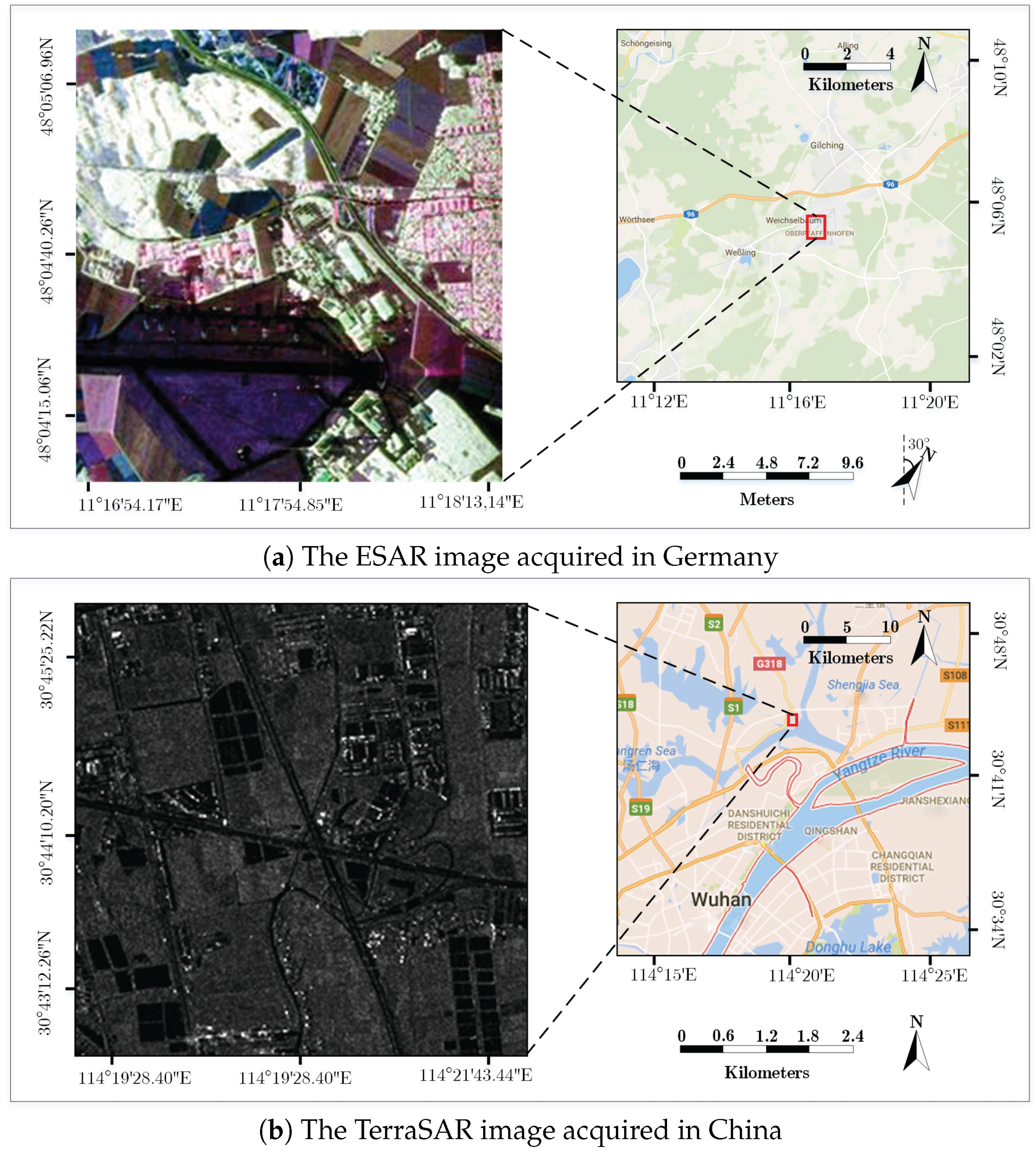
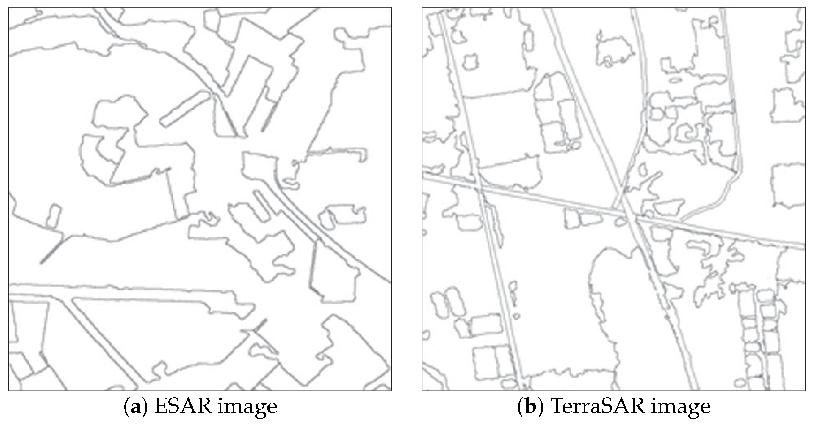
5.1. Experiment Data

To evaluate the performance of the proposed classification method, several experiments are conducted on ESAR and TerraSAR-X images. (1) As shown in Figure 7a, the ESAR image, acquired in Germany, has a dimension of $1300\times 1200$ pixels and a spatial resolution of 3 m × 2.2 m. (2) The second data, shown in Figure 7b, are acquired by TerraSAR from Wuhan, Hubei province, China; the dimension and spatial resolution are $1500\times 1500$ pixels and 1.25 m × 1.25 m, respectively. We use ArcGIS to label the experiment images into five categories, i.e., building, forest, farmland, road and others.

Figure 7. Experiment data.

5.2. Experiment Settings

As shown in Table 1, three types of features are extracted, i.e., intensity, polarization and texture features. For the intensity, the Haar and Grey histogram are included; the polarization feature consists of Pauli, SDHand Huynen; as for the texture, a filter bank consisting of 17 Gaussian filters is used to capture the texture feature. Notice that the TerraSAR image, used in our experiment, is of single polarization, and the extracted features only contain the intensity and texture.

Table 1. Three types of features are extracted for the experiment.

Attribute	Feature Type	Dimension
Intensity	Haar	7
	Grey	16
Polarization	Pauli	3
	SDH	9
	Huynen	3
Texture	Gaussian filters	17

Five experiments are designed for performance comparison, and the settings are described as follows.

Experiment 1: classification based on the CRF model alone: Firstly, 3 different thresholds are selected to construct a region pyramid. For the ESAR image, 0.2, 0.08 and 0.05 are set, and the corresponding region blocks are 1468, 3016 and 6134, respectively. For the TerraSAR image, the thresholds are set as 0.11, 0.08 and 0.06, and the segmentation blocks are 1898, 3629 and 7034, respectively. Secondly, half of those regions are used as training data and the others for testing. Thirdly, the spatial relationships of regions within each sub-layer of the region pyramid are model by the CRF. L-BFGS [33] is applied to estimate the parameters of the CRF model during the training process, and the min-sum algorithm is used for inference.

Experiment 2: classification based on CRF and boundary prior knowledge: The contour lines are detected by the method $gDet$-OWT-UCM, described in Section 3. To obtain the boundary prior knowledge, here those strong responses in UCM are retained, as shown in Figure 8. The boundary prior knowledge is calculated by Equation (8), and the corresponding linear weighted parameters are learned by training process.

Figure 8. Contour lines for boundary prior knowledge.

Experiment 3: classification combining CRF with the BN model: The CPT is shown in Table 2; Classes 1 to 5 correspond to the buildings, forests, farmland, roads and others. These conditional probabilities are set according to the results in Experiments 1 and 2. For ESAR data, for example, the probability 0.15, in Row 2 Column 3, represents the classification probability of farmland in the lower layer, conditioned on the forests in the upper layer.

Table 2. Conditional probability table.

Classes	ESAR Data					TerraSAR Data
	1	2	3	4	5	1	2	3	4	5
1	0.71	0.12	0.04	0.05	0.08	0.7	0.08	0.07	0.05	0.1
2	0.1	0.7	0.15	0.02	0.03	0.07	0.7	0.15	0.02	0.06
3	0.02	0.15	0.7	0.04	0.09	0.03	0.1	0.75	0.04	0.08
4	0.05	0.02	0.03	0.82	0.08	0.1	0.04	0.03	0.8	0.03
5	0.08	0.06	0.06	0.1	0.7	0.1	0.08	0.04	0.1	0.68

Experiment 4: classification by SVM: For comparison purposes, Support Vector Machine (SVM) [34] is used to classify the oversegmentation regions; the settings for the feature extraction are the same as Experiment 1. Half of the obtained regions are randomly selected for testing data and the others for testing.

Experiment 5: CRF model with mean shift and Potts prior: To verify the segmentation efficiency of $gDet$-OWT-UCM, the CRF model is built based on the mean shift segmentation and Potts’ prior [35]. The minimum block size is $200\times 200$, and the obtained regions are 3370 and 3955 for ESAR and TerraSAR data, respectively. Other settings for CRF are the same as Experiment 1.

5.3. Results and Analysis

Figure 9 and Figure 10 qualitatively illustrate the classification results of each experiment on ESAR and TerraSAR images. To further quantitatively compare the performance, Table 3 and Table 4 list the confusion matrices of the classification results.

(1)

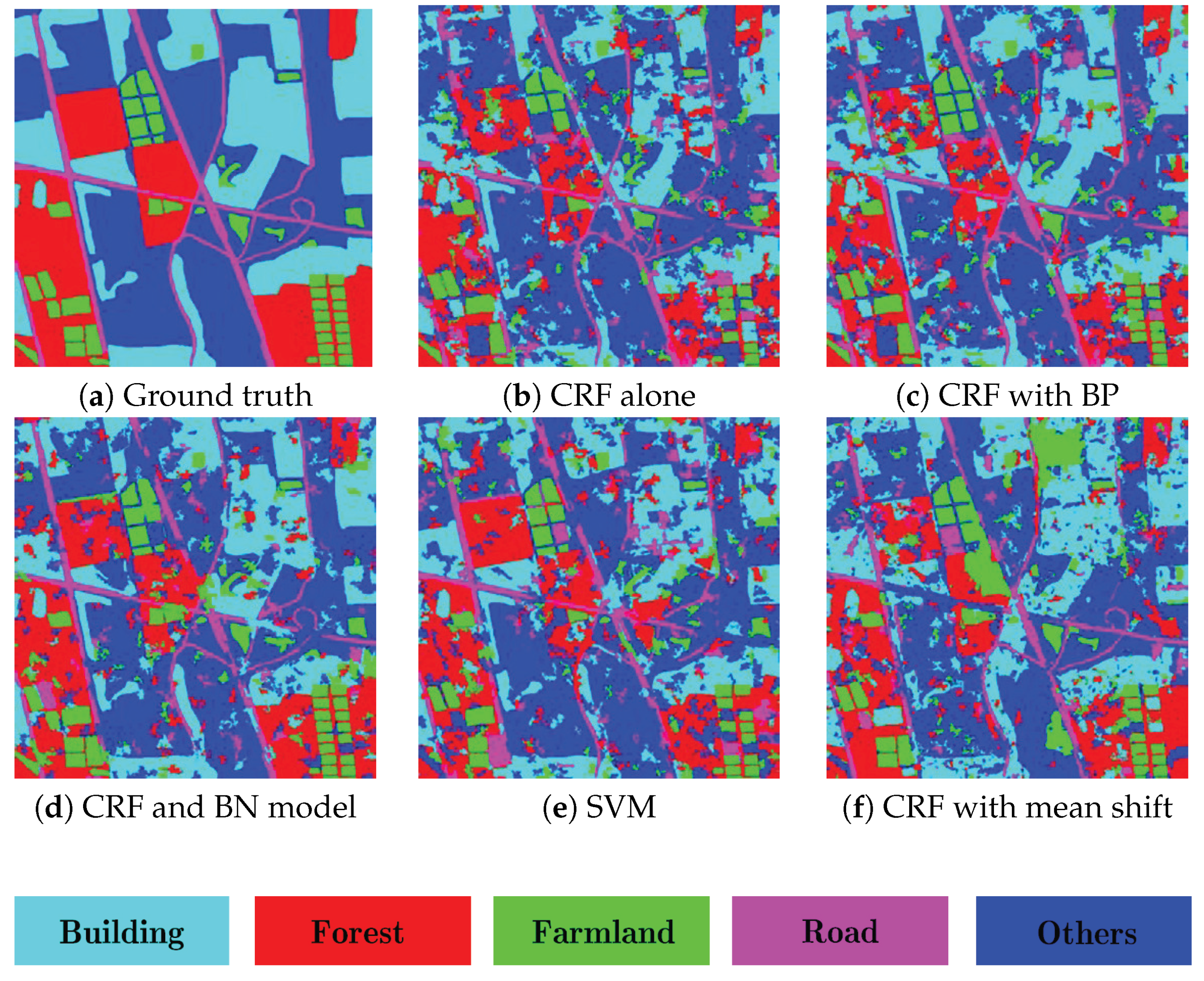
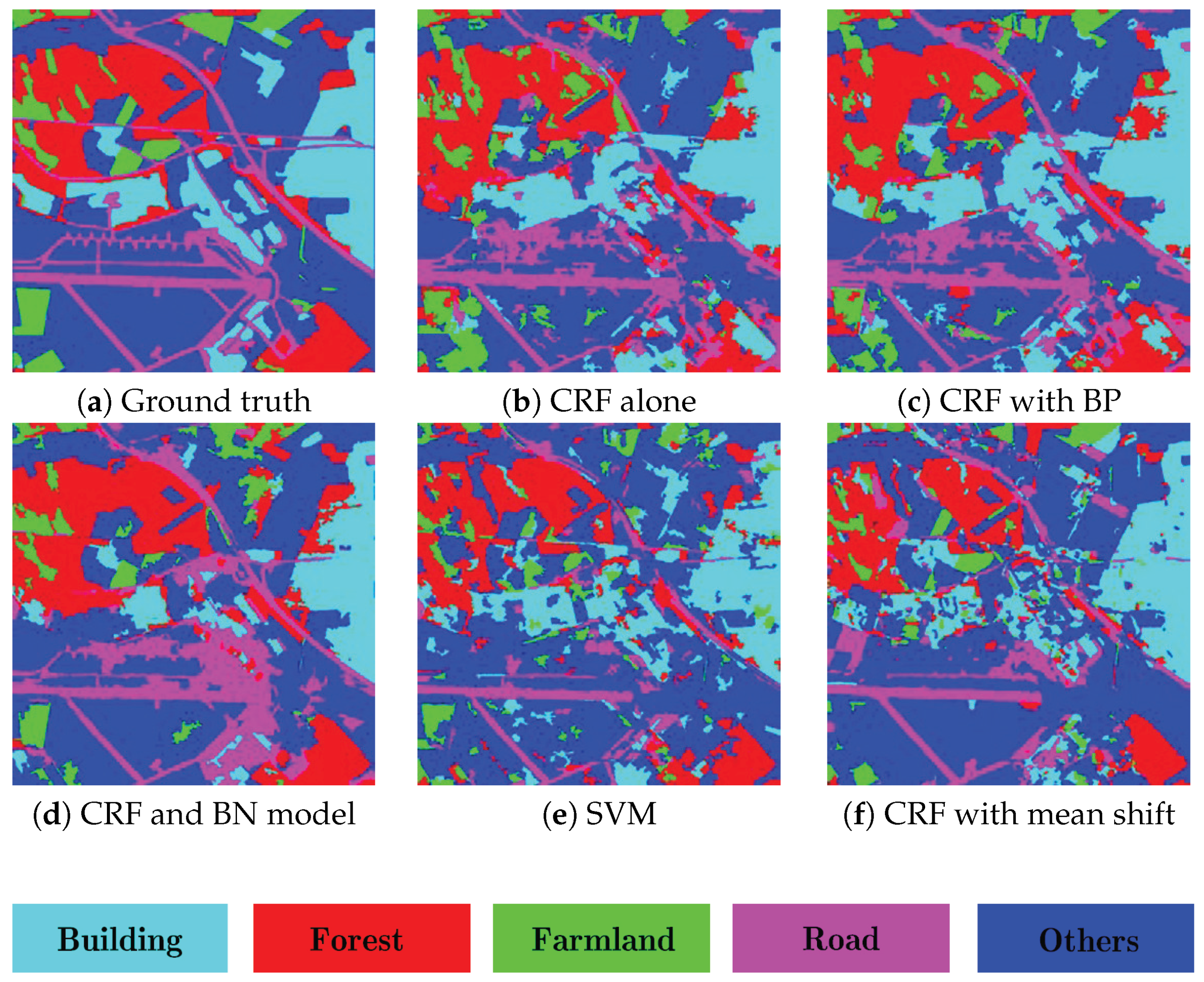
For the ESAR data, the average classification accuracy of CRF model alone [36] is about 70.7%, as shown in Figure 9b. When the boundary prior knowledge is incorporated into CRF model, the average accuracy is up to 72.8%, the classification performance is improved about 2%, especially those areas around the boundary, as shown in Figure 9c. The performance of the proposed method is more promising, as shown in Figure 9d. Compared with the CRF model alone and CRF with boundary prior approaches, the accuracy is improved about 6% and 3.8%, respectively. This is because of the additional contextual knowledge, namely the causal dependencies between adjacent layers are integrated into the proposed classification framework. Figure 9e,f presents the results of SVM [34] and the CRF model based on mean shift [35]; the comparable performance demonstrates the effectiveness of the segmentation algorithm used in this paper.

(2)

Figure 10 displays the results on the TerraSAR image. The average classification accuracy of the proposed method is about 81.2%, which is better than the CRF model alone, 73.0%, and CRF with boundary prior, 76.1%. These experimental results also demonstrate that the incorporation of additional prior knowledge, namely the causal connections modeled by BN, is a benefit to the enhancement of classification performance. Moreover, note that the accuracy of CRF with boundary prior knowledge is improved about 3% compared with the CRF model alone, and the recognition ability on those sub-regions, e.g., forest, buildings, is improved effectively, which verifies the effectiveness of the incorporation of the boundary prior knowledge.

(3)

Since the causal relationships between adjacent layers, as well as the boundary prior knowledge are integrated into the proposed method, the computational cost of our method is relatively higher than those methods used for comparison purposes.

Figure 9. Classification results of ESAR image. (a) The ground truth; (b–d) the results by the CRF model alone, CRF with boundary prior knowledge, CRF and the BN model, respectively; (e,f) the results by SVM and CRF with mean shift.

Figure 10. Classification results of TerraSAR image. (a) The ground truth; (b–d) the results by the CRF model alone, CRF with boundary prior knowledge, CRF and the BN model, respectively; (e,f) the results by SVM and CRF with mean shift.

Table 3. Confusion matrix for the classification results of ESAR data.

Method	Category	Building	Forest	Farmland	Road	Others	Average
	Building	0.7305	0.1505	0.0034	0.0296	0.086
	Forest	0.1374	0.7203	0.0732	0.041	0.0282
Experiment 1	Farmland	0.0118	0.1966	0.581	0.0146	0.196	0.7066
	Road	0.0887	0.0706	0.0034	0.6302	0.2071
	Others	0.0487	0.0341	0.0649	0.1193	0.733
	Building	0.8164	0.1083	0.0047	0.0214	0.0493
	Forest	0.1007	0.802	0.0419	0.0182	0.0372
Experiment 3	Farmland	0.0136	0.2423	0.5156	0.014	0.2145	0.7284
	Road	0.0964	0.0578	0.0084	0.6258	0.2116
	Others	0.0623	0.0428	0.0544	0.1125	0.728
	Building	0.6613	0.1522	0.0076	0.1025	0.0763
	Forest	0.0274	0.8329	0.0468	0.033	0.0598
Experiment 5	Farmland	0.0028	0.1201	0.6069	0.0092	0.261	0.7669
	Road	0.0197	0.0495	0.0031	0.7602	0.1675
	Others	0.0165	0.0266	0.0299	0.1251	0.802
	Building	0.7728	0.0666	0.0255	0.0166	0.1185
	Forest	0.0693	0.7109	0.0179	0.0043	0.1975
Experiment 4	Farmland	0.0461	0.1376	0.4655	0.0057	0.3451	0.7127
	Road	0.063	0.049	0.0286	0.4049	0.4545
	Others	0.0664	0.0379	0.037	0.0429	0.8158
	Building	0.7884	0.0356	0.0294	0.0321	0.1246
	Forest	0.0841	0.6325	0.0296	0.0455	0.2083
Experiment 2	Farmland	0.0329	0.1685	0.4345	0.0362	0.3297	0.7218
	Road	0.0698	0.0463	0.0255	0.5104	0.3479
	Others	0.0458	0.0201	0.0268	0.0624	0.8449

Table 4. Confusion matrix for the classification results of TerraSAR data.

Method	Category	Building	Forest	Farmland	Road	Others	Average
	Building	0.673	0.0513	0.0369	0.0436	0.1952
	Forest	0.0927	0.6679	0.0321	0.0355	0.1718
Experiment 1	Farmland	0.0725	0.011	0.6573	0.0494	0.2099	0.7295
	Road	0.1005	0.053	0.0419	0.6891	0.1155
	Others	0.0497	0.0471	0.0394	0.0359	0.8278
	Building	0.7706	0.0363	0.0419	0.0316	0.1196
	Forest	0.088	0.665	0.043	0.0377	0.1663
Experiment 3	Farmland	0.0623	0.0372	0.7486	0.0284	0.1235	0.7607
	Road	0.0945	0.0373	0.0317	0.7699	0.0666
	Others	0.0595	0.0481	0.0423	0.0422	0.8079
	Building	0.8005	0.0454	0.0371	0.0145	0.1025
	Forest	0.0315	0.7984	0.0413	0.0241	0.1047
Experiment 5	Farmland	0.0328	0.0309	0.8383	0.0433	0.0546	0.8117
	Road	0.0554	0.02	0.0347	0.7905	0.0993
	Others	0.0517	0.0434	0.0309	0.0284	0.8455
	Building	0.7069	0.0649	0.0403	0.039	0.1489
	Forest	0.0546	0.714	0.04	0.0326	0.1587
Experiment 4	Farmland	0.0151	0.0621	0.7112	0.0965	0.1151	0.7422
	Road	0.0729	0.0663	0.0529	0.6292	0.1787
	Others	0.0573	0.0553	0.0323	0.0421	0.813
	Building	0.764	0.0381	0.0391	0.0316	0.1272
	Forest	0.0697	0.7035	0.0794	0.0236	0.1238
Experiment 2	Farmland	0.0911	0.0567	0.7054	0.0746	0.0722	0.7403
	Road	0.0617	0.0323	0.0365	0.6317	0.2379
	Others	0.0766	0.0392	0.0912	0.0204	0.7726

6. Discussion

To achieve a finer classification result, we incorporate more prior knowledge into our classification framework by constructing a multilayer region pyramid, where CRF and BN are used to model the spatial relationships and adjacent causal connections. To further improve the accuracy and to apply the proposed method in practical applications, the following aspects should be taken into account.

(1)

The number of layers for constructing a region pyramid plays an important role in performance enhancement, and how to select the optimal number of layers is an issue that should be further studied. In theory, the more layers we select, the higher the accuracy that will be achieved. However, an optimum selection is intractable because we should ensure the existence of the classification probabilities of those sub-regions conditioned on their parents’ regions in the upper layer. Therefore, this issue should be further studied for the enhancement of the performance.

(2)

There are several hyperparameters in the process of oversegmentation, e.g., the scale for the extraction of local edges, etc. These hyperparameters, which like the concept of receptive field in the deep learning community, have some impact on the classification performance. However, how to select an optimum setting still needs to be addressed.

(3)

Since there are several parameters that should be learned in our proposed method, a higher computational cost should be paid. Consequently, we should make a tradeoff between the computational cost and classification accuracy, especially for the selection of the number of layers in forming a region pyramid.

(4)

Combining more prior knowledge with the image data itself is a benefit to the accuracy improvement. Therefore, more prior knowledge is encouraged to be incorporated into this classification framework to further performance enhancement.

(5)

The overfitting problem should also be considered in the case of insufficient training samples. In this paper, a uniform distribution is used to model the prior probability. To further improve the generalization, other strategies, like the solution in [37], should be taken into account.

7. Conclusions

This paper has presented a hierarchical classification method for SAR images. In contrast to existing multiscale approaches, which concentrate on the development of contextual information within a sub-layer, the proposed classifying framework explores the causal connections between adjacent layers as prior knowledge to facilitate robust and effective classification. To integrate the causalities, a multilayer region pyramid is first constructed by multiscale oversegmentation, and then, both the Bayesian Network (BN) and Conditional Random Field (CRF) are used to model prior knowledge, where CRF models the spatial relationships among regions within sub-layers and BN captures the causal connections between adjacent layers. Experiments conducted on real SAR images demonstrate the superiority of the proposed method, and the accuracy is improved by about 3%.

References

- Moreira, A.; Prats-Iraola, P.; Younis, M.; Krieger, G.; Hajnsek, I.; Papathanassiou, K.P. A tutorial on synthetic aperture radar. IEEE Geosci. Remote Sens. Mag. 2013, 1, 6–43. [Google Scholar] [CrossRef]
- Huynen, J.R. Phenomenological theory of radar targets. In Electromagnetic Scattering; Academic Press: New York, NY, USA, 1970; pp. 653–712. [Google Scholar]
- Cloude, S. Group theory and polarisation algebra. Optik 1986, 75, 26–36. [Google Scholar]
- Krogager, E. New decomposition of the radar target scattering matrix. Electron. Lett. 1990, 26, 1525–1527. [Google Scholar] [CrossRef]
- Freeman, A.; Durden, S.L. A three-component scattering model for polarimetric SAR data. IEEE Trans. Geosci. Remote Sens. 1998, 36, 963–973. [Google Scholar] [CrossRef]
- Yamaguchi, Y.; Moriyama, T.; Ishido, M.; Yamada, H. Four-component scattering model for polarimetric SAR image decomposition. IEEE Trans. Geosci. Remote Sens. 2005, 43, 1699–1706. [Google Scholar] [CrossRef]
- Touzi, R. Target Scattering Decomposition in Terms of Roll-Invariant Target Parameters. IEEE Trans. Geosci. Remote Sens. 2007, 45, 73–84. [Google Scholar] [CrossRef]
- An, W.; Cui, Y.; Yang, J. Three-Component Model-Based Decomposition for Polarimetric SAR Data. IEEE Trans. Geosci. Remote Sens. 2010, 48, 2732–2739. [Google Scholar]
- Sato, A.; Yamaguchi, Y.; Singh, G.; Park, S.E. Four-Component Scattering Power Decomposition with Extended Volume Scattering Model. IEEE Geosci. Remote Sens. Lett. 2012, 9, 166–170. [Google Scholar] [CrossRef]
- He, C.; Li, S.; Liao, Z.X.; Liao, M.S. Texture classification of PolSAR data based on sparse coding of wavelet polarization textons. IEEE Geosci. Remote Sens. 2013, 8, 4576–4590. [Google Scholar] [CrossRef]
- Kandaswamy, U.; Adjeroh, D.A.; Lee, M.C. Efficient Texture Analysis of SAR Imagery. IEEE Trans. Geosci. Remote Sens. 2005, 43, 2075–2083. [Google Scholar] [CrossRef]
- Akbarizadeh, G. A New Statistical-Based Kurtosis Wavelet Energy Feature for Texture Recognition of SAR Images. IEEE Trans. Geosci. Remote Sens. 2012, 50, 4358–4368. [Google Scholar] [CrossRef]
- Planinsic, P.; Singh, J.; Gleich, D. SAR Image Categorization Using Parametric and Nonparametric Approaches Within a Dual Tree CWT. IEEE Geosci. Remote Sens. Lett. 2014, 11, 1757–1761. [Google Scholar] [CrossRef]
- Dekker, R.J. Texture analysis and classification of ERS SAR images for map updating of urban areas in The Netherlands. IEEE Trans. Geosci. Remote Sens. 2003, 41, 1950–1958. [Google Scholar] [CrossRef]
- Dai, D.; Yang, W.; Sun, H. Multilevel Local Pattern Histogram for SAR Image Classification. IEEE Geosci. Remote Sens. Lett. 2011, 8, 225–229. [Google Scholar] [CrossRef]
- Deng, Q.; Chen, Y.; Zhang, W.; Yang, J. Colorization for Polarimetric SAR Image Based on Scattering Mechanisms. In Proceedings of the 2008 Congress on Image and Signal Processing, Sanya, China, 27–30 May 2008; pp. 697–701.
- Turner, D.; Woodhouse, I.H. An Icon-Based Synoptic Visualization of Fully Polarimetric Radar Data. Remote Sens. 2012, 4, 648–660. [Google Scholar] [CrossRef]
- Uhlmann, S.; Kiranyaz, S. Integrating Color Features in Polarimetric SAR Image Classification. IEEE Trans. Geosci. Remote Sens. 2014, 52, 2197–2216. [Google Scholar] [CrossRef]
- Golparvar-Fard, M.; Balali, V.; de la Garza, J.M. Segmentation and recognition of highway assets using image-based 3D point clouds and semantic Texton forests. J. Comput. Civ. Eng. 2012, 29, 04014023. [Google Scholar] [CrossRef]
- Balali, V.; Golparvar-Fard, M. Segmentation and recognition of roadway assets from car-mounted camera video streams using a scalable non-parametric image parsing method. Autom. Constr. 2015, 49, 27–39. [Google Scholar] [CrossRef]
- Li, S.Z. Markov Random Field Modeling in Image Analysis; Springer Science & Business Media: Berlin, Germany, 2009. [Google Scholar]
- Lafferty, J.D.; Mccallum, A.; Pereira, F.C.N. Conditional Random Fields: Probabilistic Models for Segmenting and Labeling Sequence Data. In Proceedings of the Eighteenth International Conference on Machine Learning (ICML), Williamstown, MA, USA, 28 June–1 July 2001; pp. 282–289.
- Nielsen, T.D.; Jensen, F.V. Bayesian Networks and Decision Graphs; Springer Science & Business Media: Berlin, Germany, 2009. [Google Scholar]
- D’Elia, C.; Ruscino, S.; Abbate, M.; Aiazzi, B.; Baronti, S.; Alparone, L. SAR Image Classification Through Information-Theoretic Textural Features, MRF Segmentation, and Object-Oriented Learning Vector Quantization. IEEE J. Sel. Top. Appl. Earth Obs. Remote Sens. 2014, 7, 1116–1126. [Google Scholar] [CrossRef]
- Voisin, A.; Krylov, V.A.; Moser, G.; Serpico, S.B.; Zerubia, J. Classification of Very High Resolution SAR Images of Urban Areas Using Copulas and Texture in a Hierarchical Markov Random Field Model. IEEE Geosci. Remote Sens. Lett. 2013, 10, 96–100. [Google Scholar] [CrossRef]
- Su, X.; He, C.; Feng, Q.; Deng, X.; Sun, H. A Supervised Classification Method Based on Conditional Random Fields With Multiscale Region Connection Calculus Model for SAR Image. IEEE Geosci. Remote Sens. Lett. 2011, 8, 497–501. [Google Scholar] [CrossRef]
- Zhang, G.; Jia, X. Simplified Conditional Random Fields with Class Boundary Constraint for Spectral-Spatial Based Remote Sensing Image Classification. IEEE Geosci. Remote Sens. Lett. 2012, 9, 856–860. [Google Scholar] [CrossRef]
- Ding, Y.; Li, Y.; Yu, W. SAR Image Classification Based on CRFs with Integration of Local Label Context and Pairwise Label Compatibility. IEEE J. Sel. Top. Appl. Earth Obs. Remote Sens. 2014, 7, 300–306. [Google Scholar] [CrossRef]
- Mortensen, E.N.; Jia, J. Real-Time Semi-Automatic Segmentation Using a Bayesian Network. In Proceedings of the IEEE Conference on Computer Vision and Pattern Recognition, New York, NY, USA, 17–22 June 2006; pp. 1007–1014.
- Arbelaez, P.; Maire, M.; Fowlkes, C.; Malik, J. Contour Detection and Hierarchical Image Segmentation. IEEE Trans. Pattern Anal. Mach. Intell. 2011, 33, 898–916. [Google Scholar] [CrossRef] [PubMed]
- Arbelaez, P. Boundary Extraction in Natural Images Using Ultrametric Contour Maps. In Proceedings of the Conference on Computer Vision and Pattern Recognition Workshop, New York, NY, USA, 17–22 June 2006; p. 182.
- Hutter, F.; Hoos, H.H.; Stutzle, T. Efficient stochastic local search for MPE solving. In Proceedings of the Nineteenth International Joint Conference on Artificial Intelligence, Edinburgh, UK, 30 July–5 August 2005; pp. 169–174.
- Liu, D.C.; Nocedal, J. On the limited memory BFGS method for large scale optimization. Math. Program. 1989, 45, 503–528. [Google Scholar] [CrossRef]
- Maghsoudi, Y.; Collins, M.J.; Leckie, D.G. Radarsat-2 Polarimetric SAR Data for Boreal Forest Classification Using SVM and a Wrapper Feature Selector. IEEE J. Sel. Top. Appl. Earth Obs. Remote Sens. 2013, 6, 1531–1538. [Google Scholar] [CrossRef]
- Comaniciu, D.; Meer, P. Mean shift: A robust approach toward feature space analysis. IEEE Trans. Pattern Anal. Mach. Intell. 2002, 24, 603–619. [Google Scholar] [CrossRef]
- Zhang, P.; Li, M.; Wu, Y.; Li, H. Hierarchical Conditional Random Fields Model for Semisupervised SAR Image Segmentation. IEEE Trans. Geosci. Remote Sens. 2015, 53, 4933–4951. [Google Scholar] [CrossRef]
- Salazar, A.; Safont, G.; Vergara, L. Surrogate techniques for testing fraud detection algorithms in credit card operations. In Proceedings of the 2014 IEEE International Carnahan Conference on Security Technology (ICCST), Rome, Italy, 13–16 October 2014; pp. 1–6.
© 2017 by the authors; licensee MDPI, Basel, Switzerland. This article is an open access article distributed under the terms and conditions of the Creative Commons Attribution (CC BY) license (http://creativecommons.org/licenses/by/4.0/).