
Assessment of Regional Vegetation Response to Climate Anomalies: A Case Study for Australia Using GIMMS NDVI Time Series between 1982 and 2006

 , ,
, ,
Abstract
:
1. Introduction
2. Materials and Methods
2.1. Study Area and Data
2.1.1. Study Area
2.1.2. Land Cover Data, NDVI and Climate Time Series
NDVI Data
Climate Data
Land Cover Data
2.2. Methodology
- The vegetation response and climate anomaly were extracted from the NDVI and climate time series (Section 2.2.1).
- Stability metrics were calculated over a running window of the anomaly time series, resulting in new time series of stability metrics.
- In order to quantify how much the stability changes over time and whether the stability generally increases or decreases, two non-stationarity metrics were defined: the magnitude and direction of stability change (Section 2.2.2).
- The non-stationarity of each stability metric was linked to vegetation and environmental characteristics to enhance their interpretation.
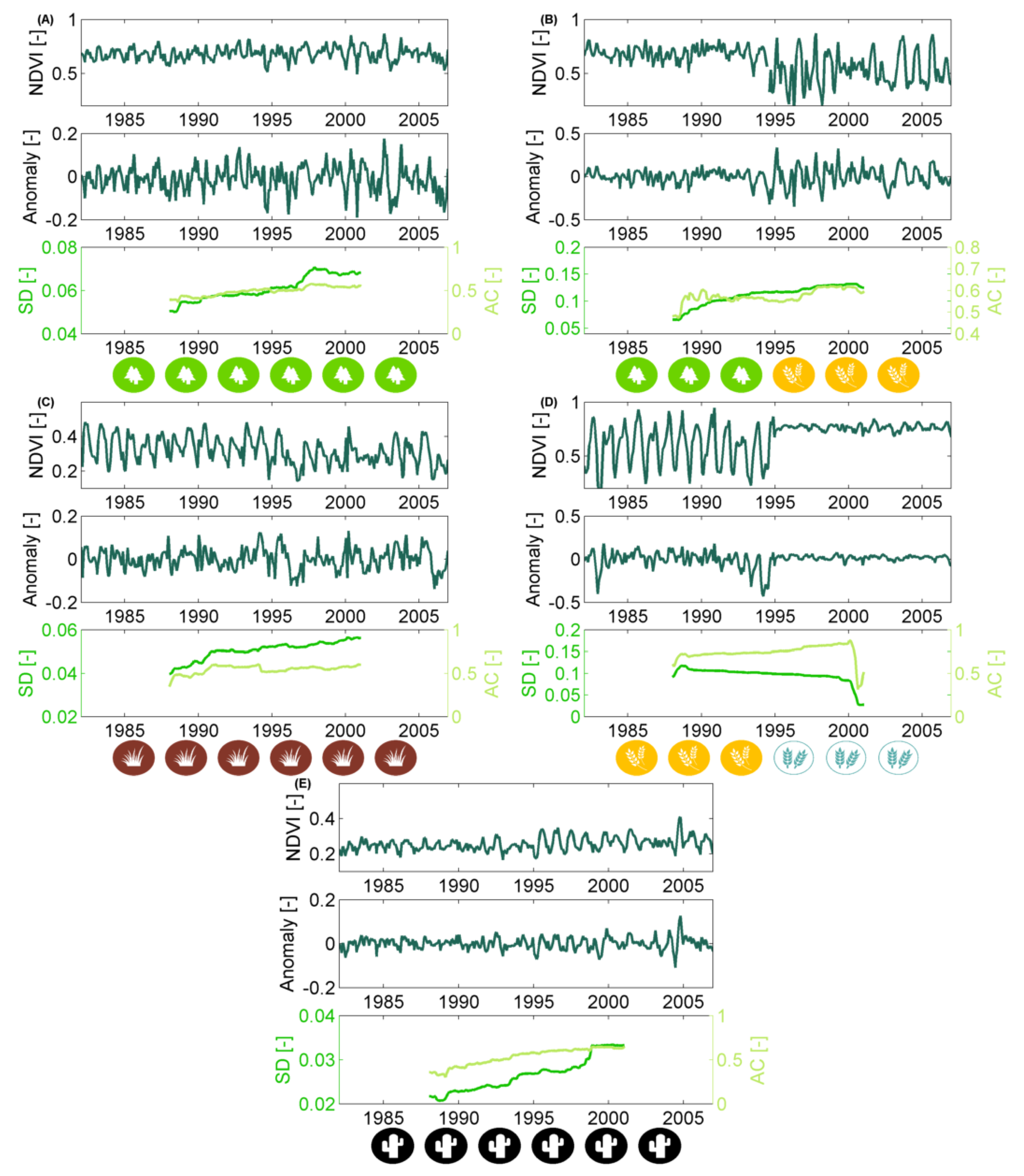
2.2.1. Non-Stationary Anomaly Time Series
2.2.2. Quantifying Non-Stationarity of the Short-Term Vegetation Response
3. Results
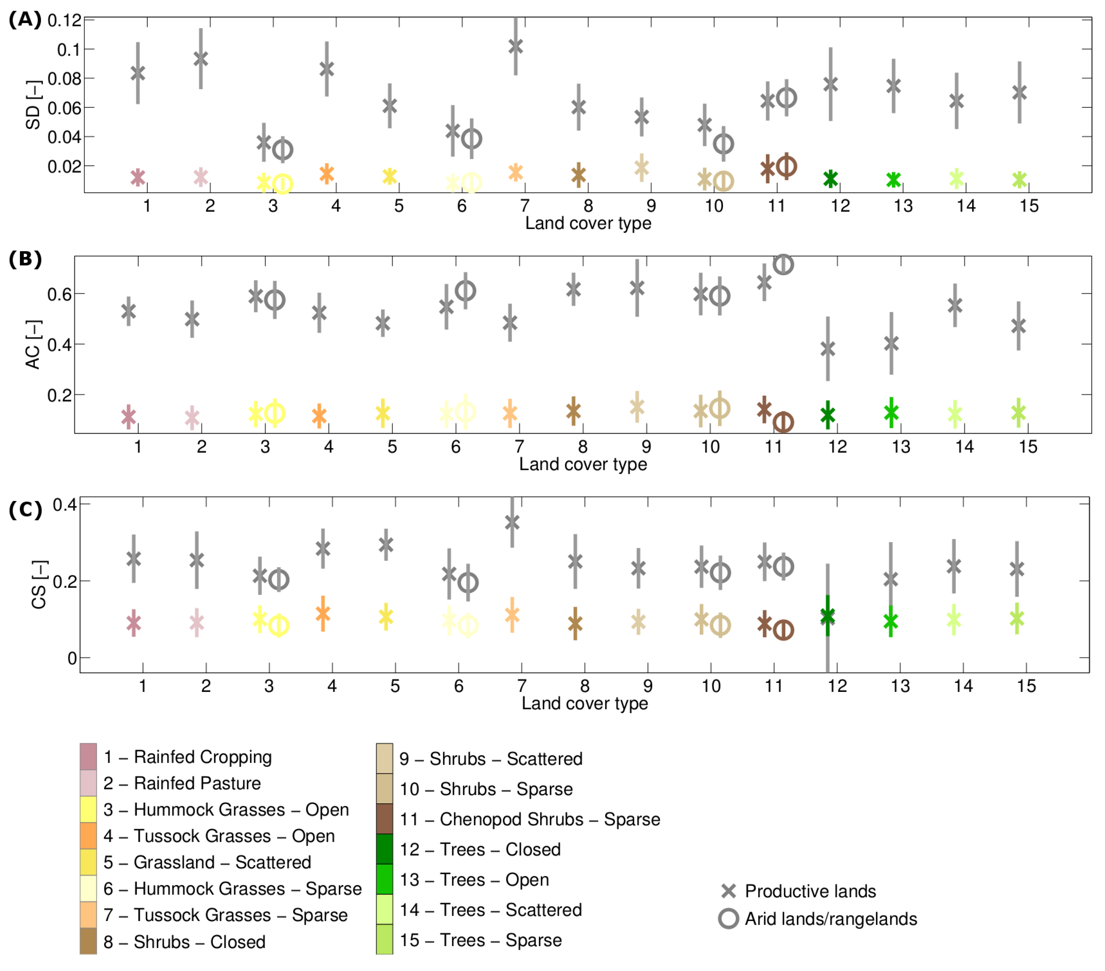
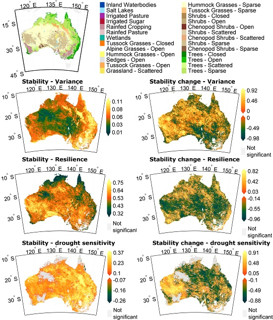
3.1. Stability Derived over the Complete Time Period
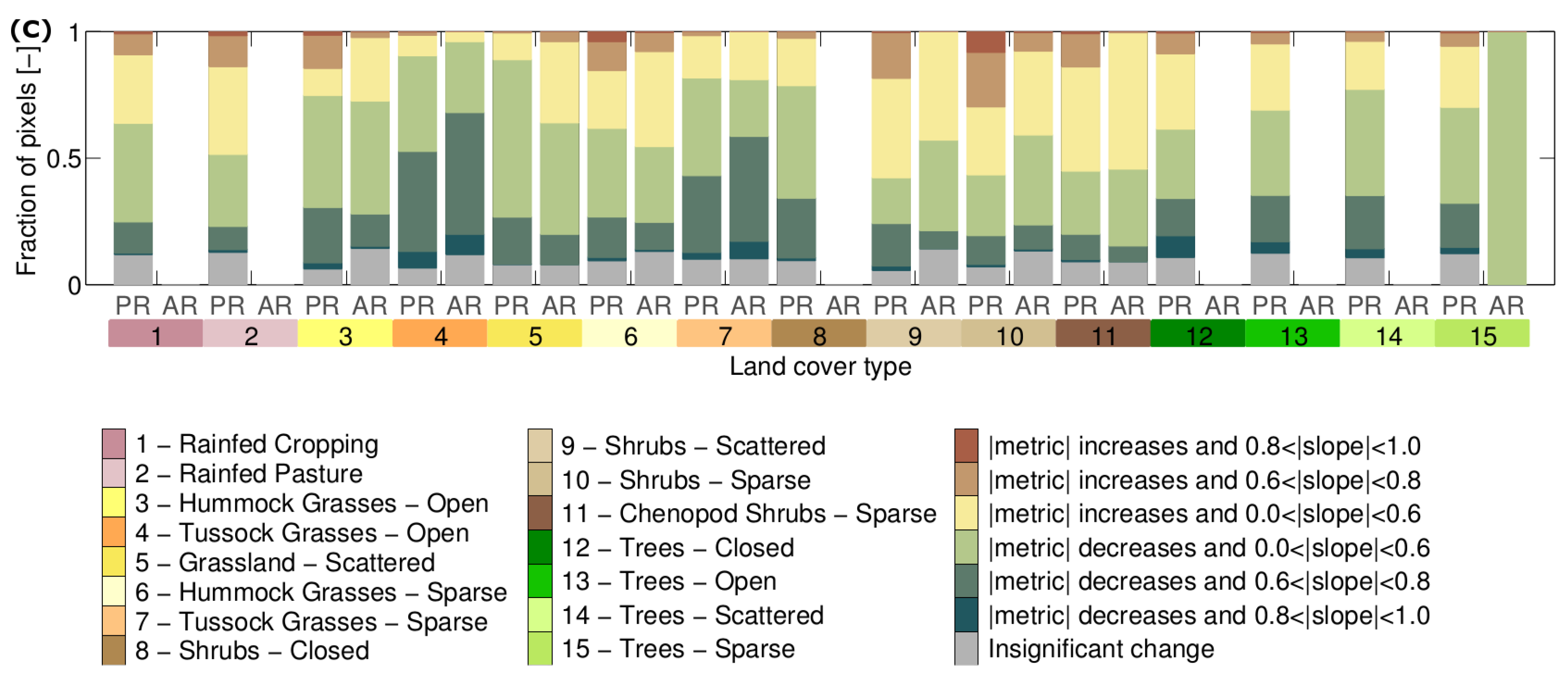
3.2. How Much Does Vegetation Stability Change over Time?
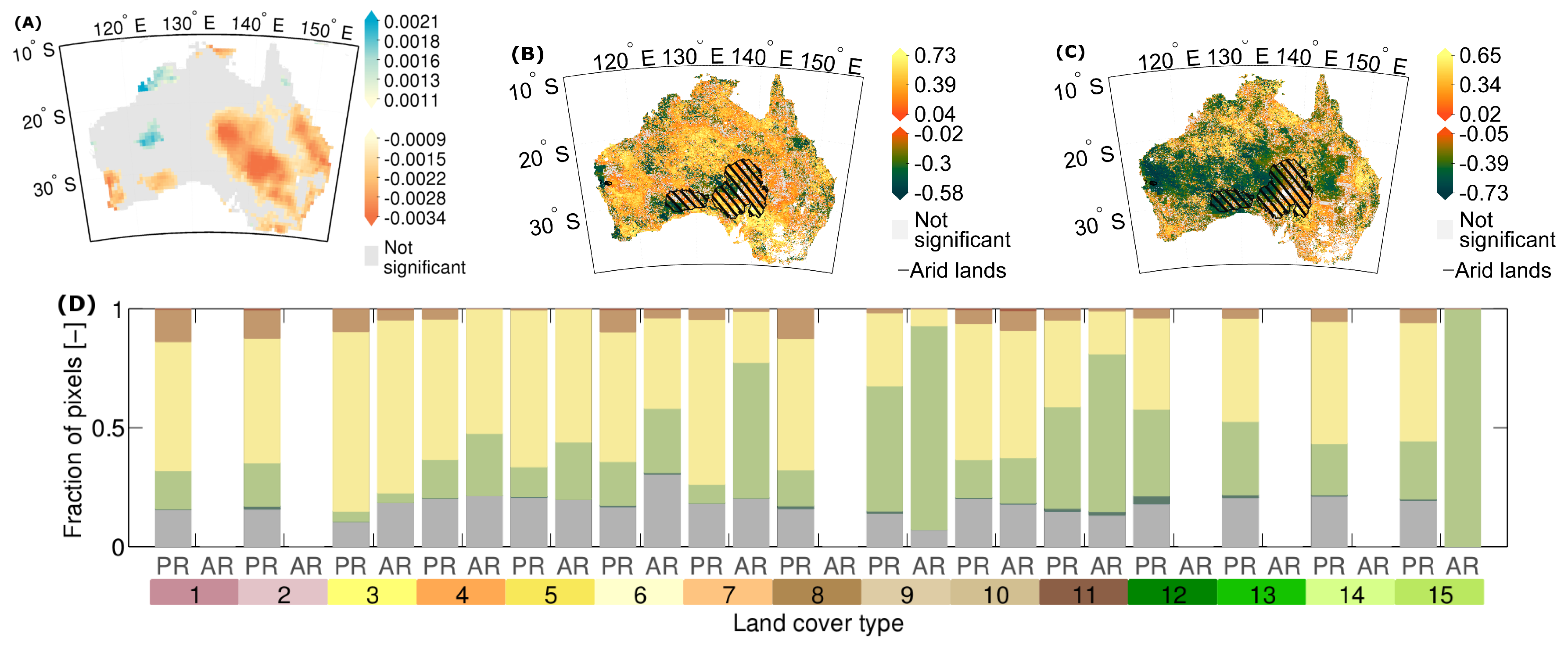
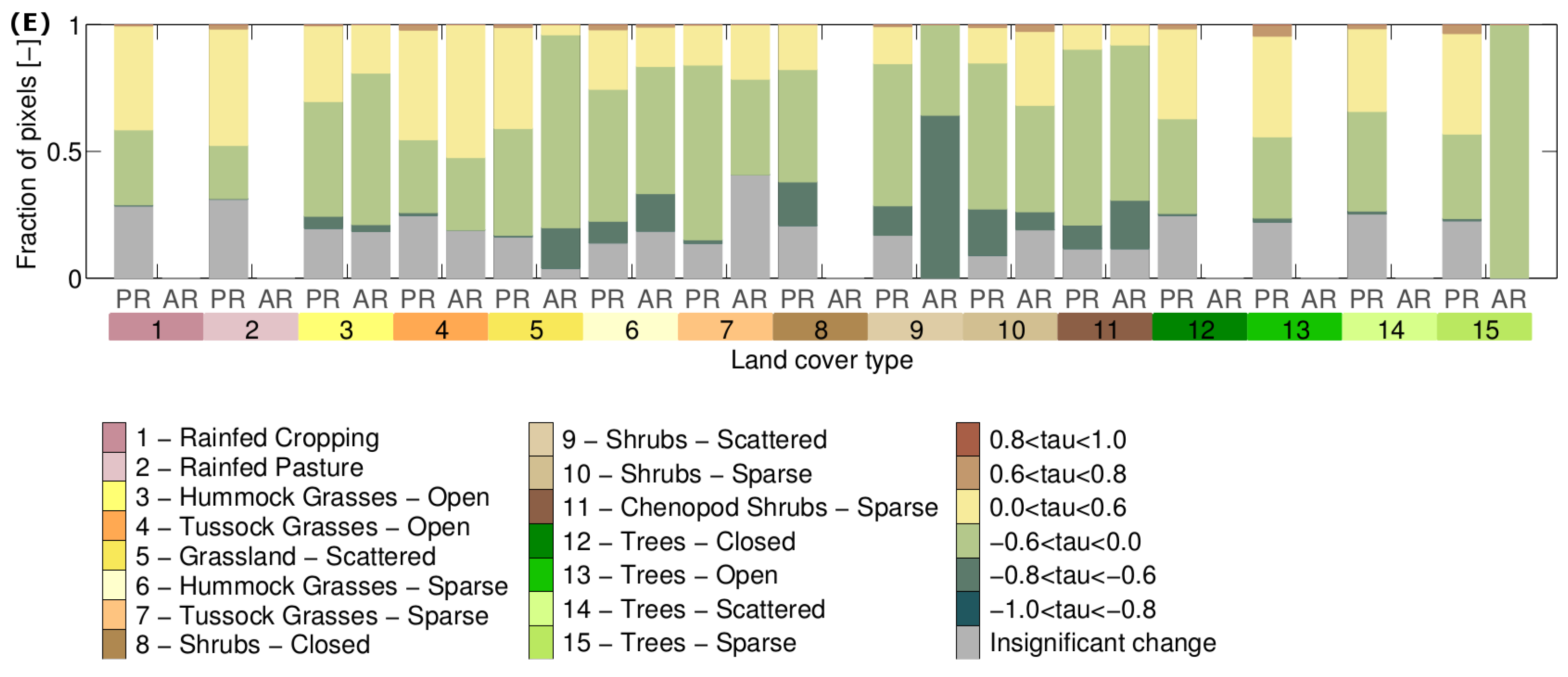
3.3. Is Vegetation Response Becoming More/Less Stable over Time?
4. Discussion
5. Conclusions
Acknowledgments
Author Contributions
Conflicts of Interest
References
- Malinga, R.; Gordon, L.J.; Jewitt, G.; Lindborg, R. Mapping ecosystem services across scales and continents: A review. Ecosyst. Serv. 2015, 13, 57–63. [Google Scholar] [CrossRef]
- Intergovernmental Panel on Climate Change (IPCC). Managing the Risks of Extreme Events and Disasters to Advance Climate Change Adaptation; A Special Report of Working Groups I and II of the Intergovernmental Panel on Climate Change; Chapter Summary for Policymakers; Cambridge University Press: Cambridge, UK; New York, NY, USA, 2012; pp. 1–19. [Google Scholar]
- Pimm, S. The complexity and stability of ecosystems. Nature 1984, 307, 321–326. [Google Scholar] [CrossRef]
- Pettorelli, N.; Vik, J.; Mysterud, A.; Gaillard, J.; Tucker, C.; Stenseth, N. Using the satellite-derived NDVI to assess ecological responses to environmental change. Trends Ecol. Evol. 2005, 20, 503–510. [Google Scholar] [CrossRef] [PubMed]
- De Keersmaecker, W.; Lhermitte, S.; Honnay, O.; Farifteh, J.; Somers, B.; Coppin, P. How to measure ecosystem stability? An evaluation of the reliability of stability metrics based on remote sensing time series across the major global ecosystems. Glob. Chang. Biol. 2014, 20, 2149–2161. [Google Scholar] [CrossRef] [PubMed]
- De Keersmaecker, W.; Lhermitte, S.; Tits, L.; Honnay, O.; Somers, B.; Coppin, P. Resilience and the reliability of spectral entropy to assess ecosystem stability. Glob. Chang. Biol. 2015. [Google Scholar] [CrossRef] [PubMed]
- Milly, P.C.D.; Betancourt, J.; Falkenmark, M.; Hirsch, R.M.; Kundzewicz, Z.W.; Lettenmaier, D.P.; Stouffer, R.J. Stationarity is dead: Whither water management? Science 2008, 319, 573–574. [Google Scholar] [CrossRef] [PubMed]
- Lenton, T.M. Early warning of climate tipping points. Nat. Clim. Chang. 2011, 1, 201–209. [Google Scholar] [CrossRef]
- Dakos, V.; Carpenter, S.; Brock, W.; Ellison, A.; Guttal, V.; Ives, A.; Kéfi, S.; Livina, V.; Seekell, D.; van Nes, E.; et al. Methods for detecting early warnings of critical transitions in time series illustrated using simulated ecological data. PLoS ONE 2012, 7, e41010. [Google Scholar] [CrossRef] [PubMed]
- Verbesselt, J.; Umlauf, N.; Hirota, M.; Holmgren, M.; Van Nes, E.H.; Herold, M.; Zeileis, A.; Scheffer, M. Remotely sensed resilience of tropical forests. Nat. Clim. Chang. 2016. [Google Scholar] [CrossRef]
- Scheffer, M.; Carpenter, S.; Foley, J.A.; Folke, C.; Walker, B. Catastrophic shifts in ecosystems. Nature 2001, 413, 591–596. [Google Scholar] [CrossRef] [PubMed]
- De Jong, R.; Verbesselt, J.; Schaepman, M.E.; de Bruin, S. Trend changes in global greening and browning: Contribution of short-term trends to longer-term change. Glob. Chang. Biol. 2012, 18, 642–655. [Google Scholar] [CrossRef]
- Donohue, R.J.; Mcvicar, T.; Roderick, M.L. Climate-related trends in Australian vegetation cover as inferred from satellite observations, 1981–2006. Glob. Chang. Biol. 2009, 15, 1025–1039. [Google Scholar] [CrossRef]
- Dardel, C.; Kergoat, L.; Hiernaux, P.; Mougin, E.; Grippa, M.; Tucker, C. Re-greening Sahel: 30 years of remote sensing data and field observations (Mali, Niger). Remote Sens. Environ. 2014, 140, 350–364. [Google Scholar] [CrossRef]
- Herrmann, S.M.; Anyamba, A.; Tucker, C.J. Recent trends in vegetation dynamics in the African Sahel and their relationship to climate. Glob. Environ. Chang. 2005, 15, 394–404. [Google Scholar] [CrossRef]
- Fensholt, R.; Langanke, T.; Rasmussen, K.; Reenberg, A.; Prince, S.D.; Tucker, C.; Scholes, R.J.; Le, Q.B.; Bondeau, A.; Eastman, R.; et al. Greenness in semi-arid areas across the globe 1981–2007—An Earth Observing Satellite based analysis of trends and drivers. Remote Sens. Environ. 2012, 121, 144–158. [Google Scholar] [CrossRef]
- Heumann, B.W.; Seaquist, J.; Eklundh, L.; Jönsson, P. AVHRR derived phenological change in the Sahel and Soudan, Africa, 1982–2005. Remote Sens. Environ. 2007, 108, 385–392. [Google Scholar] [CrossRef]
- Fensholt, R.; Rasmussen, K. Analysis of trends in the Sahelian rain-use efficiency using GIMMS NDVI, RFE and GPCP rainfall data. Remote Sens. Environ. 2011, 115, 438–451. [Google Scholar] [CrossRef]
- Piao, S.; Nan, H.; Huntingford, C.; Ciais, P.; Friedlingstein, P.; Sitch, S.; Peng, S.; Ahlström, A.; Canadell, J.G.; Cong, N.; et al. Evidence for a weakening relationship between interannual temperature variability and northern vegetation activity. Nat. Commun. 2014, 5. [Google Scholar] [CrossRef] [PubMed]
- De Keersmaecker, W.; Lhermitte, S.; Tits, L.; Honnay, O.; Somers, B.; Coppin, P. A model quantifying global vegetation resistance and resilience against short-term climate anomalies and their relation with vegetation cover. Glob. Ecol. Biogeogr. 2015, 24, 539–548. [Google Scholar] [CrossRef]
- McAlpine, C.; Syktus, J.; Ryan, J.; Deo, R.; McKeon, G.; McGowan, H.; Phinn, S. A continent under stress: Interactions, feedbacks and risks associated with impact of modified land cover on Australia’s climate. Glob. Chang. Biol. 2009, 15, 2206–2223. [Google Scholar] [CrossRef]
- Gallant, A.; Reeder, M.J.; Risbey, J.; Hennessy, K. The characteristics of seasonal-scale droughts in Australia, 1911–2009. Int. J. Climatol. 2013, 33, 1658–1672. [Google Scholar] [CrossRef]
- Verdon-Kidd, D.; Kiem, A.S. Nature and causes of protracted droughts in southeast Australia: Comparison between the Federation, WWII, and the Big Dry droughts. Geophys. Res. Lett. 2009, 36, 1–6. [Google Scholar] [CrossRef]
- Li, J.; Fan, K.; Xu, Z. Asymmetric response in Northeast Asia of summer NDVI to the preceding ENSO cycle. Clim. Dyn. 2016, 47, 2765–2783. [Google Scholar] [CrossRef]
- Li, J.; Fan, K.; Xu, Z. Links between the late wintertime North Atlantic Oscillation and springtime vegetation growth over Eurasia. Clim. Dyn. 2016, 46, 987–1000. [Google Scholar] [CrossRef]
- Ma, X.; Huete, A.; Yu, Q.; Coupe, N.R.; Davies, K.; Broich, M.; Ratana, P.; Beringer, J.; Hutley, L.B.; Cleverly, J.; et al. Spatial patterns and temporal dynamics in savanna vegetation phenology across the North Australian Tropical Transect. Remote Sens. Environ. 2013, 139, 97–115. [Google Scholar] [CrossRef]
- Broich, M.; Huete, A.; Paget, M.; Ma, X.; Tulbure, M.; Coupe, N.R.; Evans, B.; Beringer, J.; Devadas, R.; Davies, K.; et al. A spatially explicit land surface phenology data product for science, monitoring and natural resources management applications. Environ. Model. Softw. 2015, 64, 191–204. [Google Scholar] [CrossRef]
- Broich, M.; Huete, A.; Tulbure, M.G.; Ma, X.; Xin, Q.; Paget, M.; Restrepo-Coupe, N.; Davies, K.; Devadas, R.; Held, A. Land surface phenological response to decadal climate variability across Australia using satellite remote sensing. Biogeosciences 2014, 11, 5181–5198. [Google Scholar] [CrossRef]
- Tucker, C.J.; Pinzon, J.E.; Brown, M.E.; Slayback, D.A.; Pak, E.W.; Mahoney, R.; Vermote, E.F.; El Saleous, N. An extended AVHRR 8-km NDVI dataset compatible with MODIS and SPOT vegetation NDVI data. Int. J. Remote Sens. 2005, 26, 4485–4498. [Google Scholar] [CrossRef]
- Pinzon, J.; Brown, M.; Tucker, C. Satellite time series correction of orbital drift artifacts using empirical mode decomposition. In Hilbert-Huang Transform: Introduction and Applications; World Scientific Publishing: Toh Tuh Link, Singapore, 2005. [Google Scholar]
- Vicente-Serrano, S.M.; Beguería, S.; López-Moreno, J.I.; Angulo, M.; El Kenawy, A. A new global 0.5 gridded dataset (1901–2006) of a multiscalar drought index: Comparison with current drought index datasets based on the Palmer Drought Severity Index. J. Hydrometeorol. 2010, 11, 1033–1043. [Google Scholar] [CrossRef]
- Beguería, S.; Vicente-Serrano, S.M.; Angulo-Martínez, M. A multiscalar global drought dataset: The SPEIbase: A new gridded product for the analysis of drought variability and impacts. Bull. Am. Meteorol. Soc. 2010, 91, 1351–1354. [Google Scholar] [CrossRef]
- Vicente-Serrano, S.M.; Gouveia, C.; Camarero, J.J.; Beguería, S.; Trigo, R.; López-Moreno, J.I.; Azorín-Molina, C.; Pasho, E.; Lorenzo-Lacruz, J.; Revuelto, J.; et al. Response of vegetation to drought time-scales across global land biomes. Proc. Natl. Acad. Sci. USA 2013, 110, 52–57. [Google Scholar] [CrossRef] [PubMed]
- Zeng, F.W.; Collatz, G.J.; Pinzon, J.E.; Ivanoff, A. Evaluating and quantifying the climate-driven interannual variability in Global Inventory Modeling and Mapping Studies (GIMMS) Normalized Difference Vegetation Index (NDVI3g) at global scales. Remote Sens. 2013, 5, 3918–3950. [Google Scholar] [CrossRef]
- Jones, D.A.; Wang, W.; Fawcett, R. High-quality spatial climate data-sets for Australia. Aust. Meteorol. Oceanogr. J. 2009, 58, 233. [Google Scholar]
- Lymburner, L.; Tan, P.; Mueller, N.; Thackway, R.; Thankappan, M.; Islam, A.; Lewis, A.; Randall, L.; Senarath, U. The Dynamic Land Cover Datset; Technical Report; GA Record 2011/31; Geoscience Australia: Canberra, Australia, 2011.
- Verbesselt, J.; Hyndman, R.; Newnham, G.; Culvenor, D. Detecting trend and seasonal changes in satellite image time series. Remote Sens. Environ. 2010, 114, 106–115. [Google Scholar] [CrossRef]
- Verbesselt, J.; Hyndman, R.; Zeileis, A.; Culvenor, D. Phenological change detection while accounting for abrupt and gradual trends in satellite image time series. Remote Sens. Environ. 2010, 114, 2970–2980. [Google Scholar] [CrossRef]
- Lenton, T.; Livina, V.; Dakos, V.; Van Nes, E.; Scheffer, M. Early warning of climate tipping points from critical slowing down: Comparing methods to improve robustness. Philos. Trans. R. Soc. A Math. Phys. Eng. Sci. 2012, 370, 1185–1204. [Google Scholar] [CrossRef] [PubMed]
- Kendall, M.G. Rank Correlation Methods; Charles Griffin & Company Limited: London, UK, 1948. [Google Scholar]
- Hirota, M.; Holmgren, M.; Van Nes, E.H.; Scheffer, M. Global resilience of tropical forest and savanna to critical transition. Science 2011, 334, 232–235. [Google Scholar] [CrossRef] [PubMed]
- Chen, T.; de Jeu, R.; Liu, Y.; van der Werf, G.; Dolman, A. Using satellite based soil moisture to quantify the water driven variability in NDVI: A case study over mainland Australia. Remote Sens. Environ. 2014, 140, 330–338. [Google Scholar] [CrossRef]
- Hosking, E. Land Clearing in the Northern Territory; Report No. 24/2002; Department of Infrastructure, Planning and Environment: Darwin, Australia, 2002.
- Hughes, L. Climate change and Australia: Trends, projections and impacts. Austral Ecol. 2003, 28, 423–443. [Google Scholar] [CrossRef]
- Tongway, D.; Sparrow, A.; Friedel, M. Degradation and recovery processes in arid grazing lands of central Australia. Part 1: Soil and land resources. J. Arid Environ. 2003, 55, 301–326. [Google Scholar] [CrossRef]
- Smith, D.; McKeon, G.; Watson, I.; Henry, B.K.; Stone, G.; Hall, W.; Howden, S. Learning from episodes of degradation and recovery in variable Australian rangelands. Proc. Natl. Acad. Sci. USA 2007, 104, 20690–20695. [Google Scholar] [CrossRef] [PubMed]


| Metric/Component | Interpretation |
|---|---|
| 1. Anomaly extraction | |
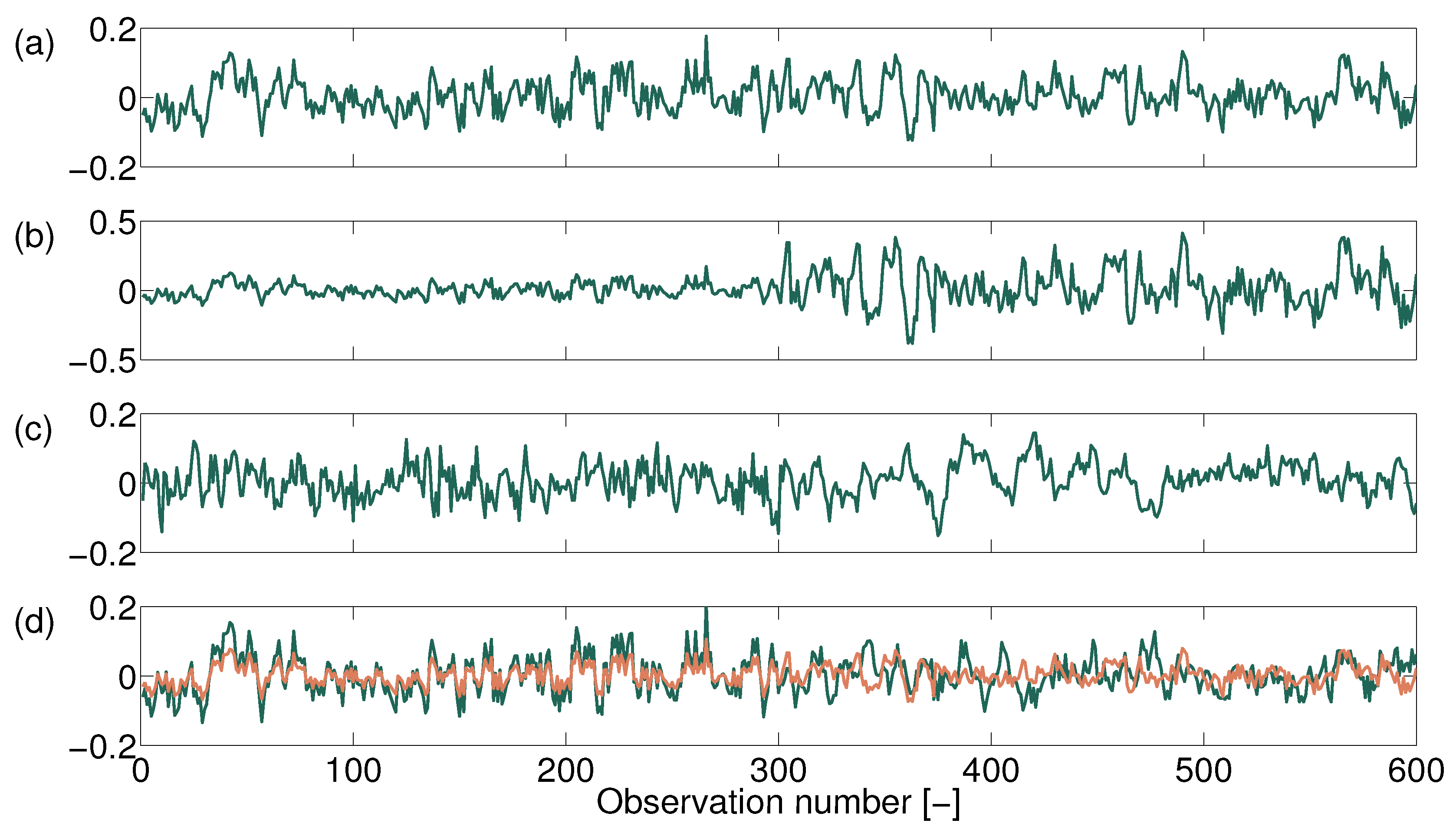
| BFAST anomaly | Anomalies with respect to non-stationary seasonal and trend components. Positive/negative values indicate a higher/lower vegetation greenness (NDVI) than average. |
| 2. Calculation of stability metrics over a 12-year running window | |
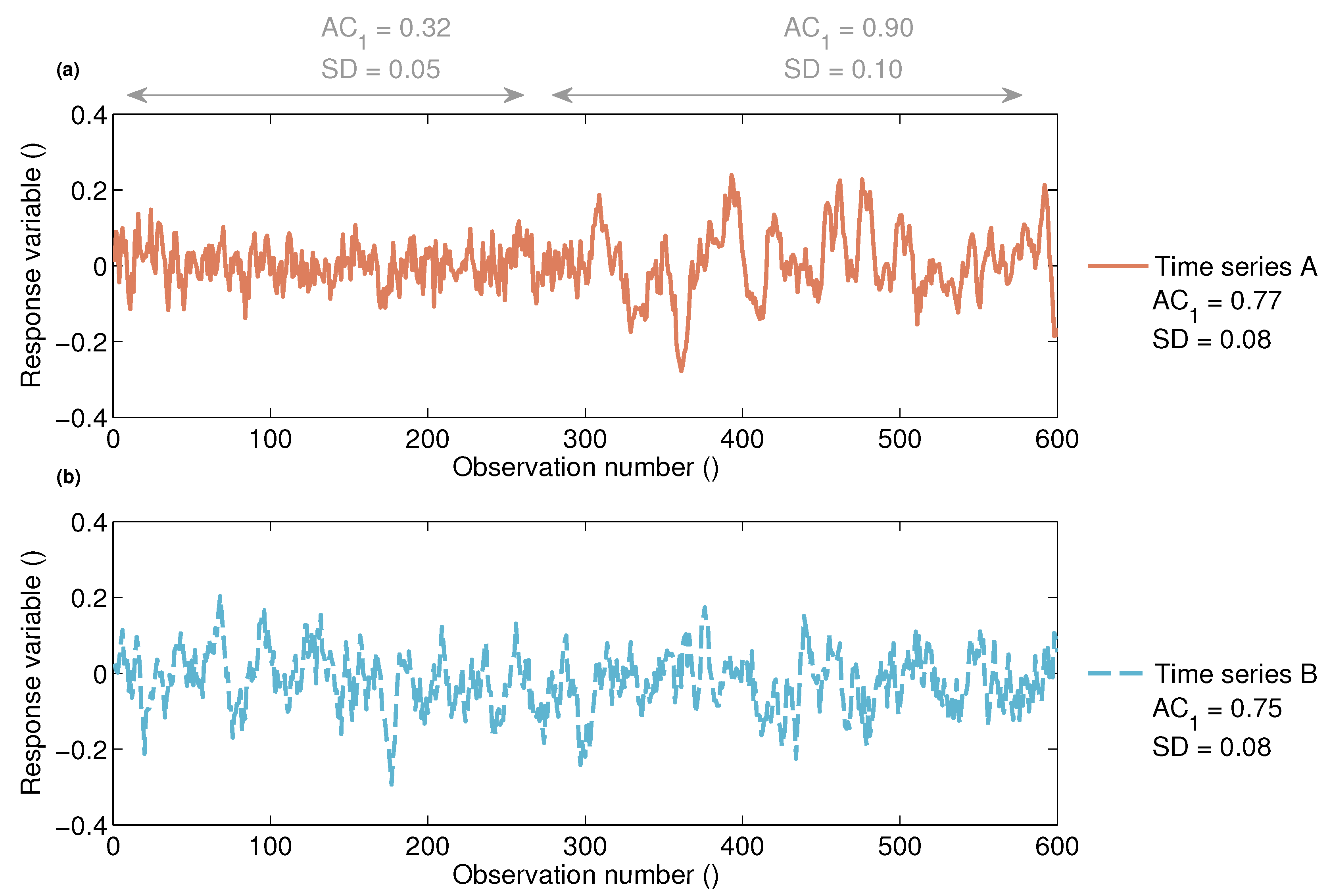
| Standard deviation of the NDVI anomaly (SD) | Indicator of variance. Large/small values denote a large/ small variability. |
| Auto-correlation at lag one of the NDVI anomaly (AC) | Indicator of resilience (memory effect of the biomass response). Large absolute values of the auto-correlation indicate a large memory effect, i.e., a slow return to equilibrium or low resilience. For a positive auto-correlation, the anomalies are similar to the previous anomaly, whereas for a negative value, the anomalies are similar to the previous anomaly, but with the opposite sign. |
| Correlation NDVI anomaly: SPEI (CS) | Indicator related to resistance (immediate response of the vegetation greenness to drought). Large absolute values denote a low resistance, and positive/negative values indicate that a higher greenness than average is associated with a higher/lower water availability than average. |
| 3. Quantification of non-stationarity metrics | |
| Range of stability metric time series | Magnitude of stability metric change. The larger the range, the more the extremes of the stability metric deviate over time. |
| Slope of stability metric time series | Direction of stability metric change. Positive/negative slopes indicate that the metric overall increases/decreases over time. |
© 2017 by the authors; licensee MDPI, Basel, Switzerland. This article is an open access article distributed under the terms and conditions of the Creative Commons Attribution (CC-BY) license (http://creativecommons.org/licenses/by/4.0/).
Share and Cite
De Keersmaecker, W.; Lhermitte, S.; Hill, M.J.; Tits, L.; Coppin, P.; Somers, B. Assessment of Regional Vegetation Response to Climate Anomalies: A Case Study for Australia Using GIMMS NDVI Time Series between 1982 and 2006. Remote Sens. 2017, 9, 34. https://doi.org/10.3390/rs9010034
De Keersmaecker W, Lhermitte S, Hill MJ, Tits L, Coppin P, Somers B. Assessment of Regional Vegetation Response to Climate Anomalies: A Case Study for Australia Using GIMMS NDVI Time Series between 1982 and 2006. Remote Sensing. 2017; 9(1):34. https://doi.org/10.3390/rs9010034
Chicago/Turabian StyleDe Keersmaecker, Wanda, Stef Lhermitte, Michael J. Hill, Laurent Tits, Pol Coppin, and Ben Somers. 2017. "Assessment of Regional Vegetation Response to Climate Anomalies: A Case Study for Australia Using GIMMS NDVI Time Series between 1982 and 2006" Remote Sensing 9, no. 1: 34. https://doi.org/10.3390/rs9010034
APA StyleDe Keersmaecker, W., Lhermitte, S., Hill, M. J., Tits, L., Coppin, P., & Somers, B. (2017). Assessment of Regional Vegetation Response to Climate Anomalies: A Case Study for Australia Using GIMMS NDVI Time Series between 1982 and 2006. Remote Sensing, 9(1), 34. https://doi.org/10.3390/rs9010034