1. Introduction
1.1. Invasive Species in the Desert
Buffelgrass (
Cenchrus ciliaris syn.
Pennisetum ciliare) is a tall, deep-rooted, perennial C4 bunchgrass native to Africa, the Middle East, Asia, and Europe [
1]. It is one of many non-indigenous plant species that were deliberately introduced to North America to beautify, stabilize, or otherwise “improve” natural landscapes, only to demonstrate a competitive superiority that has led to their broad-scale ecological domination. The resulting disruption of ecosystem structure and functioning by individual exotics has had costly and often irreversibly damaging environmental impacts across the United States [
2,
3]. Even the harsh climatic conditions of the semi-arid Southwest do not exempt these lands from biological invasion: some 235 non-indigenous plant species have naturalized in the binational (Mexico/U.S.) Sonoran Desert alone, 62 of which pose a potential or realized threat to the ecological integrity of the desert landscape [
4,
5]. Buffelgrass is one of the most alarming new colonizers of this ecosystem, since it both promotes and benefits from an increase in wildfire intensity and frequency [
6,
7,
8] that can have disastrous ecological consequences: recurrent wildfire events could potentially transform these iconic, species-rich, non-fire-adapted desert environments into monotypic grasslands [
9,
10]. Buffelgrass not only outcompetes other native plants for scarce resources [
11,
12] but it fills in the interstitial gaps between cacti and shrubs, creating a continuous mat of fine fuels [
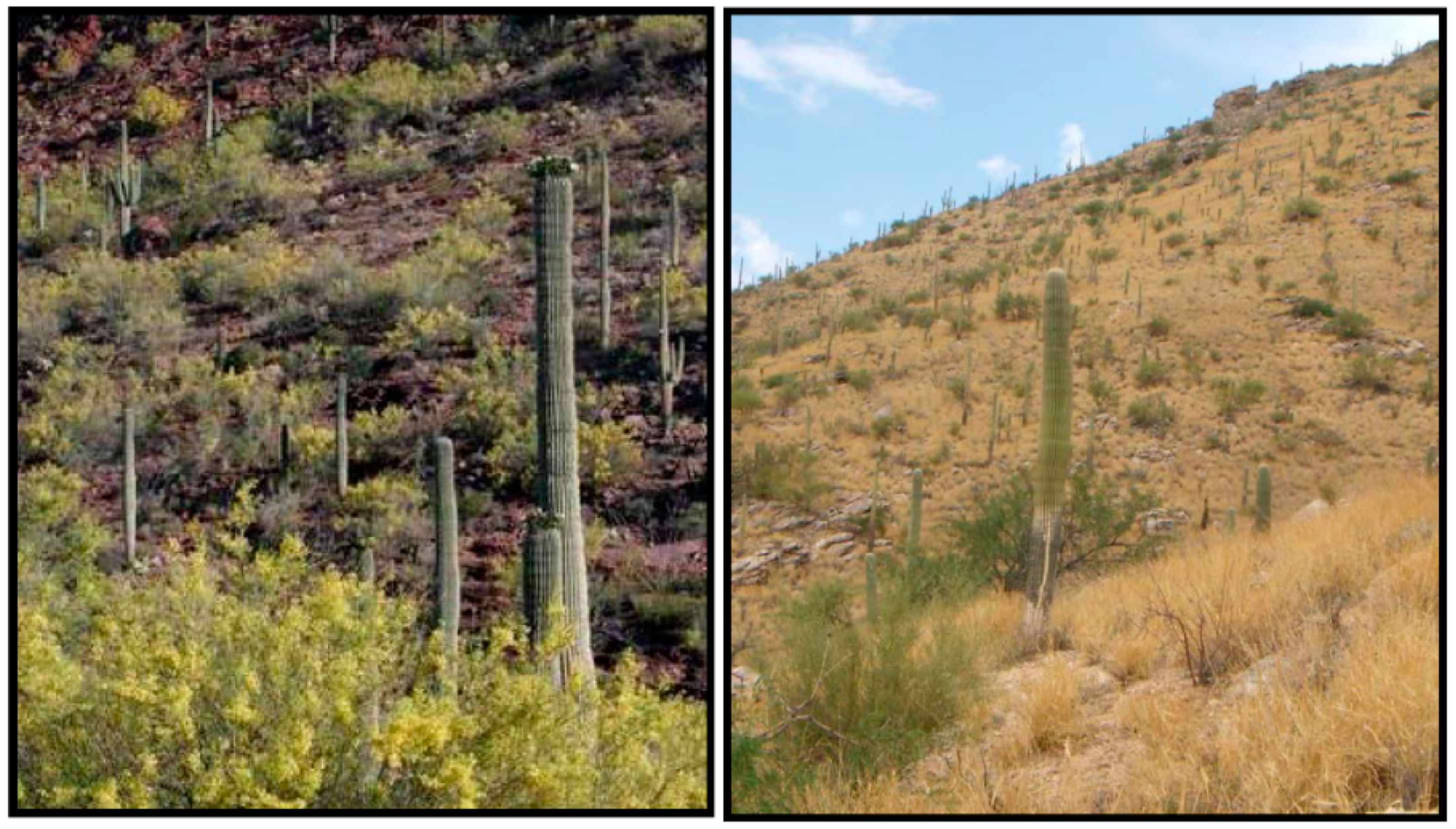
13] that lead to structural changes across the landscape (
Figure 1).
1.2. Buffelgrass in Saguaro National Park
The potential for buffelgrass to fundamentally alter the structure and functioning of dryland ecosystems [
9,
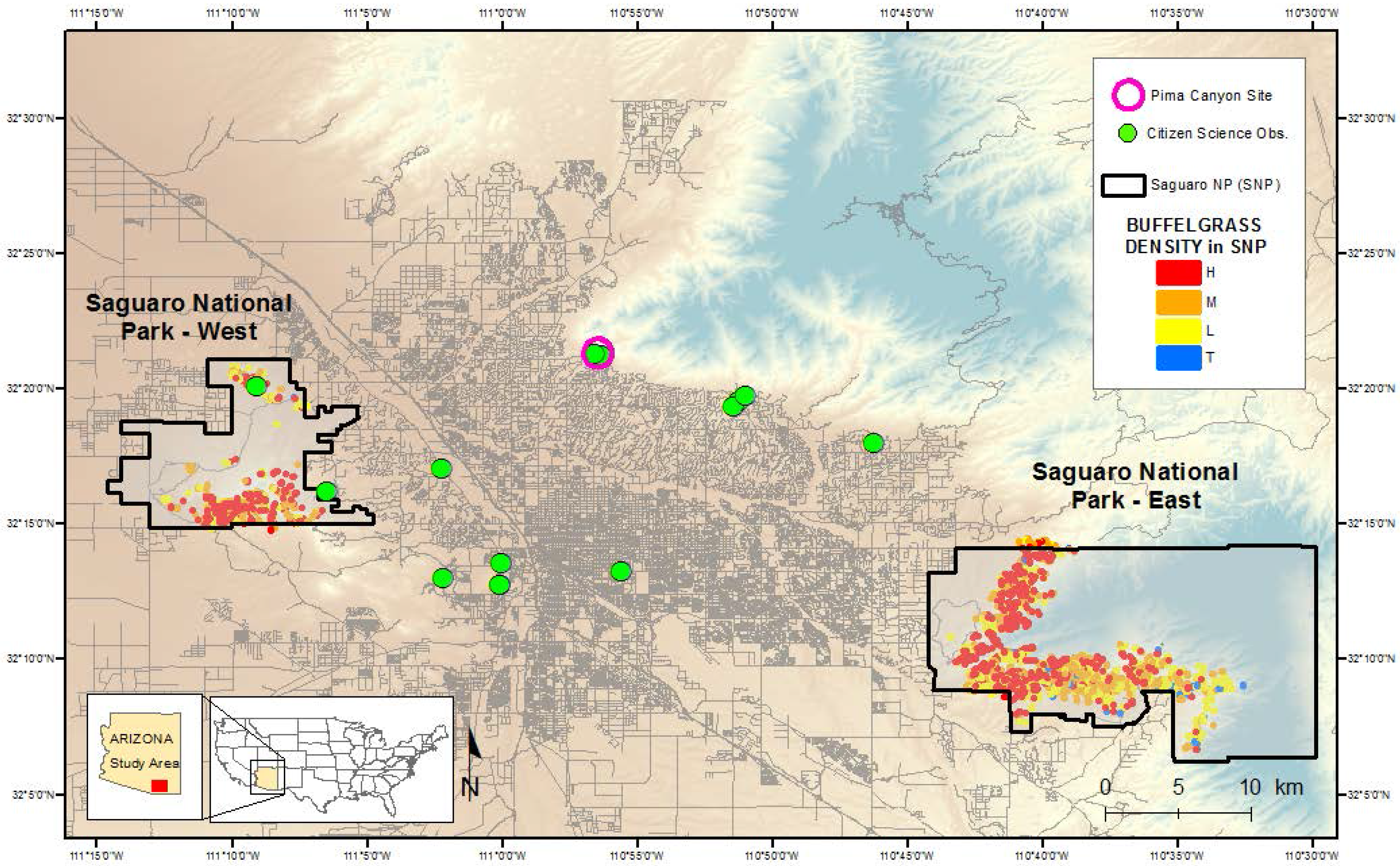
14] makes it singularly unwelcome in areas prized for their archetypal Sonoran Desert landscapes, such as Saguaro National Park (SNP) in Southern Arizona (
Figure 2). Buffelgrass was first observed in SNP in 1989; within 20 years the invasive grass covered an estimated 800 hectares, despite the mobilization of substantial park and volunteer resources to manually remove plants [
15]. The most recent estimates of the buffelgrass extent are 2000 acres [
16]. SNP managers consider the complete eradication of buffelgrass in the park to be effectively impossible, but aggressively work to constrain further encroachment given the plant’s destructive potential [
17]. Infestations in rugged, remote areas of SNP that cannot be readily reached by field crews are treated with aerial applications of herbicide. The timing of application is critical since the herbicide is most effective while the plant is actively growing and is at least 50% green. However, the appropriate timing can be difficult to determine given the heterogeneity of the landscape and variability of monsoon-driven greenness in the region. For example, in 2015 aerial spraying in SNP’s western Tucson Mountain District was cancelled because the buffelgrass in that area had already entered dormancy [
18]. To minimize the impact on surrounding native vegetation and ensure the optimal effectiveness of herbicide applications, park managers need to know not only where outlying buffelgrass patches are, but when they are most photosynthetically active.
1.3. Using Phenology and Remote Sensing to Map Invasive Grasses
Remote sensing data could provide a practical and economical alternative to field-based methods for locating and monitoring buffelgrass infestations in remote areas of SNP, provided that the imagery shows both the presence and phenological status of the plants. Images collected via aircraft or unmanned aerial vehicles allow for fine-scale visual differentiation of vegetation types; researchers have tracked the spread of buffelgrass in the foothills of the Tucson mountains by identifying individual plants on high-resolution (sub 1-m pixel size) aerial imagery collected at irregular intervals over a 21-year period [
19]. The phenological development stage, however, can only be determined from an imagery collection rate that is unfeasible with aerial campaigns given the economic limitations of most natural resource budgets.
Time series of Landsat Thematic Mapper (TM)/Enhanced Thematic Mapper Plus (ETM+) and Moderate Resolution Imaging Spectroradiometer (MODIS) data are an attractive alternative due to their frequent acquisition (daily to every 16 days), synoptic collection extent, the suitability of the imagery for vegetative analysis purposes, and the free accessibility of current and archived data. Since the coarse spatial resolution of each pixel (>900 m
2) confounds the identification of individual plants based on spectral or morphological characteristics, remote sensing-based studies of invasive grasses in the western U.S. have typically exploited asynchronous green-up patterns of native and non-native grasses (
i.e., phenology [
20]) to detect infestation patterns when using these data.
Bradley and Mustard [
21] took advantage of the amplified interannual response of invasive cheatgrass (
Bromus tectorum) to rainfall to map infestations across the Great Basin watershed using Landsat and Advanced Very High Resolution Radiometer (AVHRR) data. Peterson [
22] estimated and mapped percent cheatgrass ground cover in Nevada on the basis of the invasive species’ relatively early spring green-up and subsequent senescence, which were identifiable from two Landsat ETM+ images. Singh and Glenn [
23] also relied on the phenological distinctiveness of cheatgrass to classify its distribution in Idaho; their approach applied hyperspectral processing techniques to a temporal stack of Landsat scenes assembled over a single growing season. Another invasive grass, Lehmann’s lovegrass (
Eragrostis lehmanniana) was successfully mapped on the basis of 250 m MODIS data by Huang and Geiger [
24] and Huang
et al. [
25], who exploited the tendency of the plant to produce higher amounts of biomass under wet conditions in cool seasons, when the native vegetation was still dormant.
Like many Sonoran Desert native grasses, buffelgrass principally relies on warm-season monsoon precipitation for growth [
26,
27]. However, the invasive responds more quickly to moisture inputs than native grasses [
28,
29,
30], resulting in an accelerated germination of new plant material after rainfall events. The response of one buffelgrass plant observed for this study to the 2014 monsoon is shown in the
supplementary file. Our study investigates the hypothesis that this precipitous growth can be leveraged to identify buffelgrass locations and determine when the plants are most photosynthetically active.
1.4. Objective
Our research objective is to detect when and where invasive buffelgrass is photosynthetically active in the Tucson, Arizona region. To effectively manage buffelgrass, National Park Service (NPS) land managers at Saguaro National Park need to know not only the distribution of the invasive grass across the landscape but also its phenological status, since the herbicide is most effective if applied when the plants are at least 50 percent green. If such knowledge can be provided in an operational and timely manner, land managers can optimize treatment activities. Managers particularly need to be able to map, monitor, and treat buffelgrass in remote areas. This research, therefore, explored the dynamics between buffelgrass condition on the ground and synoptic measures of landscape and climate with the goal of mapping when and where buffelgrass is green.
2. Location and Datasets
2.1. Study Site
The study location comprises the east and west districts of 37,006 ha Saguaro National Park, which borders the city of Tucson, Arizona, in the southwestern USA (
Figure 2). The Sonoran Desert climate is characterized by hot, dry summers and temperate winters. Precipitation in the Southern Arizona study area averages 300 mm annually, and occurs primarily in a bimodal distribution: a cool-season period (December–February) and a hot summer monsoonal period (July–September). On average, the two periods receive approximately equal amounts of precipitation ([
31]). The Southwest ReGAP vegetation ecosystem type Sonoran Paloverde-Mixed Cacti Desert Scrub predominates, with a sparse to moderately dense canopy of xeromorphic deciduous and evergreen tall shrubs, and various cacti species, including the signature saguaro (
Carnegia gigantea) for which the park is named [
32].
2.2. Satellite Data
To compile landscape-wide indications of vegetation greenness, we downloaded all available 8-day composite Moderate-resolution Imaging Spectroradiometer (MODIS) reflectance images (46 per year) for 2011, 2012, and 2013 from [
33]. MODIS products are compiled at a range of spatial resolutions; we accessed the highest resolution dataset (250 m; available as product MOD09Q1) given our goal of distinguishing the smallest possible patches of buffelgrass across the landscape. The composite dataset is produced by selecting the pixel obtained during the eight-day period that contains the best possible observation as evaluated on the basis of favorable coverage and view angle, the absence of cloud contamination, and aerosol loading [
34], resulting in data that are pre-filtered for quality. We retrieved MODIS bands 1 (red; 620–670 nm) and 2 (near infrared (NIR); 841–876 nm); pre-processing of the data included reprojection to UTM zone 12 using nearest neighbor techniques. We created Normalized Difference Vegetation Index (NDVI) images from the normalized ratio of the near-infrared (NIR) and red bands. Vegetation exhibits a distinctive spectral reflectance pattern, with low reflectance of red wavelengths due to chlorophyll absorption and strong reflectance in the near-infrared (NIR) due to cellular structure. The NDVI exploits this distinctive signature to provide a measure of the photosynthetic activity of plants. All image processing was performed in ERDAS Imagine (v. 10.0) (Stockholm, Sweden).
2.3. Citizen Science Observations-Pima Canyon
We accessed a record of high-frequency buffelgrass observations taken at a single location near Tucson (in lower Pima Canyon) for this study. Pima Canyon is located in the Santa Catalina foothills on the northern edge of the city (
Figure 2) in geomorphic conditions similar to those of Saguaro National Park–East;
i.e., mountainous terrain composed of felsic granitic and metamorphic rocks. The south-facing slope of the Santa Catalina Mountains, which includes the Pima Canyon area, has a particularly dense and widespread buffelgrass infestation [
19]. The observations were collected by a single observer (co-author Weltzin) on a near-weekly basis from July 2010 to December 2014 using standardized protocols [
35]; data were archived in the USA National Phenology Network (USA-NPN) database [
36]). The visual estimates of percent greenness of up to five individual buffelgrass plants located along a south-facing slope of the trail were assessed on each day of observation (
Figure 2). The number of plants varied over the period of observation because plants were occasionally removed during buffelgrass management events. Nonetheless, it was always possible to find alternate plants nearby to include as substitutes. For this study, the greenness values of all the individual plants observed on a single day were averaged and assigned to the coincident eight-day composite MODIS interval (1 to 46 in each year). If observations were conducted on more than one day during an eight-day interval, the daily values were averaged. If no observation occurred within a composite interval, greenness estimates from the two bracketing time periods were averaged and assigned to that interval. If observations were absent for more than one consecutive interval, they were considered “no data” values.
2.4. Citizen Science Observations-Tucson
Beginning in June 2013, we recruited 10 citizen scientist volunteers to participate in the USA-NPN project Nature’s Notebook [
37] Citizen and Professional Science project for buffelgrass observations in the Tucson region (
Figure 2). The volunteers were trained through the USA-NPN Education Coordinator and the Southern Arizona Buffelgrass Coordination Center (SABCC) as part of an effort to engage the general public in long-term phenology monitoring. Those interested in collecting data were encouraged to select a buffelgrass patch or individual plant to follow. All proposed locations were field checked and characterized by co-author Patrick-Birdwell, and on-site training was provided. As at the Pima Canyon site, observations followed a series of strict protocols designed to capture detailed information regarding the timing and proportion of plant green-up, flowering, fruiting, and senescence ([
35]). More information about the project can be found on the USA-NPN Tucson Phenology Trail website ([
38]); data are available from the USA-NPN database ([
39]). By the end of 2014, 6913 observation records and 896 site visits had been entered into the database by the volunteer participants. The broad geographical distribution of these observations provided a complementary dataset to the single-site, long-term records from Pima Canyon.
2.5. Map of Buffelgrass Extent and Density
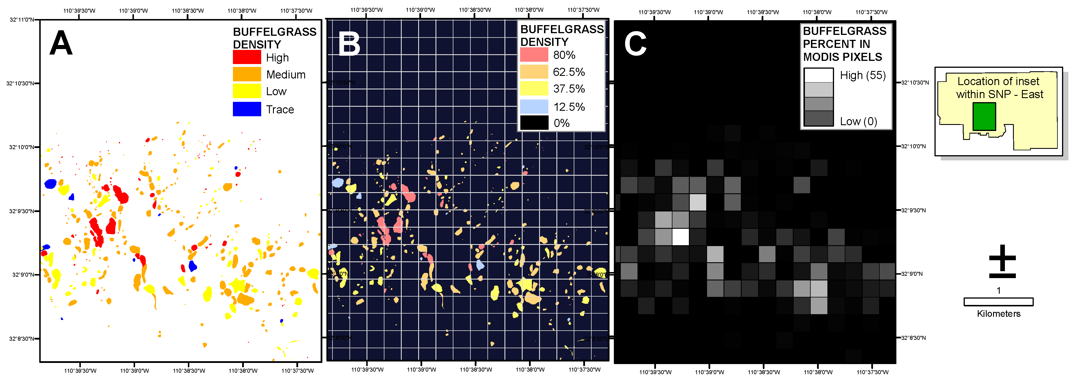
The National Park Service supplied a map of buffelgrass locations and densities within both SNP districts produced from a September 2012 helicopter survey conducted to document the distribution and quantity of buffelgrass, estimate its growth and spread, and prioritize areas for treatment. The overflight was timed to coincide with a period when buffelgrass was senesced and visually distinct from surrounding native vegetation. Observers used a GPS-based digital aerial sketch mapping (DASM) system developed by the United States Forest Service (USFS) Remote Sensing Applications Center (RSAC) and USFS Forest Health Technology Enterprise Team to delineate the areas of buffelgrass extent. Each area was tagged with a visual description of the assessed buffelgrass density: trace (1% to 25%), low (>25% to 50%), medium (>50% to 75%), or high (>75% to 100%). To transform the polygonal coverages to the raster-based format of the remote sensing data, we calculated the percent of buffelgrass within each MODIS pixel by assigning the midpoint value to each polygon for low to medium density values (
i.e., 12.5%, 37.5% and 62.5% for trace, low and medium respectively) and 80% to the high density category. We then converted the polygon coverage to a 5-m raster attributed with the percent values, and averaged all pixel values within each MODIS footprint (
Figure 3).
2.6. Precipitation Data
Two different sources of rainfall data were used for analyses conducted at a single site (Pima Canyon) and those conducted over a landscape extent (SNP East and West). For Pima Canyon we accessed the closest source of recorded precipitation information, which was MesoWest daily data ([
40]) at station AT021 (32.33050°N, 110.9120°W). The station is within 4 km and at a similar elevation (890 m) as the observation site. For the landscape comparison, we downloaded PRISM (“Parameter-elevation Regressions on Independent Slopes Model”) daily rainfall data ([
41]) over the SNP districts. Using nearest neighbor techniques, we resampled the 4 km PRISM data to 250 m to conform to the spatial resolution of the MODIS data. This technique replicates data across the extent of the resampled pixel (
i.e., each 4 km pixel yields 256 (16 × 16) 250 m pixels, each with the same value), but enables the direct comparison of NDVI and precipitation data over broad geographical areas. For both datasets, we summed daily precipitation values over eight-day intervals to coincide with the MODIS composite data. The PRISM data used in this study includes a year with an exceptionally wet monsoon (2011) and an exceptionally dry monsoon (2013). Average monsoon rainfall is 154 mm (6.08 in); monsoon totals for 2011, 2012 and 2013 were 219 mm (8.62 in), 153 mm (6.02 in) and 95 mm (3.74 in), respectively ([
42]). The study time period thus encompassed years with relatively wet, average, and distinctly below-average monsoon precipitation totals.
3. Methods
3.1. Overview and Exploratory Analyses
Relationships between field-observed greenness, MODIS satellite greenness and precipitation data were explored and characterized at the Pima Canyon site, given the temporal depth of these data. Simple linear regression analyses and Spearman’s correlation coefficients were used to quantify relationships among the variables. Initially, MODIS data at daily, 8-day composite and 16-day composite intervals were compiled and examined. We also examined both NDVI, which is the most common vegetation index used, and the Enhanced Vegetation Index (EVI), which minimizes soil background variations and includes corrections for atmospheric contamination using blue band reflectance.
It became apparent early in our research that daily MODIS data were too noisy to yield an operational product, so they were removed from consideration. The EVI was only available as a product with 16-day MODIS composite data, and since these composites are only produced every 16 days, their application as an input to an operational process was limited. Early linear regression results were comparable using EVI and NDVI data, which is reasonable since this study looked at the dynamics of greenness; the substrate remains constant at each location and is thereby effectively normalized. Furthermore, given that NDVI is calculated using two commonly collected reflectance bands (red and near-infrared) and can be easily derived from many sensors, we considered it more likely to be generalizable and transferrable. It also became apparent that an approximate weekly time-step made sense for providing information to guide land management actions. We therefore chose to use MODIS 8-day composite reflectance data for this study, from which we calculated the NDVI. Many early analyses were conducted using MODIS 16-day EVI data; some of these results are shared in the Discussion Section and reported in our appendices.
Relationships identified and quantified at the Pima Canyon site were used to derive predictive metrics for the distribution of buffelgrass in SNP. The ability of the metrics to identify locations of known buffelgrass was tested by using the 2012 SNP buffelgrass mapping results as validation. The predictive relationships were also examined using data from the other citizen science sites, confirming the correlations, although an exceptionally dry monsoon in 2013 delayed analyses with these locations until the full spectrum of greenness conditions were realized in the landscape after the 2014 monsoon season.
Data from all citizen scientist sites and Pima Canyon were used to establish relationships for predicting buffelgrass phenological status, i.e., to predict when buffelgrass would be green enough to successfully treat with herbicide.
3.2. Precipitation and Vegetation Greenness Correlations at Pima Canyon Citizen Science Site
The Pima Canyon data were analyzed separately for this study objective because of the frequency, consistency, and extended period of the observations. To evaluate the relationship between observed citizen science and satellite-derived greenness, we calculated Spearman’s correlation coefficients between the direct observations of percent greenness collected and current and lagged MODIS NDVI values for each year from 2010 to 2013. The precise location of the plants observed and averaged for this site straddled the boundary between two 250-m square MODIS pixels. The northern-most pixel contained the majority of the plants monitored and was most representative of the imaged landscape, since a heavily-vegetated desert wash intersected the southern boundary of the southern MODIS pixel. NDVI data were therefore extracted from the northern MODIS pixel. To evaluate the relationship between buffelgrass green-up and precipitation, we calculated correlation coefficients between field measurements of percent greenness and current and lagged measures of precipitation from the neighboring weather station (MesoWest AT021) over the same time period. These correlations established the relationships between the single-site buffelgrass and precipitation data.
3.3. Precipitation and Vegetation Greenness Correlations at Saguaro National Park (SNP)
On the basis of the correlations determined at the Pima Canyon site, we created a novel suite of metrics (“Climate Landscape Response” (CLaRe) metrics) to predict buffelgrass locations in SNP from park-wide satellite NDVI measurements and gridded 4 km precipitation data. These metrics range from 0 to 1.0 and quantify the strength of the linear relationship between the satellite greenness value and various cumulative precipitation values. They are created by conducting a linear regression between the NDVI and a precipitation value at each pixel and extracting the correlation coefficient. Since we wanted to use the 2012 helicopter mapping as validation, we restricted the calculation of metrics to the 2011–2013 time frame, thereby bracketing the year the “ground truth” mapping data were generated. Statistical tests, including Student’s t-tests, were conducted to evaluate if the metrics were effective at separating pixels of pure native vegetation from those with buffelgrass. The CLaRe metrics with a balance between spatial and temporal prediction were used to create models of buffelgrass presence/absence in the park. That is, we used metrics that spatially displayed strong overall correlations and separability, but temporally allowed for earlier prediction of buffelgrass presence and condition. Buffelgrass presence/absence models were validated by examining their spatial coincidence with confirmed buffelgrass locations.
3.4. Predicting Buffelgrass Greenness
The linear regression analyses with strong (>0.50) correlations between greenness observed on the ground and various cumulative and lagged precipitation values were solved for the desired 50 percent greenness condition, which is the minimum greenness for which herbicide application can be effective at killing the invasive grass.
4. Results
4.1. Pima Canyon
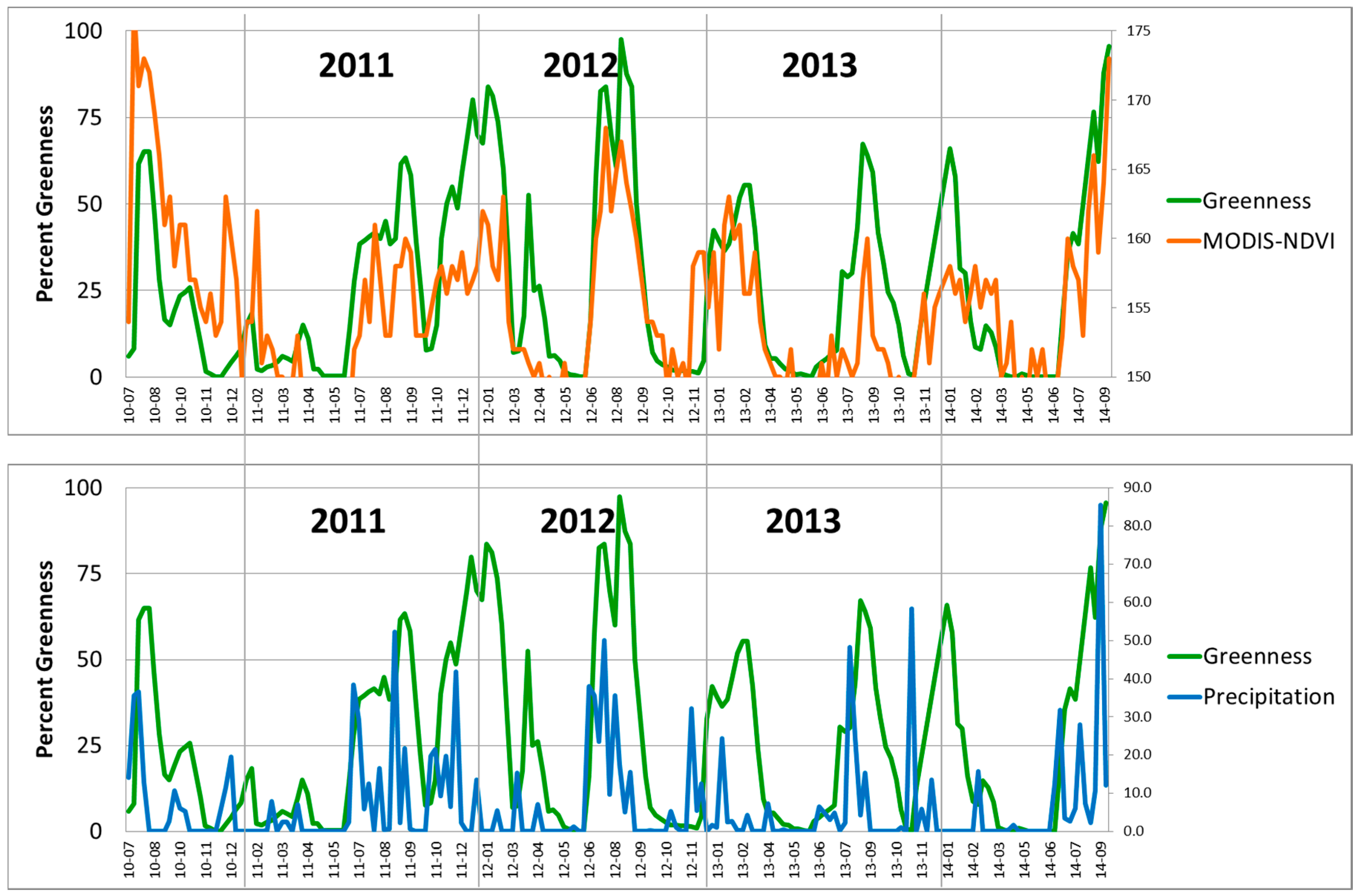
Strong relationships exist at Pima Canyon between buffelgrass greenness observed on the ground and both MODIS greenness and PRISM precipitation. These relationships are visually evident in
Figure 4, which plots the variables compiled for eight-day intervals and uses MODIS NDVI greenness. In particular, the field observations of buffelgrass greenness and those extracted from MODIS data are temporally synchronous, while buffelgrass greenness distinctly lags precipitation events.
We quantified the strength of the relationships between field-observed greenness and various combinations of current and lagged 8-day MODIS NDVI and precipitation using linear correlation analysis.
Table 1 summarizes the correlation coefficients between a subset of the relationships tested, showing field measurements of buffelgrass greenness are highly correlated with MODIS greenness from the coincident 8-day time period, and are highly correlated with precipitation totals of prior time periods. We also see strong correlation between MODIS greenness and the same lagged precipitation totals, a result which follows given that field greenness correlates to both MODIS and lagged precipitation.
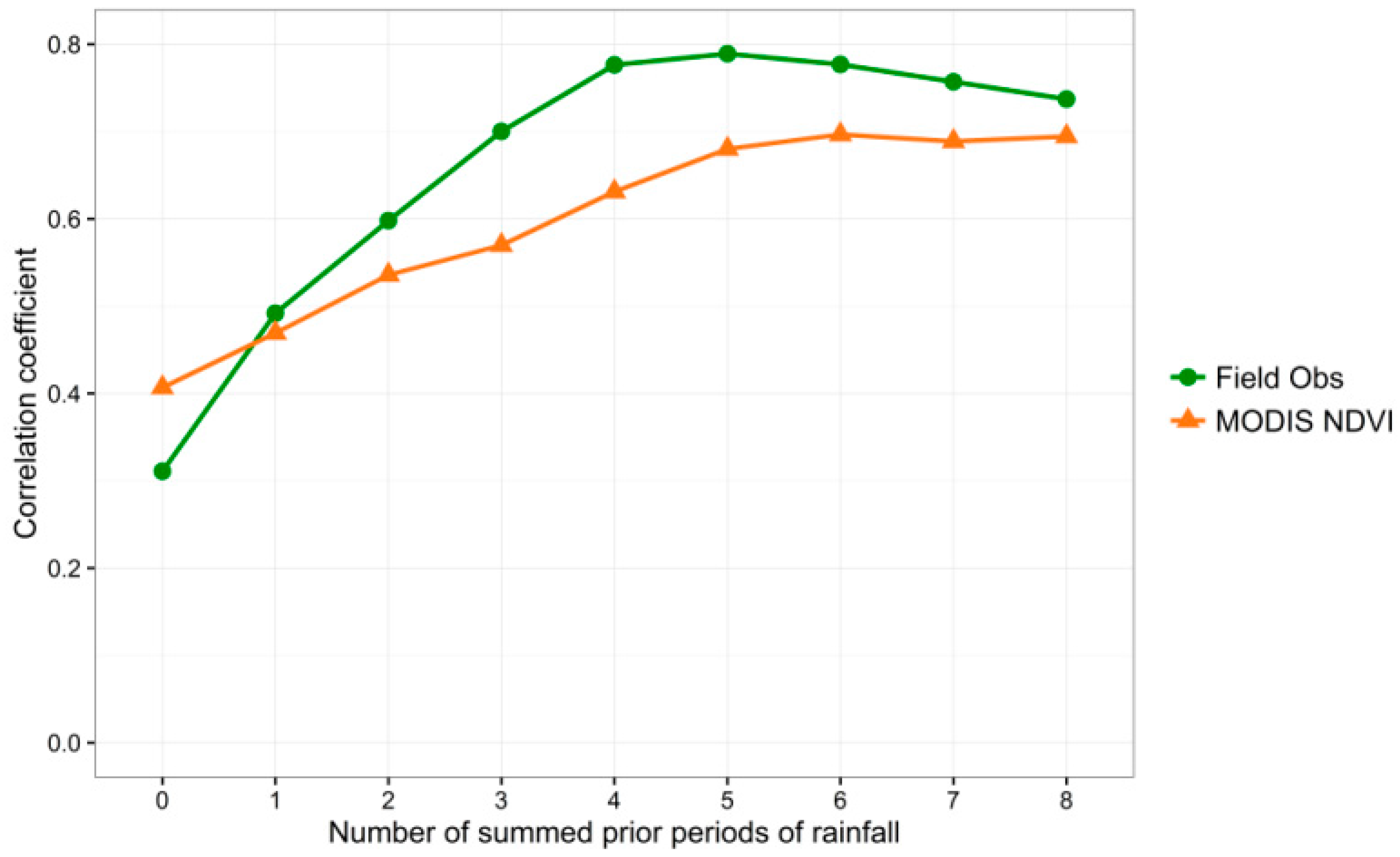
Figure 5 explores these relationships at Pima Canyon further, and graphs the correlation coefficients for the linear relationships between a sequence of cumulative precipitation values and both eight-day MODIS NDVI values and field observed greenness values, revealing strong (>0.5) correlation for all cumulative precipitation totals except the current (ppt0) and the prior time period (ppt1). Note the maximum correlation for field observed greenness of nearly 0.8 occurs at the cumulative lagged precipitation from the prior five time periods (ppt12345), with longer-term correlations dropping slightly from there. The MODIS correlations level off above ppt12345. For this study, we chose a maximum lag of 8, corresponding to approximately two months, due to this observed drop-off at the buffelgrass-rich Pima Canyon site and because we considered two months a desirable maximum time frame for land management planning.
4.2. Saguaro National Park (SNP)
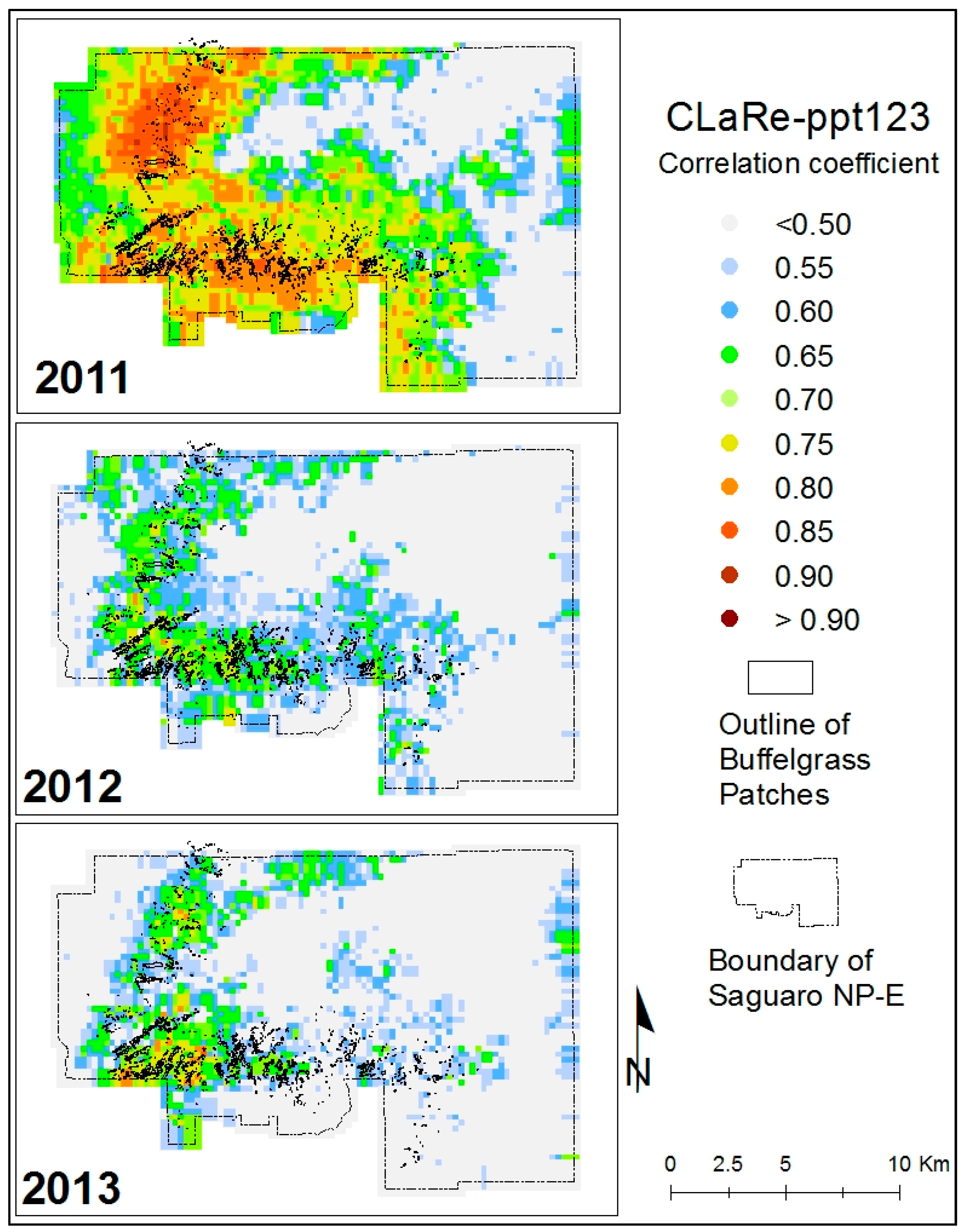
Several CLaRe metrics were developed from correlations quantified at the Pima Canyon site and mapped across the SNP study area. These metrics capture the strength of the relationships between satellite-measured greenness and various lagged precipitation values. At each pixel for each year, the correlation coefficient describing the strength of the linear relationship between the 46 MODIS NDVI values and the cumulative precipitation for time periods of different lags was calculated. For example, the correlation between MODIS greenness and the cumulative precipitation for the prior three eight-day periods (ppt123) for 2011, 2012 and 2013 is shown in
Figure 6. Overlaid on these figures are the polygons of buffelgrass mapped in 2012 via the helicopter survey. We observed an especially strong spatial coincidence of the buffelgrass patches and the high correlation values for all years using this CLaRe metric.
Given the results at Pima Canyon, which contains abundant buffelgrass, and knowing that buffelgrass can break dormancy to respond to water faster than native plants [
28], we anticipated that areas with buffelgrass might exhibit stronger precipitation-greenness relationships than areas without. Our results confirmed this, showing that the presence of buffelgrass is indeed captured by the CLaRe metrics, including CLaRe-ppt123 displayed in
Figure 6. Of particular note is that the
pattern of high CLaRe values is the same in all three years, even though the climate varied, with 2011, 2012 and 2013 years of above, normal and below average monsoon precipitation, respectively.
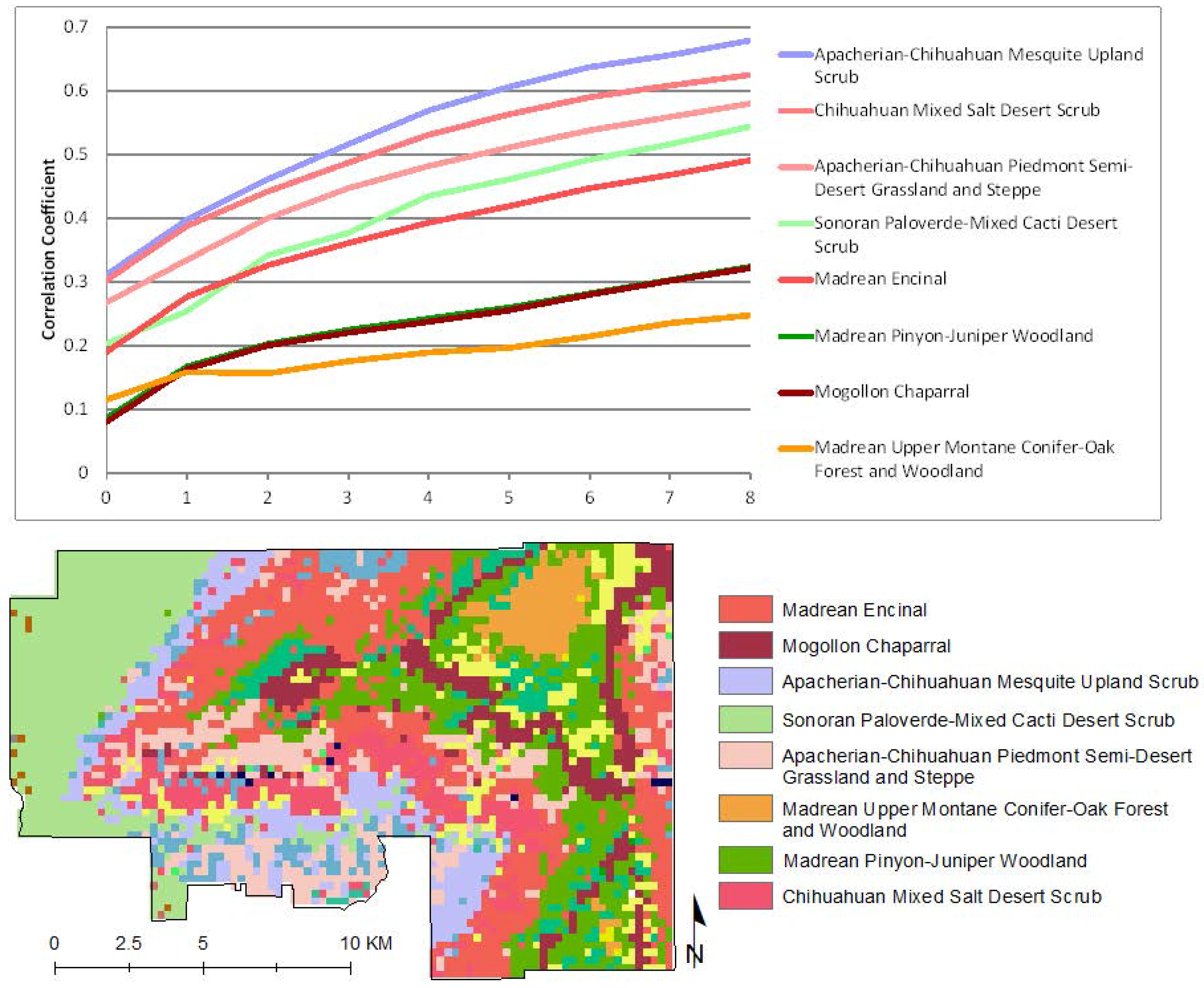
To explore the response of native vegetation communities to precipitation, we isolated all pixels that had had no buffelgrass mapped in the 2012 aerial helicopter survey, and stratified them according to the major vegetation classes in the park; their precipitation/MODIS greenness correlations are presented in
Figure 7. Several patterns are evident. In all cases but one, the native vegetation types show very low correlation to recent precipitation, with values less than 0.5 for current precipitation and up to three eight-day periods of cumulative lagged precipitation. In all cases, correlation strength increases through time, showing that native vegetation types are more increasingly correlated to longer-term cumulative precipitation. In addition, the CLaRe phenometrics effectively stratify the vegetation types by rooting depth, with deep-rooted woodland and forest showing the lowest correlation values and shallower-rooted grasslands and scrublands showing higher correlation.
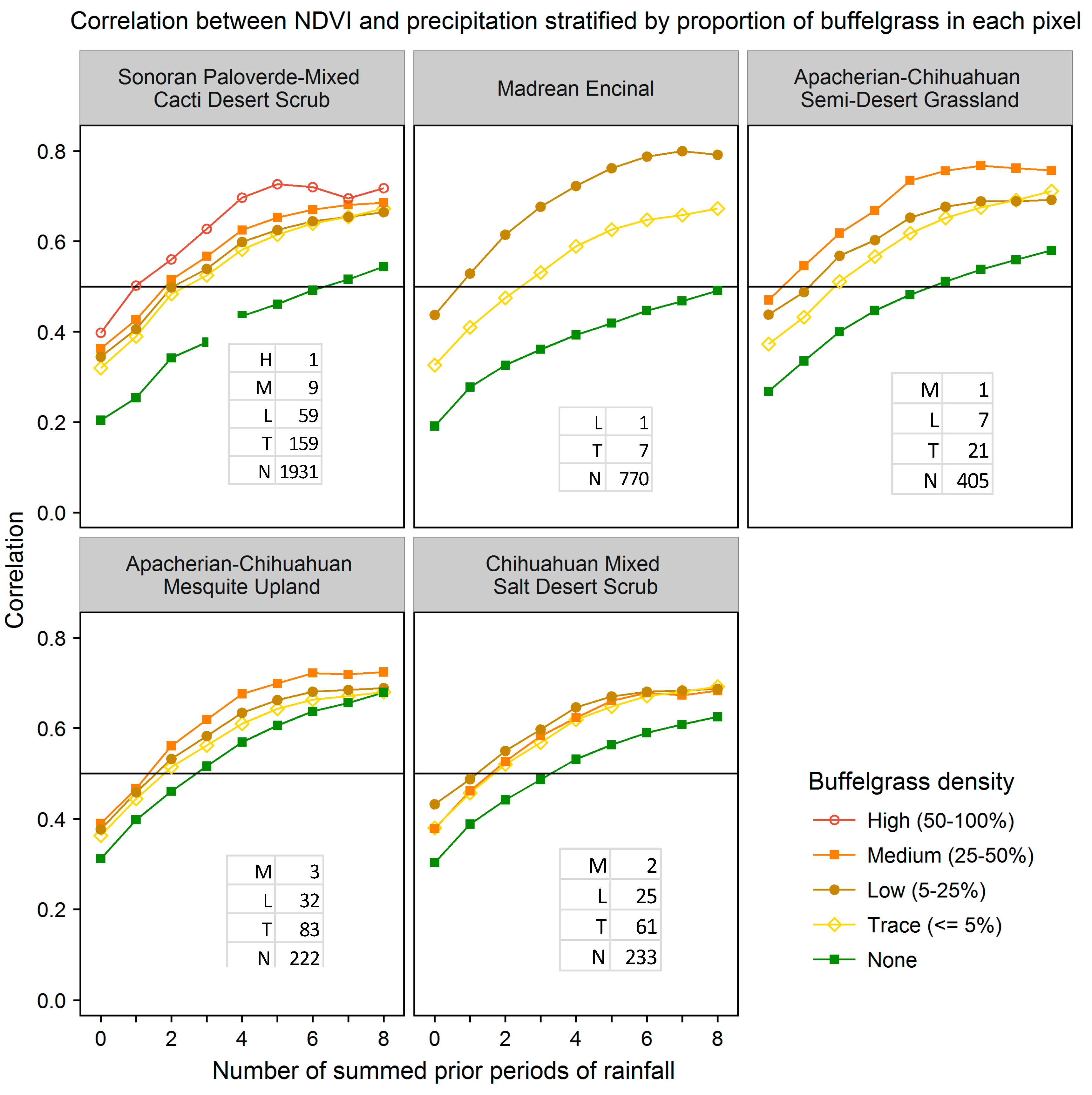
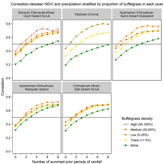
We evaluated the ability of various CLaRe phenometrics to locate buffelgrass by stratifying the landscape first by vegetation type and then by the density of buffelgrass within the pixels (
Figure 8). The map shows the dominant vegetation types in each MODIS pixel footprint as mapped by the Southwest Regional Gap Analysis Project (SWreGAP, [
32]). Full descriptions of these vegetation types can be found at: [
43] Note that even small amounts of invasive buffelgrass in the landscape have a strong effect on the correlation coefficients in the CLaRe phenometrics.
As seen in previous plots, the curves of all pure native vegetation types (the green curves in
Figure 8) are monotonically increasing, whereas several of the curves for high density buffelgrass (the brown curves in
Figure 8) peak and then decrease as the number of lagged time intervals increases. This is the same pattern seen at Pima Canyon (
Figure 5). The buffelgrass curves are distinctly different than the curves for native Sonoran Desert vegetation communities. Not only do they display consistently higher correlations to all variations of cumulative precipitation, revealing that the invasive responds quickly to precipitation, but also these curves often peak, reflecting the invasive’s aggressive growth pattern.
T-tests (
Table 2) reveal there are significant differences between the correlation coefficients for pure native vegetation and buffelgrass-invaded pixels for CLaRe phenometrics across all three years and across all vegetation types in the park, with exceptions in the Apacherian-Chihuahuan mesquite upland scrub vegetation type and in 2013, which experienced an abnormally dry monsoon. The CLaRe correlations are overall weaker in the dry year of 2013 and much stronger in the wet year of 2011. In contrast to the wet year 2011, some of the average correlation values for buffelgrass pixels in 2013 are less than those for native pixels in the dry year.
4.3. Mapping Buffelgrass–Where?
Using the CLaRe metrics and the results for the individual vegetation types, we created several models of buffelgrass presence/absence. For modeling purposes, we focus on SNP-East, given its geologic and geomorphic similarity to the Pima Canyon site and its diversity of vegetation types and elevational gradients. We also focus on the shorter-term cumulative precipitation lags, given that we seek to provide operationally timely data and that these CLaRe metrics display strong differences between pure native and buffelgrass-invaded pixels. Our modeling was conducted by choosing options that seemed logical, useful and easily understood by practitioners; we did not apply statistical methods to optimize classification.
We initially used the observations from 2011 and the three CLaRes ppt12, ppt123 and ppt1234. These were chosen because 2011 was a wet year and statistical tests (
Table 2, left panels) reveal the most significant differences between pure native and buffelgrass-invaded pixels. Each vegetation type was isolated and the mean value observed at buffelgrass-invaded pixels was used as a threshold separating buffelgrass presence/absence (
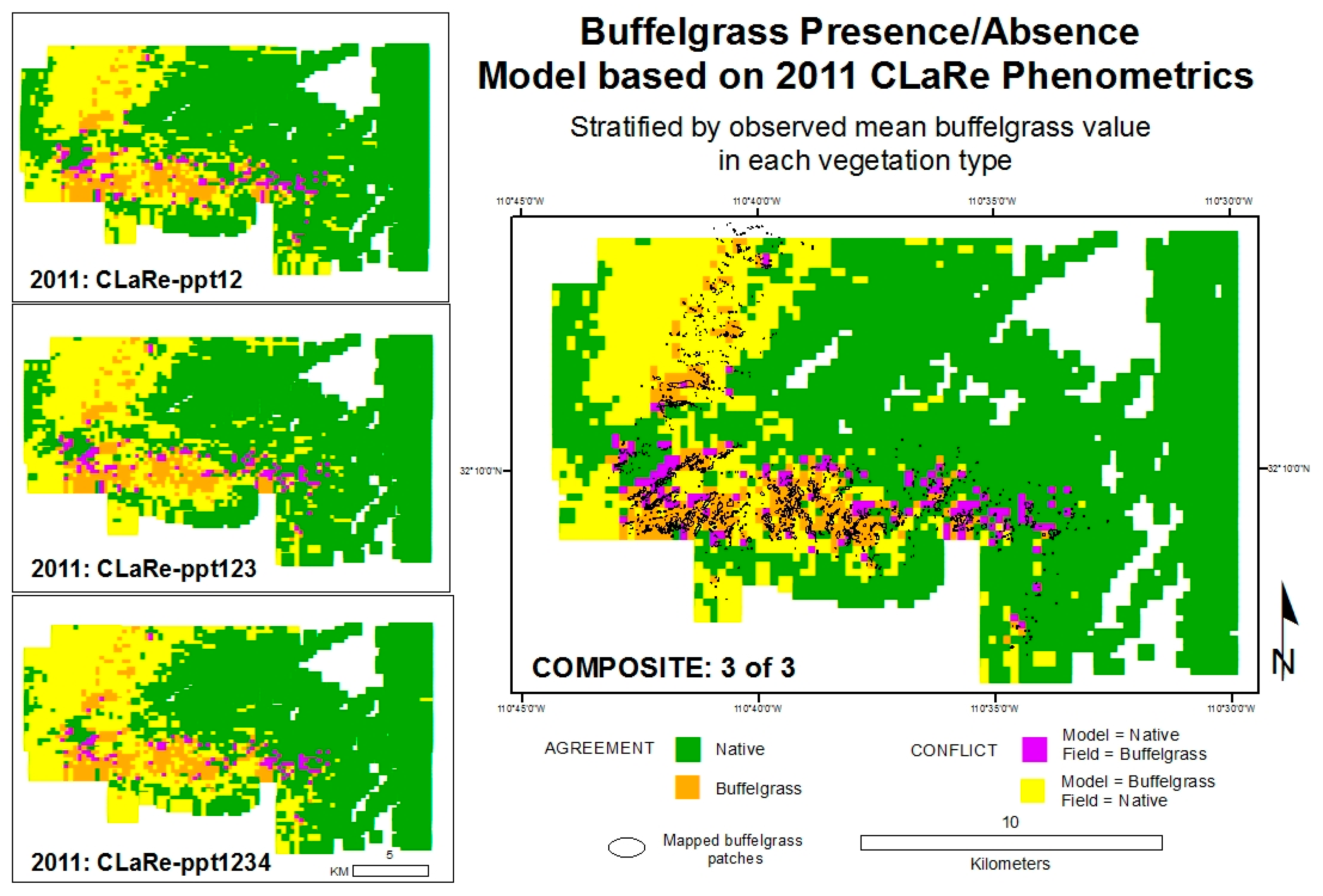
Figure 9, left images). We omitted pixels with buffelgrass density less than 1 percent to amplify the difference between buffelgrass presence/absence. A composite model (
Figure 9, right image) maps buffelgrass presence if all three sub-models (ppt12, ppt123, ppt1234) identified a given pixel as containing buffelgrass. The models were validated by seeing how well they predicted the mapped buffelgrass polygons, using the derived raster of percent buffelgrass in MODIS pixels as reference data. The overall accuracies of the sub-models range from 70 to 74 percent, with 60 to 65 percent of known buffelgrass patches accurately mapped, but with high errors of commission (
i.e., many pixels of native vegetation are misclassified as buffelgrass). The overall accuracies of the composite models range from 66 to 77 percent, accurately capturing 56 to 70 percent of known buffelgrass patches, but with tradeoffs found between user’s and producer’s accuracies. All composite models were evaluated, including buffelgrass presence mapped if 1 of 3, 2 of 3 or 3 of 3 sub-models mapped presence. The composite model 3 of 3 (
Figure 9) has the highest overall accuracy of 77 percent and correctly identifies over 55 percent of known buffelgrass patches. All accuracy assessment results are included in the
appendix (see
Table A1).
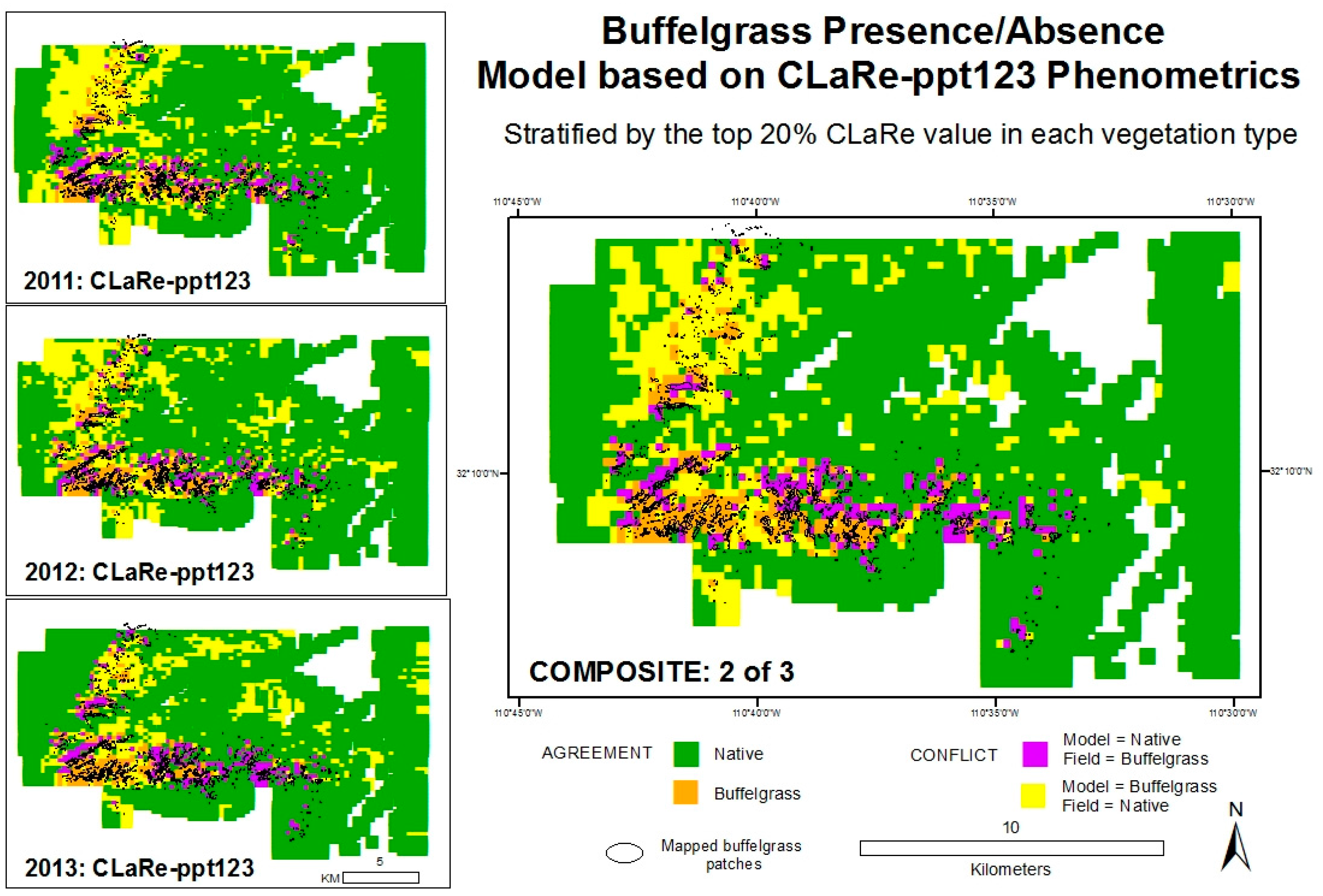
The second set of models was developed to be easily created with no prior knowledge of buffelgrass distribution. Based on exploratory statistics (
Table 2) and modeling results, these models used the CLaRe ppt123 for each year. All CLaRe ppt123 values were extracted for each mapped vegetation type and the top 5th of the highest correlations were mapped as buffelgrass presence (
i.e., the upper 20 percent of calculated correlation values). For modeling and validation purposes, we eliminated the higher elevation vegetation types that are unsuited for buffelgrass (e.g., Madrean pine-oak forest and woodland). The three sub-models show the results for each year (left panels,
Figure 10). The composite model (right image,
Figure 10) maps buffelgrass presence if 2 of 3 sub-models mapped buffelgrass presence. Validation results are shown in the
Appendix Table A2.
Validation results suggest that the three sub-models do a reasonable job identifying known patches of buffelgrass, capturing 45 to 49 percent correctly. The composite models improve the accuracies: composite model 2 of 3 (shown in
Figure 10) has an overall accuracy of 83 percent and correctly maps 46 percent of known buffelgrass. Note the tradeoffs between overall accuracy and the total amount of buffelgrass correctly identified compared to the amount misclassified and missed (
Table A2 in the
Appendix). In all cases, the models show poor user’s accuracies (typically <25%) for mapping buffelgrass, with the model classifying areas as buffelgrass that were confirmed native vegetation in the field. Suggestions for improving the accuracies are presented in the discussion section below.
4.4. Mapping Buffelgrass—When?
Because optimal use of herbicide to control buffelgrass requires that the plant is photosynthetically active when treated, it is important to map not only where buffelgrass is located, but also when it is green. To predict the phenological status of buffelgrass, we analyzed the citizen science data collected at all locations through the Tucson region. The linear equations derived for the correlation analysis relating field observed buffelgrass greenness to various cumulative precipitation totals were solved for precipitation at specified amounts of buffelgrass greenness. We initially solved the equations at each citizen science location, and found a distinct split between sites in the Santa Catalina foothills and sites in the Tucson Mountain area. This is not surprising, given that the geology and soils are very different, with the Tucson Mountains composed dominantly of mafic volcanic rocks and the Santa Catalinas composed of granites and felsic metamorphic schists and gneisses. Furthermore, sites in the Santa Catalinas are typically in foothills with southern aspects whereas sites in the Tucson Mountains are typically on eastern facing slopes; we noted earlier that aspect is likely a factor affecting landscape response to precipitation. In addition, there was a wide range of total observations at each citizen science site, ranging from 4 to 58 (excluding Pima Canyon). We therefore pooled all observations for sites in the Santa Catalina foothills (N = 428) and all sites in the Tucson Mountain area (N = 468).
Results for the Santa Catalina and Tucson Mountain sites (
Table 3 and
Table 4, respectively) show that considerably more rain is required for buffelgrass to achieve equivalent greenness levels in the Santa Catalinas. For example, to achieve the management threshold of greenness for effective herbicide application, results suggest buffelgrass will be 50% green 8 to 16 days after a 24 day period that totals over 46 mm (1.8 inches) and 25 mm (1.0 inches) of rain in the Santa Catalina and Tucson Mountains, respectively. Our research does not answer why this difference exists, though we suggest that soils, slope and geology are factors, but does point out that exact precipitation thresholds will vary by area. In the Tucson region, a conservative threshold based on our results is 46 mm (1.8 inches); buffelgrass in the Tucson Mountains would then be expected to be about 80% green (
Table 3), which still meets the herbicide treatment requirement that it be at least 50% green. In SNP-east, where we were unable to monitor buffelgrass on the ground, similar geology and geomorphology suggests that the thresholds observed in the Santa Catalina sites would be most appropriate to use. Of course, knowledge of these thresholds will evolve and become more accurate as practitioners interact with the landscape. In addition, the following section will show how MODIS data can be used to confirm green up in an area targeted for treatment.
5. Operational Protocol
The research results can be used to create a general protocol for operationally informing management activities related to herbicide treatment of buffelgrass at SNP and the Tucson region. Certain decisions, although produced from the data specific to this area, are likely to be generalizable. For example, the metric CLaRe ppt123 was used to model buffelgrass presence in the landscape for our region. Given the characteristic aggressive response of buffelgrass to precipitation, it is likely this metric will be useful, if not optimal, in other areas as well. Suggested steps for optimizing the timing of herbicide treatment for buffelgrass in the landscape are as follows:
Map where buffelgrass is by using historic MODIS NDVI data and PRISM precipitation data to create CLaRe ppt123 metrics for several years of data. Include any model refinements in this step, as presented in the discussion section. Modeling results from this study suggest that an effective way to screen a region for buffelgrass presence is to extract CLaRe ppt123 metrics (i.e., cumulative precipitation for the three prior eight-day periods) for vulnerable vegetation types, and examine areas with the highest correlation metrics as candidate landscapes for hosting buffelgrass. In our study, good results were achieved by examining the top 5th (highest 20%) of the correlation values. The upper threshold selected can reflect expert knowledge of the extent of buffelgrass invasion in the management area, the size of the area that can be reasonably examined given resource constraints, and the relative vulnerability to invasion of landscapes of concern. Creating composite models from several years of data is shown to improve accuracy; composites are created using CLaRe ppt123 by mapping buffelgrass presence if half or more of the suite of individual annual models map buffelgrass.
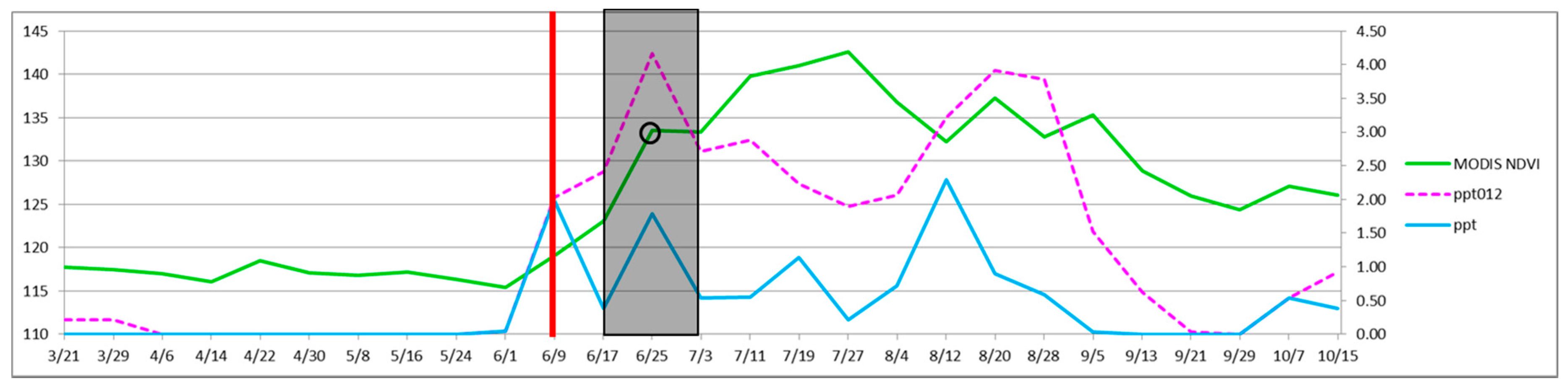
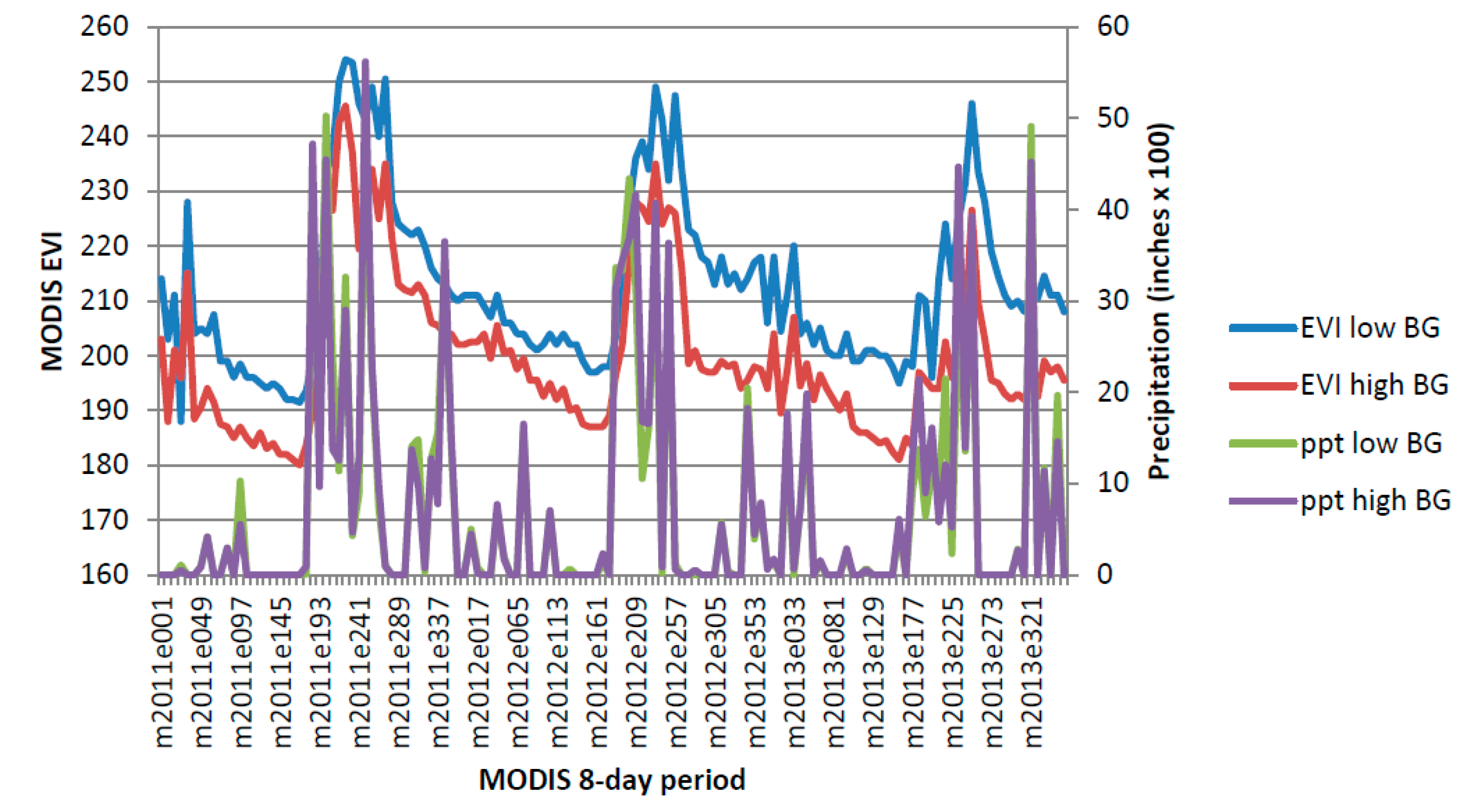
Select areas to target for treatment and collect the MODIS NDVI and PRISM precipitation data at that location. For example, eight-day MODIS (solid green line) and PRISM data (solid blue line) for 2011 at a pixel in SNP-East that contains a patch of high density buffelgrass is shown in
Figure 11. Note that PRISM values are available daily and, as of this writing, eMODIS data, which is the composite NDVI value for the prior seven days, are also available daily. MODIS eight-day composite data used in this study are shown to compare very well with eMODIS data [
44]. This means that it is now possible to access for free PRISM 4-km precipitation data and 250-m eMODIS NDVI data every day that are current through yesterday.
Predict when buffelgrass will be 50 percent green by calculating a running tally of the cumulative precipitation for the past 24 days (dashed magenta line). When the prior 24-day period totals over 46 mm (1.8 inches) of rain (vertical red bar), place crews and aircraft on notice for herbicide application 8 to 16 days from that time (shaded region of graph).
At eight days prior to herbicide application, confirm that the target has greened up using current MODIS data (green line), adjust areas for treatment as needed.
On the day of treatment, confirm that the target has greened up using current MODIS data (open black circle), adjust areas for treatment as needed.
6. Discussion
The two composite models for mapping buffelgrass (
Figure 10 and
Figure 11) are both ~80 percent accurate overall and effective at capturing ~50 percent of known buffelgrass patches, but have poor user’s accuracies (<26 percent). Inspection of the geography of misclassified pixels suggests environmental factors could be affecting the accuracy. In all models, the producer’s error tends to occur in an east-west band near the southern boundary of the park whereas the user’s error tends to occur in the northwest (
Figure 9,
Figure 10 and
Figure 11). This observation suggests that model results may be improved if areas with distinct aspect are isolated before extracting the highest correlations for composite models.
Other factors may contribute to over-mapping buffelgrass patches and poor user’s accuracies: the coarseness of the PRISM precipitation data used (4 km), the accuracy and relevance of the vegetation map, and the presence of other invasive plants, such as Schismus and fountain grass (Cenchrus macrouru) that display similarly aggressive green-up behavior. The model may be improved using finer resolution precipitation data and more accurate maps of vegetation and invasive species. The SWreGAP map was produced using data collected in 2000 through 2002; an update may be beneficial. Although SNP is protected, vegetation changes may have resulted from fire and drought over the 10+ years before the 2012 helicopter mapping survey was conducted.
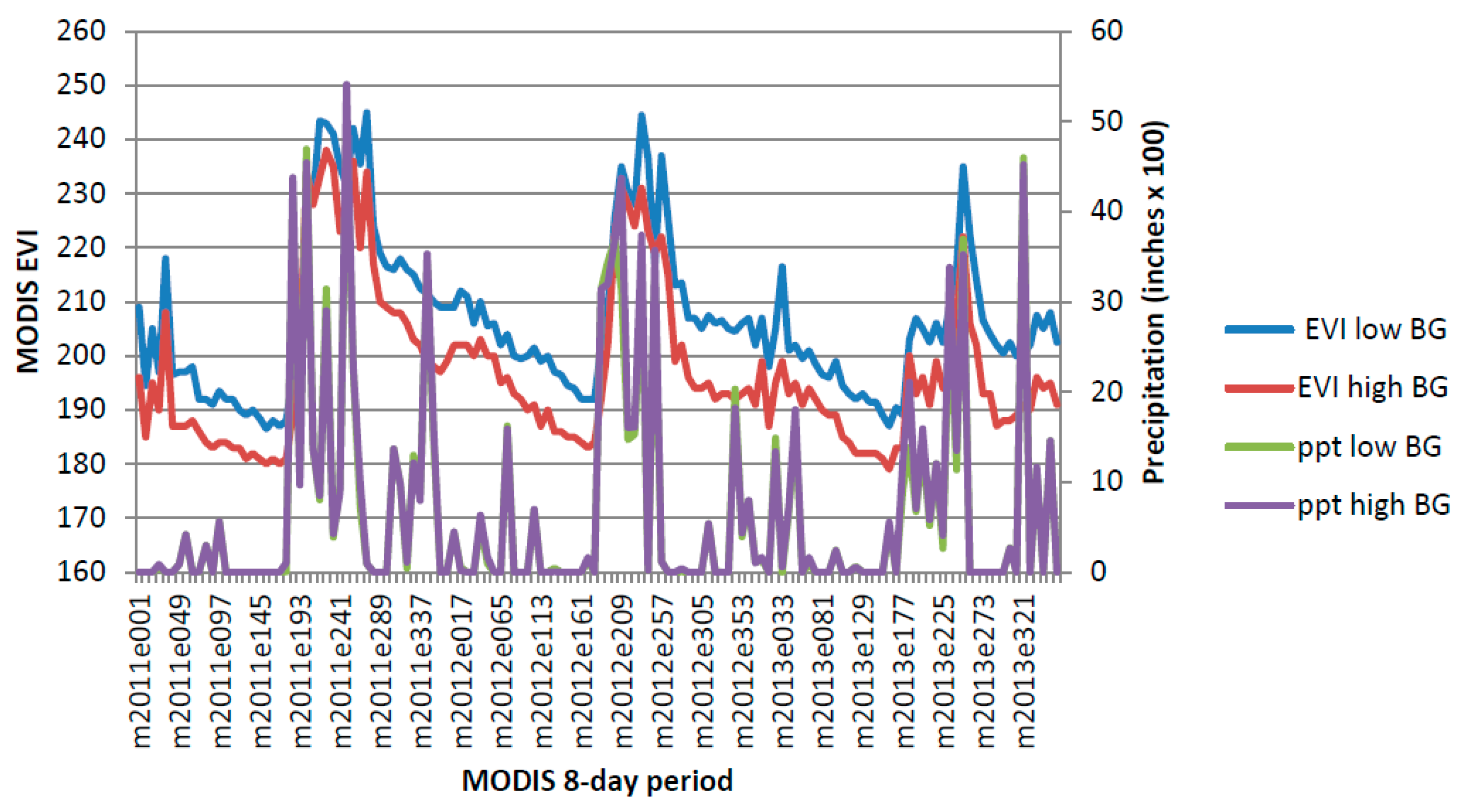
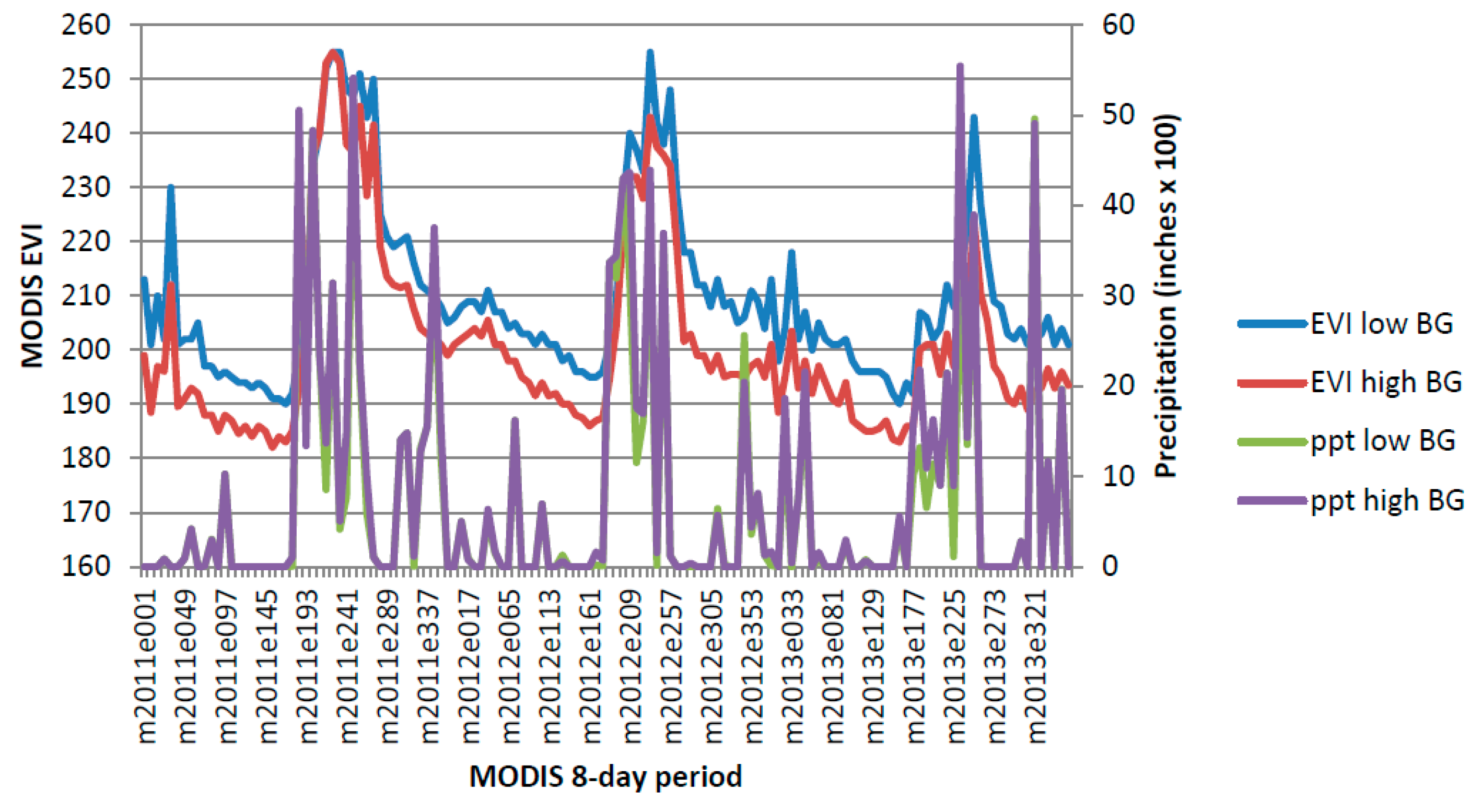
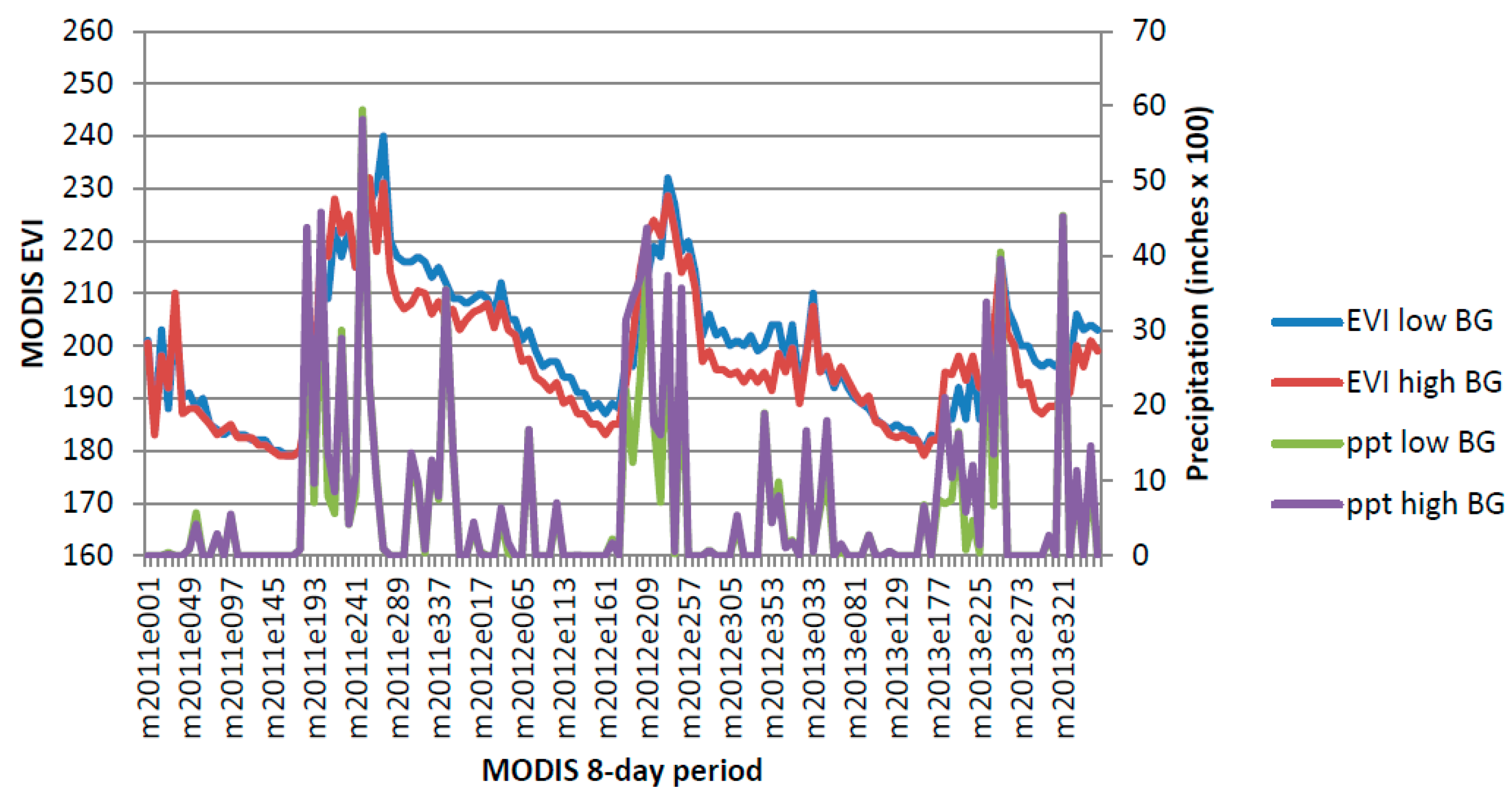
The absolute correlations between MODIS-NDVI and lagged precipitation in the wet year and the dry year were different, with buffelgrass-invaded pixels showing consistently higher values than native vegetation in 2011 (wet), but mixed results in 2013 (dry). Early exploratory statistics revealed that buffelgrass-invaded pixels tend to have overall lower greenness than pixels of native vegetation (
Appendix Figure A1,
Figure A2,
Figure A3 and
Figure A4). This difference likely reflects the ability of buffelgrass to become established in harsher environments, such as drought-stressed south-facing slopes, where there is an overall lower amount of vegetation. This observation may also explain the switch in correlation magnitudes in low precipitation years: The buffelgrass areas are sparser in overall vegetation and remain relatively dormant until sufficient water is applied (thus low correlation in dry years and strong correlation in wet years) whereas most of the native desert vegetation plants maintain some greenness even in dry conditions (thus moderate correlation in both wet and dry years). This finding supports the hypothesis that accuracies will be improved if the study area is stratified by large-scale topographic facets in addition to vegetation type.
Predicting when invasive buffelgrass will be green, calculated using PRISM precipitation data coupled with citizen scientist observation data, revealed a difference between sites collected in the Santa Catalina Mountains and those collected in the Tucson Mountains. Although we hypothesize this difference is mainly due to soils and geology, it is likely that topographic aspect may be a factor, as found in the models mapping buffelgrass distribution. In addition, the predictions for the Santa Catalina Mountains are based on data collected by a few observers over a longer period of time, whereas those in the Tucson Mountains represent a compilation of several observers who collected data over intervals ranging from 4 weeks to 18 months. These predictions can be improved, not only with additional data, but by collecting data within the actual management/study site, as well as by stratifying data using geology, vegetation type and large topographic facets.
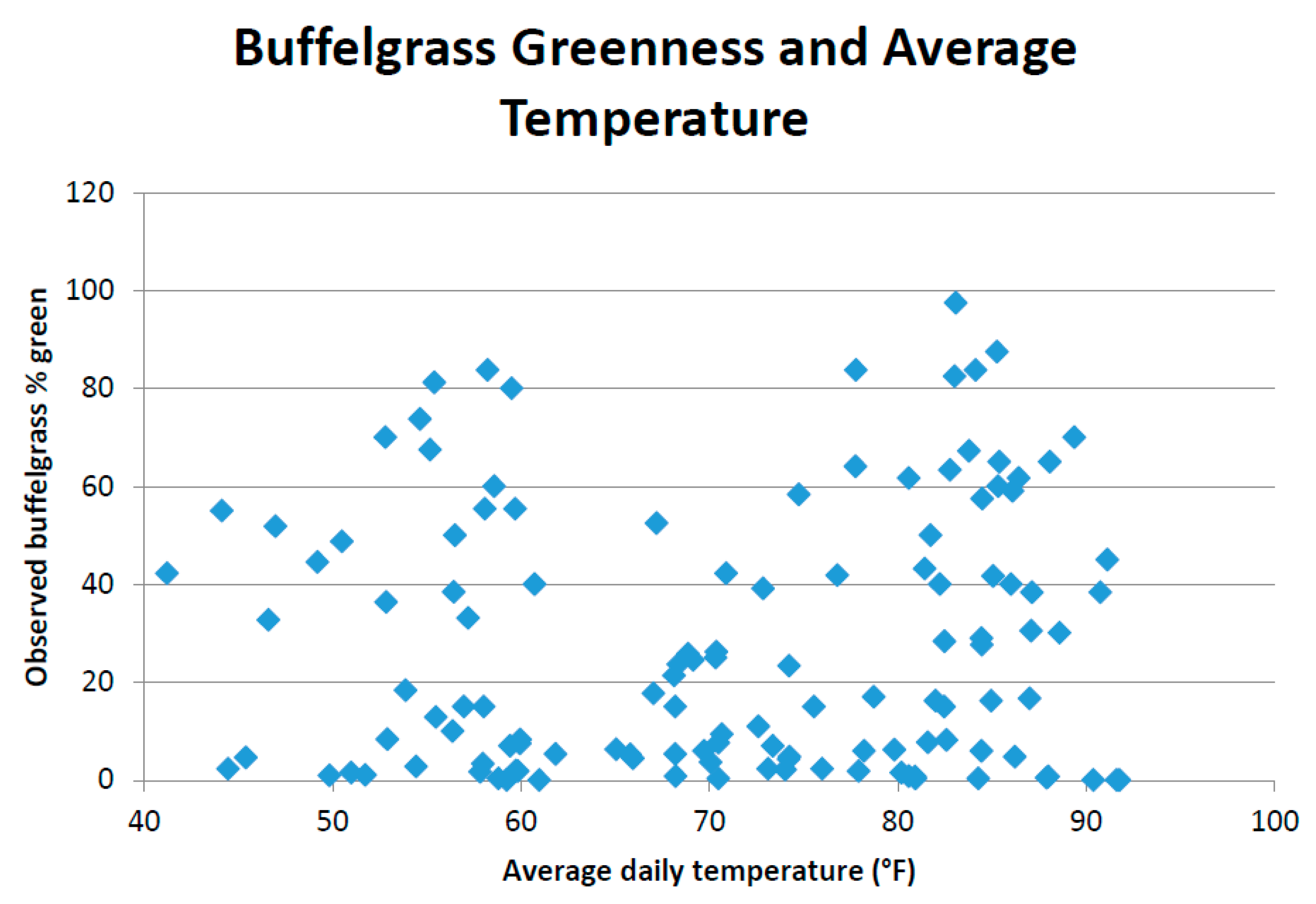
This study pooled annual MODIS NDVI composites and PRISM precipitation data to produce CLaRe metrics. Additional insights will likely be gleaned by not only splitting the data into a winter (cool) season and a summer (warm) season, but also by creating CLaRe metrics using temperature. During exploratory analyses, when observed buffelgrass greenness at the Pima Canyon site was plotted against daily temperature variables, a bimodal distribution was apparent (see
Appendix Figure A5): Buffelgrass greened up in response to rainfall in both cool and warm seasons, unlike native C
4 grasses that respond primarily to warm-season precipitation [
45]. The cool-season greenup of buffelgrass is likely predicated on reaching a certain threshold for temperature; such relationships can be readily explored and mapped spatially using CLaRe phenometrics.
This study demonstrates the usefulness of CLaRe phenometrics in a specific management application related to control of invasive buffelgrass, but they hold promise for many issues related to dryland vegetation. The CLaRe phenometrics used here explicitly incorporate precipitation and capture the strength of the correlation between the satellite greenness data and precipitation data (both lagged and cumulative). These phenometrics are effective in locating populations of invasive buffelgrass since the grass responds more rapidly and strongly to precipitation events than native vegetation. Even small amounts of invasive buffelgrass in the landscape have a strong effect on the values of these phenometrics. Given that many invasive species are successful because they can out-compete native species for limited resources, it is likely the CLaRe phenometrics will prove valuable for mapping other invasive species of regional extent in dryland ecosystems.
7. Conclusions
Buffelgrass is a noxious invasive plant that threatens to degrade the iconic Sonoran Desert ecosystems by out-competing native species and altering fire regimes. Effective treatment of buffelgrass using herbicide requires knowledge of where buffelgrass is located in the landscape and when it is at least 50 percent green. Optimizing herbicide treatment is crucial for many reasons, including cost, efficacy, potential collateral damage to the ecosystem, public opinion, and social concerns. Our research enables the targeted and strategic application of buffelgrass herbicide by using remote sensing data to detect when and where buffelgrass is photosynthetically active and predicting when it will be at least 50 percent green.
CLaRe metrics capture the aggressive response of buffelgrass to recent precipitation: buffelgrass-invaded pixels typically display statistically higher values (i.e., stronger correlations, at ρ < 0.05) than pixels of pure native vegetation for all vegetation types in SNP. Composite models created from CLaRe metrics produced validation results with overall accuracies of ~80 percent and correctly mapped ~50 percent of known buffelgrass patches. Results from the study suggest accuracy can be improved by further stratifying the landscape into large-scale topographic facets of similar aspect. Refinements may also be realized by focusing analyses on specific seasons (winter vs. monsoon) and by creating CLaRe phenometrics with temperature data in addition to precipitation, especially in the winter rainy season.
Citizen science observations at Pima Canyon were key in linking the greenness observed on the ground to the satellite-based MODIS-NDVI data. In addition, the citizen science observations from across the region allowed for the prediction of when buffelgrass will be at least 50 percent green and thus suitable for effective herbicide treatment. Two distinct environments in the Tucson area (Tucson Mountains vs. Santa Catalina Mountains) with different substrates (mafic volcanic vs. alkaline igneous/metamorphic) and aspects (north and east vs. south and west) give two distinct answers. Buffelgrass is predicted to be at least 50 percent green 8 to 16 days after a 24-day period with cumulative rainfall totals of 46 mm (1.8 inches) in the Santa Catalina Mountains and 25 mm (1.0 inches) in the Tucson Mountains.
The phenometrics introduced here are a new and innovative suite of metrics that are proven effective in mapping when and where invasive buffelgrass is green in Saguaro National Park near Tucson, Arizona. The ability to monitor and interpret trends in land surface phenology informs science-based land management. In contrast to temperate regions, which respond to the annual solar cycle, producing predictable greenness curves readily captured by traditional phenometrics, drylands respond to precipitation, which can be erratic. As such, the “start of season” in drylands is more correctly seen to be the onset of a significant precipitation event, such as the monsoon. The CLaRe phenometrics capture the landscape response to climate and will complement the current temperate-zone phenometrics; they will prove broadly useful for many applications, including monitoring dryland ecosystems, mapping invasive species, habitat modeling, and vegetation classification.
Acknowledgments
We wish to thank the National Park Service and Dana Backer, in particular, for supplying us with data and critical feedback on the methods used here. Data were provided by the USA National Phenology Network and the many participants who contribute to its Nature’s Notebook program. The USGS (Land Change Science, Land Remote Sensing and National Park Monitoring Project within the Status & Trends Program) provided funding for this research. Jessica Walker was supported by a USGS Mendenhall Research Fellowship during this work. We appreciate the thoughtful and constructive comments from our three anonymous reviewers and USGS internal reviewer Joel Sankey. Any use of trade, firm, or product names is for descriptive purposes only and does not imply endorsement by the U.S. Government.
Author Contributions
Cynthia S. A. Wallace conceived and designed the study with input from Caroline Patrick-Birdwell and guidance from Jake F. Weltzin; Jake F. Weltzin collected the Pima Canyon dataset; Caroline Patrick-Birdwell, Jake F. Weltzin and Cynthia S. A. Wallace recruited and trained citizen scientist volunteers; Caroline Patrick-Birdwell checked in with and engaged the citizen scientists; Cynthia S. A. Wallace, Jessica J. Walker, Helen Raichle and Susan M. Skirvin performed the data processing; Cynthia S. A. Wallace, Jessica J. Walker and Susan M. Skirvin analyzed the results; Cynthia S. A. Wallace and Jessica J. Walker wrote the paper.
Conflicts of Interest
The authors declare no conflict of interest.
Appendix
Table A1.
Accuracy assessment of models derived from 2011 CLaRe Metrics.
Table A1.
Accuracy assessment of models derived from 2011 CLaRe Metrics.
| 2011 CLaRe Phenometrics Stratified by Average BG Value | 2011 Composite Models |
|---|
| ppt12 | NTV-field | BG-field | Total | User’s | 1 of 3 | NTV-field | BG-field | Total | User’s |
| NTV-mod | 3390 a | 174 b | 3564 | 95.12 | NTV-model | 2960 a | 137 b | 3097 | 95.58 |
| BG-model | 1108 c | 281 d | 1389 | 20.23 | BG-model | 1538 c | 318 d | 1856 | 17.13 |
| Total | 4498 | 455 | 4953 | | Total | 4498 | 455 | 4953 | |
| Producer’s | 75.37 | 61.76 | | 74.12 | Producer’s | 65.81 | 69.89 | | 66.18 |
| ppt123 | NTV-field | BG-field | Total | User’s | 2 of 3 | NTV-field | BG-field | Total | User’s |
| NTV-mod | 3305 a | 182 b | 3487 | 94.78 | NTV-model | 3339 a | 179 b | 3518 | 94.91 |
| BG-model | 1193 c | 273 d | 1466 | 18.62 | BG-model | 1159 c | 276 d | 1435 | 19.23 |
| Total | 4498 | 455 | 4953 | | Total | 4498 | 455 | 4953 | |
| Producer’s | 73.48 | 60.00 | | 72.24 | Producer’s | 74.23 | 60.66 | | 72.99 |
| ppt123 | NTV-field | BG-field | Total | User’s | 3 of 3 | NTV-field | BG-field | Total | User’s |
| NTV-mod | 3186 a | 161 b | 3347 | 95.19 | NTV-model | 3582 a | 201 b | 3783 | 94.69 |
| BG-model | 1312 c | 294 d | 1606 | 18.31 | BG-model | 916 c | 254 d | 1170 | 21.71 |
| Total | 4498 | 455 | 4953 | | Total | 4498 | 455 | 4953 | |
| Producer’s | 70.83 | 64.62 | | 70.26 | Producer’s | 79.64 | 55.82 | | 77.45 |
Table A2.
Accuracy assessment of models derived from the top 20 percent of GCG ppt123 metrics.
Table A2.
Accuracy assessment of models derived from the top 20 percent of GCG ppt123 metrics.
| Top 20 Percent CLaRe-ppt123 in Each Vegetation Type | Top 20 Percent Composite Models |
|---|
| 2011 | NTV-field | BG-field | Total | User’s | 1 of 3 | NTV-field | BG-field | Total | User’s |
| NTV-mod | 3715 a | 250 b | 3965 | 93.69 | NTV-model | 2909 a | 128 b | 3037 | 95.79 |
| BG-model | 783 c | 205 d | 988 | 20.75 | BG-model | 1589 c | 327 d | 1916 | 17.07 |
| Total | 4498 | 455 | 4953 | | Total | 4498 | 455 | 4953 | |
| Producer’s | 82.59 | 45.05 | | 79.14 | Producer’s | 64.67 | 71.87 | | 65.33 |
| 2012 | NTV-field | BG-field | Total | User’s | 2 of 3 | NTV-field | BG-field | Total | User’s |
| NTV-mod | 3731 a | 234 b | 3965 | 94.10 | NTV-model | 3900 a | 246 b | 4146 | 94.07 |
| BG-model | 767 c | 221 d | 988 | 22.37 | BG-model | 598 c | 209 d | 807 | 25.90 |
| Total | 4498 | 455 | 4953 | | Total | 4498 | 455 | 4953 | |
| Producer’s | 82.95 | 48.57 | | 79.79 | Producer’s | 86.71 | 45.93 | | 82.96 |
| 2013 | 4125 | 201 | Total | User’s | 3 of 3 | NTV-field | BG-field | Total | User’s |
| NTV-mod | 3699 a | 264 b | 3963 | 93.34 | NTV-model | 4336 a | 374 b | 4710 | 92.06 |
| BG-model | 799 c | 191 d | 990 | 19.29 | BG-model | 162 c | 81 d | 243 | 33.33 |
| Total | 4498 | 455 | 4953 | | Total | 4498 | 455 | 4953 | |
| Producer’s | 82.24 | 41.98 | | 78.54 | Producer’s | 96.40 | 17.80 | | 89.18 |
Figure A1.
Apacherian-Chihuahuan Piedmont Semi-Desert Grassland and Steppe 2011–2013.
Figure A1.
Apacherian-Chihuahuan Piedmont Semi-Desert Grassland and Steppe 2011–2013.
Figure A2.
Chihuahuan Creosotebush, Mixed Desert and Thorn Scrub 2011–2013.
Figure A2.
Chihuahuan Creosotebush, Mixed Desert and Thorn Scrub 2011–2013.
Figure A3.
Chihuahuan Mixed Salt Desert Scrub 2011–2013.
Figure A3.
Chihuahuan Mixed Salt Desert Scrub 2011–2013.
Figure A4.
Sonoran Paloverde-Mixed Cacti Desert Scrub 2011–2013.
Figure A4.
Sonoran Paloverde-Mixed Cacti Desert Scrub 2011–2013.
Figure A5.
Bimodal distribution of buffelgrass greenness over range of average daily temperature during 8-day MODIS composite period.
Figure A5.
Bimodal distribution of buffelgrass greenness over range of average daily temperature during 8-day MODIS composite period.
References
- Halvorson, W.L.; Guertin, P. USGS Weeds in the West Project: Status of Introduced Plants in Southern Arizona Parks. Available online: http://www.buffelgrass.org/sites/default/files/pennfacts.pdf (accessed on 5 May 2015).
- Pimentel, D.; Zuniga, R.; Morrison, D. Update on the environmental and economic costs associated with alien-invasive species in the United States. Ecol. Econ. 2005, 52, 273–288. [Google Scholar] [CrossRef]
- Westbrooks, R.G. Federal Interagency Coordination for Invasive Plant Issues-The Federal Interagency Committee for the Management of Noxious and Exotic Weeds (FICMNEW); American Chemical Society: Washington, DC, USA, 1998; p. 490. [Google Scholar]
- Wilson, M.F.; Leigh, L.; Felger, R.S. Invasive exotic plants in the Sonoran Desert. In Invasive Exotic Species in the Sonoran Region; Tellman, B., Ed.; The University of Arizona Press: Tucson, AZ, USA, 2002; pp. 81–90. [Google Scholar]
- Nabhan, G.P.; West, P.; Felger, R.S.; O’Brien, M.; O’Brien, J.; Van Devender, T.R.; Guererro, A.L.R.; McLaughlin, S.P.; Jenkins, P.; Stromberg, J.C. Naturalized exotic species in the Sonoran Region. In Invasive Exotic Species in the Sonoran Region; Tellman, B., Ed.; The University of Arizona Press: Tucson, AZ, USA, 2002; pp. 346–355. [Google Scholar]
- Stevens, J.; Falk, D.A. Can buffelgrass invasions be controlled in the American Southwest? Using invasion ecology teory to understand bufelgrass success and develop comprehensive restoration and management. Ecol. Restor. 2009, 27, 417–427. [Google Scholar] [CrossRef]
- Frid, L.; Holcombe, T.; Morisette, J.T.; Olsson, A.D.; Brigham, L.; Bean, T.M.; Betancourt, J.L.; Bryan, K. Using state-and-transition modeling to account for imperfect detection in invasive species management. Invasive Plant Sci. Manag. 2013, 6, 36–47. [Google Scholar] [CrossRef]
- Williams, D.; Baruch, Z. African grass invasion in the Americas: Ecosystem consequences and the role of ecophysiology. Biol. Invasions 2000, 2, 123–140. [Google Scholar] [CrossRef]
- Búrquez-Montijo, A.; Miller, M.E.; Martínez-Yrízar, A. Mexican grasslands, thornscrub, and the transformation of the Sonoran desert by invasive exotic buffelgrass (Pennisetum ciliare). In Invasive Exotic Species in the Sonoran Region; Tellman, B., Ed.; Unversity of Arizona Press: Tucson, AZ, USA, 2002; pp. 126–146. [Google Scholar]
- McDonald, C.J.; McPherson, G.R. Creating hotter fires in the Sonoran Desert: Buffelgrass produces copious fuels and high fire temperatures. Fire Ecol. 2013, 9, 26–39. [Google Scholar] [CrossRef]
- Morales-Romero, D.; Molina-Freaner, F. Influence of buffelgrass pasture conversion on the regeneration and reproduction of the columnar cactus, Pachycereus pecten-aboriginum, in Northwestern Mexico. J. Arid Environ. 2008, 72, 228–237. [Google Scholar] [CrossRef]
- Stevens, J.M.; Fehmi, J.S. Competitive effect of two nonnative grasses on a native grass in southern Arizona. Invasive Plant Sci. Manag. 2009, 2, 379–385. [Google Scholar] [CrossRef]
- Franklin, K.A.; Lyons, K.; Nagler, P.L.; Lampkin, D.; Glenn, E.P.; Molina-Freaner, F.; Markow, T.; Huete, A.R. Buffelgrass (Pennisetum ciliare) land conversion and productivity in the plains of Sonora, Mexico. Biol. Conserv. 2006, 127, 62–71. [Google Scholar] [CrossRef]
- D’Antonio, C.M.; Vitousek, P.M. Biological invasions by exotic grasses, the grass fire cycle, and global change. Annu. Rev. Ecol. Syst. 1992, 23, 63–87. [Google Scholar] [CrossRef]
- Backer, D.; Grissom, P. Buffelgrass Talking Points. Available online: http://www.nps.gov/sagu/learn/nature/upload/BG-Talking-Points-Mar2010.pdf (accessed on 11 October 2015).
- Backer, D.; National Park Service (Saguaro National Park, Tucson, AZ, USA). Personal Communication, 2015.
- National Park Service. Buffelgrass. Available online: http://www.nps.gov/sagu/learn/nature/buffelgrass.htm (accessed on 11 January 2015).
- Restoration Plan: Aerial Treatment of Buffelgrass Complete for 2015. Available online: http://www.nps.gov/sagu/learn/management/restoration-plan.htm (accessed on 12 October 2015).
- Olsson, A.D.; Betancourt, J.; Crimmins, M.A.; Marsh, S.E. Constancy of local spread rates for buffelgrass (Pennisetum ciliare L.) in the Arizona Upland of the Sonoran Desert. J. Arid Environ. 2012, 87, 136–143. [Google Scholar] [CrossRef]
- Cleland, E.E.; Chuine, I.; Menzel, A.; Mooney, H.A.; Schwartz, M.D. Shifting plant phenology in response to global change. Trends Ecol. Evol. 2007, 22, 357–365. [Google Scholar] [CrossRef] [PubMed]
- Bradley, B.A.; Mustard, J.F. Identifying land cover variability distinct from land cover change: Cheatgrass in the Great Basin. Remote Sens. Environ. 2005, 94, 204–213. [Google Scholar] [CrossRef]
- Peterson, E.B. Estimating cover of invasive grass (Bromus) using tobit regression and phenology derived from two dates of Landsat ETM+ data. Int. J. Remote Sens. 2005, 26, 2491–2507. [Google Scholar] [CrossRef]
- Singh, N.; Glenn, N.F. Multitemporal spectral analysis for cheatgrass (Bromus tectorum) classification. Int. J. Remote Sens. 2009, 30, 3441–3462. [Google Scholar] [CrossRef]
- Huang, C.Y.; Geiger, E.L. Climate anomalies provide opportunities for large-scale mapping of non-native plant abundance in desert grasslands. Divers. Distrib. 2008, 14, 875–884. [Google Scholar] [CrossRef]
- Huang, C.; Geiger, E.L.; Van Leeuwen, W.J.D.; Marsh, S.E. Discrimination of invaded and native species sites in a semi-desert grassland using MODIS multi-temporal data. Int. J. Remote Sens. 2009, 30, 897–917. [Google Scholar] [CrossRef]
- Clarke, P.J.; Latz, P.K.; Albrecht, D.E. Long-term changes in semi-arid vegetation: Invasion of an exotic perennial grass has larger effects than rainfall variability. J. Veg. Sci. 2005, 16, 237–248. [Google Scholar] [CrossRef]
- Martin-Rivera, M.H.; Cox, J.R.; Ibarra-Flores, F. Climatic effects on buffelgrass productivity in Sonoran Desert. J. Range Manag. 1995, 48, 60–63. [Google Scholar] [CrossRef]
- Ward, J.P.; Smith, S.E.; McClaran, M.P. Water requirements for emergence of buffelgrass (Pennisetum ciliare). Weed Sci. 2006, 54, 720–725. [Google Scholar] [CrossRef]
- Hanselka, C.W. Buffelgrass: South Texas Wonder Grass. Rangelands 1988, 10, 279–281. [Google Scholar]
- Marshall, V.M.; Lewis, M.M.; Ostendorf, B. Buffel grass (Cenchrus ciliaris) as an invader and threat to biodiversity in arid environments: A review. J. Arid Environ. 2012, 78, 1–12. [Google Scholar] [CrossRef]
- Sheppard, P.; Comrie, A.; Packin, G.D.; Angersbach, K.; Hughes, M. The climate of the US Southwest. Clim. Res. 2002, 21, 219–238. [Google Scholar] [CrossRef]
- Lowry, J.; Ramsey, R.D.; Thomas, K.; Schrupp, D.; Sajwaj, T.; Kirby, J.; Waller, E.; Schrader, S.; Falzarano, S.; Langs, L.; et al. Mapping moderate-scale land-cover over very large geographic areas within a collaborative framework: A case study of the Southwest Regional Gap Analysis Project (SWReGAP). Remote Sens. Environ. 2007, 108, 59–73. [Google Scholar] [CrossRef]
- USGS Global Visualization Viewer. Available online: http://glovis.usgs.gov (accessed on 12 October 2014).
- Vermote, E.F.; Kotchevova, S.Y.; Ray, J.P. MODIS Surface Reflectance User’s Guide. Available online: http://www.modis-sr.ltdri.org/guide/MOD09_UserGuide_v1_3.pdf (accessed on 15 March 2016).
- Denny, E.G.; Gerst, K.L.; Miller-Rushing, A.J.; Tierney, G.L.; Crimmins, T.M.; Enquist, C.A.; Guertin, P.; Rosemartin, A.H.; Schwartz, M.D.; Thomas, K.A.; et al. Standardized phenology monitoring methods to track plant and animal activity for science and resource management applications. Int. J. Biometeorol. 2014, 58, 591–601. [Google Scholar] [CrossRef] [PubMed]
- USA-NPN USA National Phenology Network (2016). Raw Plant and Animal Phenology Data for the United States, 20 August 2010–31 December 2014. Available online: http://www.dx.doi.org/10.5066/F78S4N1V (accessed on 31 March 2015).
- Nature’s Notebook. Available online: https://www.usanpn.org/natures_notebook (accessed on 6 June 2016).
- Tucson Phenology Trail. Available online: https://www.usanpn.org/nn/tucson-phenology-trail (accessed on 6 June 2016).
- USA National Phenology Network (2016). Raw Plant and Animal Phenology Data for the United States, 9 January 2013–31 December 2014. Available online: http://www.dx.doi.org/10.5066/F78S4N1V (accessed on 17 April 2015).
- MesoWest. Available online: http://mesowest.utah.edu/ (accessed on 1 October 2014).
- PRISM Climate Group. Available online: http://www.prism.oregonstate.edu (accessed on 9 September 2014).
- National Weather Service Forecast Office Monsoon Statistics for Tucson (1895–2015). Available online: http://www.wrh.noaa.gov/twc/monsoon/monsoon.php (accessed on 6 June 2016).
- NatureServe Conservation Tools and Services. Available online: http://www.natureserve.org/conservation-tools/terrestrial-ecological-systems-united-states (accessed on 6 June 2016).
- Brown, J.F.; Howard, D.; Wylie, B.; Frieze, A.; Ji, L.; Gacke, C. Application-ready expedited MODIS data for operational land surface monitoring of vegetation condition. Remote Sens. 2015, 7, 16226–16240. [Google Scholar] [CrossRef]
- McClaran, M.P. Desert grasslands and grasses. In The Desert Grassland; McClaran, M.P., van Devender, T.R., Eds.; University of Arizona Press: Tucson, AZ, USA, 1995; pp. 1–30. [Google Scholar]
Figure 1.
Examples of (left) a Sonoran Desert landscape showing the characteristic arrangement of patches of native vegetation separated by bare ground; and (right) a Sonoran Desert landscape that has been invaded by buffelgrass, which fills in the open spaces to form a relatively continuous mat of plant material (Photo credits: Dr. Aaryn Olsson).
Figure 2.
Map showing the locations of the citizen science buffelgrass observation sites in Tucson, Arizona, and the outlined polygons of buffelgrass patches in Saguaro National Park East and West. Buffelgrass density is coded as High (H); Medium (M); Low (L) and Trace (T).
Figure 2.
Map showing the locations of the citizen science buffelgrass observation sites in Tucson, Arizona, and the outlined polygons of buffelgrass patches in Saguaro National Park East and West. Buffelgrass density is coded as High (H); Medium (M); Low (L) and Trace (T).
Figure 3.
Visual explanation of the percent buffelgrass raster creation. The polygon coverage of categorical buffelgrass density (A) supplied by Saguaro National Park personnel was converted to a 5-m raster with midpoint densities assigned to each category (B); The average density of buffelgrass within each 250-m MODIS pixel cell (white grid in (B)) was then calculated (C).
Figure 4.
Comparison of citizen science observations of buffelgrass greenness (Greenness) collected at Pima Canyon from 2010 to 2014 with (top) MODIS-NDVI values and (bottom) PRISM precipitation (mm) summed over 8-day intervals. Bottom axis is YR-MO (year-month), right vertical axes of top graph and bottom graph are rescaled NDVI and mm of precipitation, respectively.
Figure 5.
Graph of correlation coefficients between cumulative precipitation amounts at Pima Canyon field and both observed percent greenness (“Field Obs”) and MODIS NDVI values for 2010–2013. X axis values correspond to the number of 8-day time periods over which precipitation was summed, with 0 = current time period, 1 = the previous time period, 2 = the previous 2 time periods, etc.
Figure 6.
An example of one of the CLaRe phenometrics mapped in SNP-East for 2011, 2012 and 2013. The CLaRe Phenometric displayed is the correlation between MODIS NDVI and ppt123, i.e., the cumulative precipitation for the three prior 8-day time periods. Notice that a high correlation coefficient indicates a greater probability of buffelgrass presence, as evidenced by the spatial coincidence of mapped buffelgrass patches with the higher image values.
Figure 7.
CLaRe phenometrics of selected native vegetation types at SNP-East. The graph (top) shows correlation coefficients of the linear relationship between MODIS NDVI and a suite of cumulative precipitation values in pixels with native vegetation and no reported buffelgrass. Correlation coefficients are plotted on the Y axis, reflecting the strength of the relationship between MODIS NDVI and cumulative precipitation values. The X axis values correspond to the number of 8-day time periods over which precipitation was summed: 0 = current time period, 1 = previous time period, 2 = previous 2 time periods, etc. Line colors correspond to colors of vegetation types in the map at the bottom. The map shows the dominant SWreGAP vegetation types in each MODIS pixel footprint.
Figure 8.
Correlation coefficients for various amounts of buffelgrass in the five dominant vegetation types at SNP that have buffelgrass invasion. In these graphs, the horizontal axis values represent the number of prior time periods over which precipitation is summed, with 0 = current precipitation, 1 = precipitation from the previous time period, 2 = cumulative precipitation from the previous two time periods, and so on. The table in lower right corner of each panel shows the number of pixels within each density class for the vegetation types.
Figure 9.
Modeled buffelgrass presence-absence based on 2011 CLaRe metrics.
Figure 9.
Modeled buffelgrass presence-absence based on 2011 CLaRe metrics.
Figure 10.
Modeled buffelgrass presence-absence based on the top 20 percent of CLaRe ppt123 metrics.
Figure 10.
Modeled buffelgrass presence-absence based on the top 20 percent of CLaRe ppt123 metrics.
Figure 11.
Monitoring precipitation and MODIS NDVI to optimize timing of herbicide treatment (see
Section 5, steps 2 through 5). The horizontal axis shows the month and day in 2011, beginning March 21. The left vertical axis is a rescaled NDVI value and the right vertical axis is inches of precipitation.
Table 1.
Spearman correlation analysis results for a subset of variable pairings from the Pima Canyon site. Each observation is taken during an 8-day interval corresponding to a MODIS composite period. Field Obs = field-observed greenness; MODIS = MODIS NDVI value; ppt = precipitation received during a given 8-day period; pptx = precipitation received during the time period with lag x; ppt12 = cumulative precipitation received in the prior two time periods (i.e., lags 1 and 2); and ppt123 = cumulative precipitation received in the prior three time periods. Highlighted values exceed 0.50.
| | Field Obs | MODIS | ppt | ppt1 | ppt2 | ppt3 | ppt12 | ppt123 |
|---|
| Field Obs | 1 | | 0.24 | 0.44 | | | | |
| MODIS | | 1 | 0.33 | 0.4 | 0.45 | 0.38 | | |
Table 2.
Descriptive statistics values and
t-test significance between native and buffelgrass-invaded pixels for the dominant vegetation types in SNP that have been invaded by buffelgrass. Three CLaRe metrics are evaluated: ppt12, ppt123 and ppt1234.
Native and
bg are the mean correlation values for pixels of native vegetation and buffelgrass-invaded vegetation, respectively. Highlighted values are significant at ρ = 0.05. For each significantly different native: buffelgrass pair, the higher value is bolded. The five vegetation types shown are (from top to bottom): Apacherian-Chihuahuan Mesquite Upland Scrub, Chihuahuan Mixed Salt Desert Scrub, Apacherian-Chihuahuan Piedmont Semi-Desert Grassland and Steppe, Sonoran Paloverde-Mixed Cacti Desert Scrub, and Madrean Encinal. Monsoon stats: [
42].
Table 2.
Descriptive statistics values and t-test significance between native and buffelgrass-invaded pixels for the dominant vegetation types in SNP that have been invaded by buffelgrass. Three CLaRe metrics are evaluated: ppt12, ppt123 and ppt1234. Native and bg are the mean correlation values for pixels of native vegetation and buffelgrass-invaded vegetation, respectively. Highlighted values are significant at ρ = 0.05. For each significantly different native: buffelgrass pair, the higher value is bolded. The five vegetation types shown are (from top to bottom): Apacherian-Chihuahuan Mesquite Upland Scrub, Chihuahuan Mixed Salt Desert Scrub, Apacherian-Chihuahuan Piedmont Semi-Desert Grassland and Steppe, Sonoran Paloverde-Mixed Cacti Desert Scrub, and Madrean Encinal. Monsoon stats: [42].
| CLaRe-ppt12 | 2011 | 2012 | 2013 |
| type | native | bg | native | bg | native | bg |
| Mesquite Scrub | | | 0.430 | 0.426 | 0.347 | 0.351 |
| Salt Desert Scrub | | | | | 0.278 | 0.248 |
| Grassland & Steppe | | | | | | |
| Sonoran Paloverde | | | | | | |
| Madrean Encinal | | | | | | |
| CLaRe-ppt123 | 2011 | 2012 | 2013 |
| type | native | bg | native | bg | native | bg |
| Mesquite Scrub | 0.736 | 0.745 | 0.451 | 0.444 | 0.399 | 0.403 |
| Salt Desert Scrub | | | | | | |
| Grassland & Steppe | | | | | | |
| Sonoran Paloverde | | | 0.366 | 0.460 | 0.439 | 0.446 |
| Madrean Encinal | | | | | | |
| CLaRe-ppt1234 | 2011 | 2012 | 2013 |
| type | native | bg | native | bg | native | bg |
| Mesquite Scrub | 0.787 | 0.782 | 0.520 | 0.506 | 0.482 | 0.481 |
| Salt Desert Scrub | | | | | | |
| Grassland & Steppe | | | | | 0.548 | 0.597 |
| Sonoran Paloverde | | | | | | |
| Madrean Encinal | | | | | | |
Table 3.
Santa Catalinas cumulative rainfall amounts required to produced 50, 70 and 90 percent buffelgrass greenness. Yellow highlights R2 values greater than 0.50.
Table 3.
Santa Catalinas cumulative rainfall amounts required to produced 50, 70 and 90 percent buffelgrass greenness. Yellow highlights R2 values greater than 0.50.
| 50% | Composite | 70% | Composite | 90% | Composite |
|---|
| | ppt (in) | R2 | | ppt (in) | R2 | | ppt (in) | R2 |
|---|
| lag12 | 1.46 | 0.38 | lag12 | 2.38 | 0.38 | lag12 | 3.31 | 0.38 |
| lag123 | 1.80 | | lag123 | 2.77 | | lag123 | 3.75 | |
| lag23 | 1.42 | 0.41 | lag23 | 2.31 | 0.41 | lag23 | 3.19 | 0.41 |
| lag234 | 1.80 | | lag234 | 2.78 | | lag234 | 3.77 | |
Table 4.
Tucson Mountains cumulative rainfall amounts required to produced 50, 70 and 90 percent buffelgrass greenness. Yellow highlights R2 values greater than 0.50.
Table 4.
Tucson Mountains cumulative rainfall amounts required to produced 50, 70 and 90 percent buffelgrass greenness. Yellow highlights R2 values greater than 0.50.
| 50% | Composite | 70% | Composite | 90% | Composite |
|---|
| | ppt (in) | R2 | | ppt (in) | R2 | | ppt (in) | R2 |
|---|
| lag12 | 0.75 | | lag12 | 1.22 | | lag12 | 1.68 | |
| lag123 | 0.99 | | lag123 | 1.54 | | lag123 | 2.09 | |
| lag23 | 0.68 | 0.49 | lag23 | 1.12 | 0.49 | lag23 | 1.56 | 0.49 |
| lag234 | 0.94 | | lag234 | 1.49 | | lag234 | 2.04 | |
© 2016 by the authors; licensee MDPI, Basel, Switzerland. This article is an open access article distributed under the terms and conditions of the Creative Commons Attribution (CC-BY) license (http://creativecommons.org/licenses/by/4.0/).


 ,
, 
