Abstract
Tidal creeks are small estuarine watersheds characterized by low freshwater input, marine to brackish salinity, and subtidal, intertidal, and supratidal habitats. Most people are familiar with large rivers and estuaries, but the smaller tidal watersheds comprise a greater percentage of the coastline. As the population along coasts rises there is growing concern about water quality and increased sedimentation rates. Therefore, these smaller tidal creek watersheds are at risk to pollution, decreased environmental health, and deterioration of protective salt marshes. The purpose of this study was to test methods for high spatial resolution mapping of benthic (submerged) and emergent habitats as well as the derivation of bathymetry using DigitalGlobe’s WorldView-2 imagery. An intensive field effort was conducted to test and assess several image processing techniques. Results concluded that: (1) supervised habitat classification produced the highest map accuracy (95%); (2) sand, water, scrub/shrub, and docks/rubble were mapped the most accurately at greater than 95%; (3) saltmarsh habitats (high and low density cordgrass, Spartina alterniflora, and black needlerush, Juncus roemerianus), mud, and oyster beds were between 80 and 85% accurate; (4) pan-sharpening and atmospheric correction did not improve map accuracy; (5) LiDAR (light detection and ranging) data increased habitat map accuracy; and (6) WorldView-2 imagery was capable of deriving water depth and these data increased the map accuracy of benthic habitats. The project produced habitat maps for benthic and emergent species at high spatial resolution (4 m2) which will be useful for studying the dynamic processes in this tidal environment. The data and methods developed here could be used by state and local government planning agencies to assess potential long-term changes and develop appropriate management strategies.
1. Introduction
Tidal creek ecosystems are ecologically complex habitats that are home to many species of fish and invertebrates at the boundaries between upland and ocean environments. This dynamic and small estuarine ecosystem provides fish nursery habitat, tidal flushing, and salt marsh habitat that forms the transition zone between submerged, emergent, and upland ecosystems. Their aesthetic beauty makes them prime locations for urban development, leading to changes in the natural landscape and significantly altering the ecological functions of these habitats. In contrast to large riverine watersheds, tidal creeks tend to be relatively small (no more than 5 km in total length) and are prevalent along the Atlantic coast of the United States. The ecological importance and growing urbanization of the coastal landscape make accurate habitat representation necessary in the management of tidal creeks [1,2,3]. The primary objective of this research was to assess the effectiveness of WorldView-2 (WV-2) satellite imagery (DigitalGlobe, Westminster, CO, USA) and light detection and ranging (LiDAR) elevation data for deriving water depth and identifying the distribution and classification of tidal creek habitats. The results will be beneficial in the management and preservation of these habitats and their encompassing wildlife. The methodologies developed can also be accurately and easily implemented in other coastal locations.
Due to the ecological significance of salt marshes, accurate habitat mapping has become an increasingly important component in the management and conservation of these ecosystems. Advances in remote sensing technology have enabled high resolution synoptic views of the landscape, as well as complex image processing algorithms for the derivation of specific habitat characteristics. The variety of multispectral imagery and image processing techniques enables accurate analysis and monitoring of these resources and less time consuming than field mapping [4,5]. This project evaluated the usefulness of WV-2 imagery and LiDAR data for the derivation of water depth and the classification of submerged and emergent habitats.
1.1. Tidal Creek Geomorphology
Although much smaller in comparison to other well-known estuarine systems (i.e., the Albemarle-Pamlico Sound), tidal creek watersheds are a unique characteristic of the southeastern Atlantic coast extending from Norfolk, Virginia, to northern Florida. Tidal creek watersheds develop in shallow, low-energy, high sedimentation areas that often drain into larger bodies of water, such as a sound or bay, that ultimately connect to the ocean. Tidal regime, salinity, elevation, and sedimentation are the most important influences on the development, stability, and productivity of these systems [6].
Tidal creeks have a complex spatial distribution of intertidal communities where salinity, elevation, and tidal regime changes over a short distance. In southeastern North Carolina, low to mid-tidal salt marshes are largely dominated by smooth cordgrass (Spartina alterniflora) which is highly productive in high salinity water where the duration of inundation can last several hours. Smooth cordgrass can also thrive in areas of lower salinity if there is no direct competition with other salt marsh species. As elevation in the watershed increases and inundation time is reduced to 1–2 h, smooth cordgrass is shorter and less dense, and at slightly higher elevations the species diversity increases. Black needlerush (Juncus roemerianus) typically develops in narrow patches along the upper reaches of tidal creeks where salinity is reduced due to freshwater inputs from rainfall surface runoff or groundwater seeps. Needlerush can also occur haphazardly within uniform stands of smooth cordgrass on relic oyster beds that have a slightly higher elevation. Other features that are characteristic of the upper reaches are shallow mud flats and fringing scrub/shrub upland vegetation that is inundated only briefly at high tide or for a longer time frame during a larger spring tide. In the lower reaches of tidal creeks, sand bars and mud flats are interspersed with oysters (Crassostrea virginica) in small patches and large reefs. The complexity of tidal creeks, from higher elevation brackish water to lower elevation, high salinity results in relatively high biodiversity over a small distance of less than a few kilometers.
The balance between tidal hydrodynamics and sediment dynamics from terrestrial to estuarine environments is vital to sustaining salt marshes. Coastal tidal inflow and upland runoff are the two main sediment sources into the salt marsh. Sediment deposition causes the formation of sand bars, marsh vegetation, and mudflats. Alternatively, sediment re-suspension moves sediment from these features out to coastal waters and deepens the creek channels. Under pressure from eustatic sea level rise, tidal salt marshes naturally erode along the shorelines, accrete vertically, and move landward [6]. This process is driven by the deposition of sediment carried with the incoming tide and vegetation recruitment to new areas. If water level increases too quickly, plants may not have enough time to establish in new locations and erosion becomes the dominant process. This process can be exacerbated by climate change and resulting accelerating sea-level rise. Documenting submerged and emergent habitat distribution at high spatial resolution can be used to identify tidal creek watershed processes, quantify the changes, and be useful for developing and implementing management alternatives under varying climate change scenarios.
1.2. Remote Sensing of Coastal Environments
Previous studies have tested high spatial resolution imagery for mapping coastal environments. For example, IKONOS satellite imagery was 20% more accurate than LANDSAT or SPOT imagery [7], and IKONOS performed better than QuickBird [8]. WV-2’s four new spectral bands along with the traditional red, green, blue, and near-infrared (NIR) bands, coupled with a higher spatial resolution (2 m multispectral bands and 0.5 m panchromatic band), are predicted to improve the classification of land and aquatic features (Table 1) [9]. Puetz, et al. [10] compared QuickBird and WV-2 for mapping habitats of the littoral zone off the coast of Maui, Hawaii and WV-2 had a 5% increase in overall map accuracy.

Table 1.
WorldView-2 Specifications.
Pre-processing satellite imagery can also affect the overall accuracy of habitat classification. For example, pan-sharpening is an image fusion method in which lower spatial resolution multispectral bands are fused with a higher spatial resolution panchromatic band to build a multispectral higher-resolution image. Though the spectral response of a pan-sharpened image remains unchanged, the increase in textural information can be beneficial in habitat classification and water depth calculation [2]. Another common pre-processing technique is atmospheric correction which eliminates the effects of aerosols and water vapor in the Earth’s atmosphere [11]. Removing atmospheric influences tends to sharpen the image and improves habitat classification. However, this correction can exacerbate the spatial discontinuity by exemplifying spectral outliers and reduces quality of bathymetric modelling [2].
Determining the elevation relative to a tidal datum is critical for the establishment and productivity of intertidal communities and determines the frequency and duration of tidal flooding experienced by these habitats. LiDAR can provide the high resolution digital elevation models (DEMs) needed to accurately map these intertidal areas [12]. The fusion of LiDAR-based DEMs with multispectral imagery has increased land cover classification accuracy by reducing spectral confusion among classes [12,13,14].
Although LiDAR is effective at measuring surface elevation, laser penetration can be limited in shallow waters and salt marsh vegetation [15,16,17]. Hladik et al. [17] integrated hyperspectral imagery to reduce the error of LiDAR-derived DEMs over salt marsh habitats. Though the integration of LiDAR and hyperspectral imagery are well-suited for surveying intertidal salt marshes, such methods are time consuming and cost prohibitive. LiDAR data has also been used in freshwater wetland environments where there is usually a single species of marsh grass [18]. In this study, WV-2 multispectral imagery and publically available LiDAR data were both examined since the study area has several species of emergent salt marsh and benthic/submerged mapping was required. The data and methods tested in this study may provide a more cost and time effective alternative to other techniques as well as provide options for detailed species mapping.
Several studies have successfully calculated water depth for the deep ocean water (greater than 20 m) using high resolution WV-2 satellite imagery [2,19,20]. Madden [21] successfully calculated bathymetry for water depths greater than 2 m using WV-2 imagery, hydrographic surveys, and the Stumpf et al. [5] relative ratio equation. The Stumpf et al. [5] method is one of the most widely used bathymetry calculations which uses very little input beyond the multispectral image. WV-2’s new spectral bands, in particular the coastal blue and yellow band, are designed to improve feature classification and bathymetry calculations [22]. Incorporating the new bands with the Stumpf et al. (2003) [5] method may provide improvement to bathymetric mapping.
1.3. Study Area
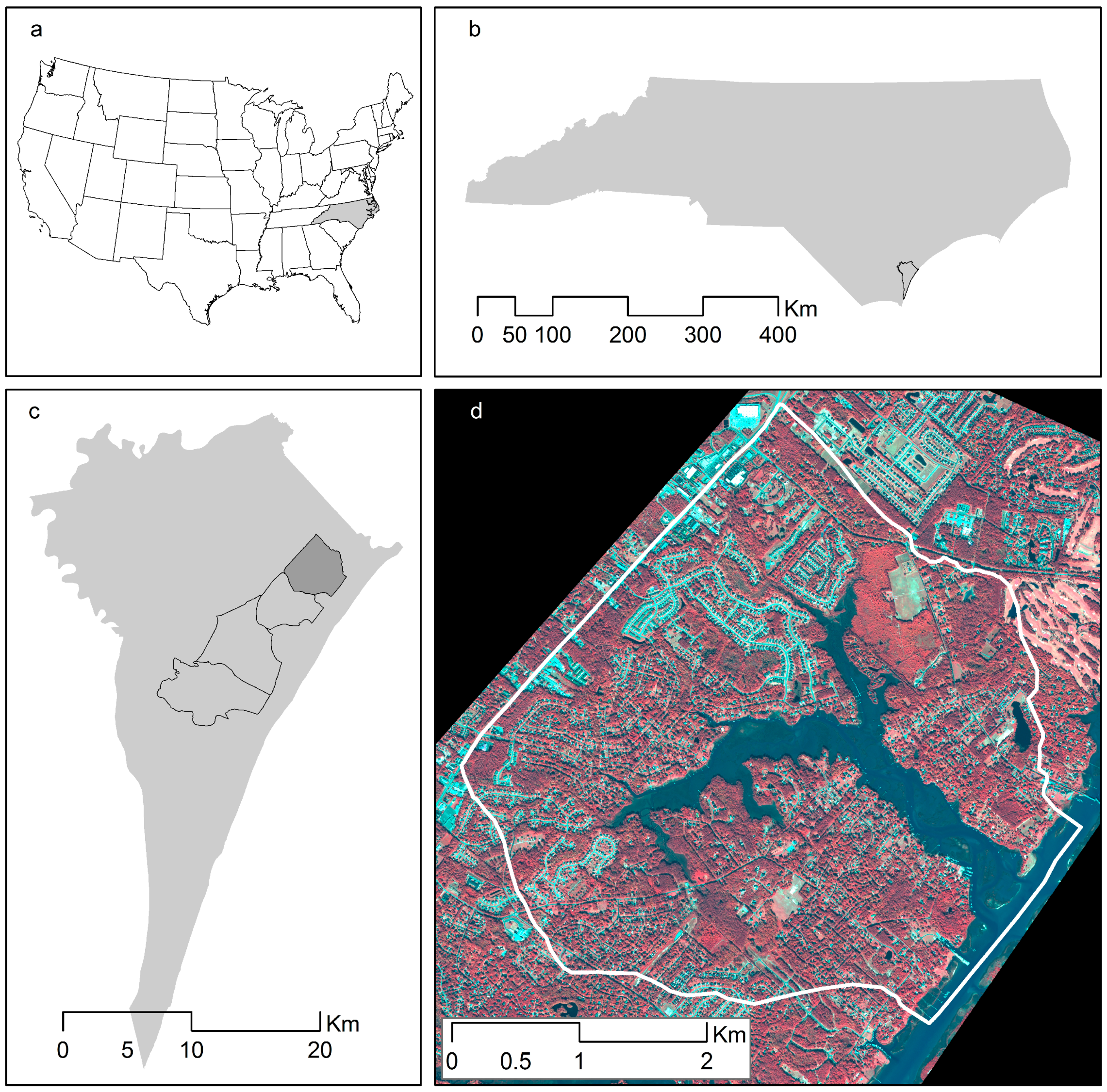
Pages Creek is located in southeastern North Carolina, United States, and drains approximately 4100 acres into the Atlantic Intracoastal Waterway (ICW). Approximately 4500 people live within the boundary of this watershed (Figure 1). The Pages Creek watershed consists mostly of residential neighborhoods and some commercial development. Though some areas of the creek are open to shell fishing (at the lower reaches of the creek), Pages Creek has experienced a decline in the overall water quality. This creek has also seen an increase in bacteria levels during and immediately after rain events, indicating the impacts of storm water runoff from impervious surfaces [23]. As a result, Pages Creek is routinely monitored and regulated through a joint effort between federal and state agencies.
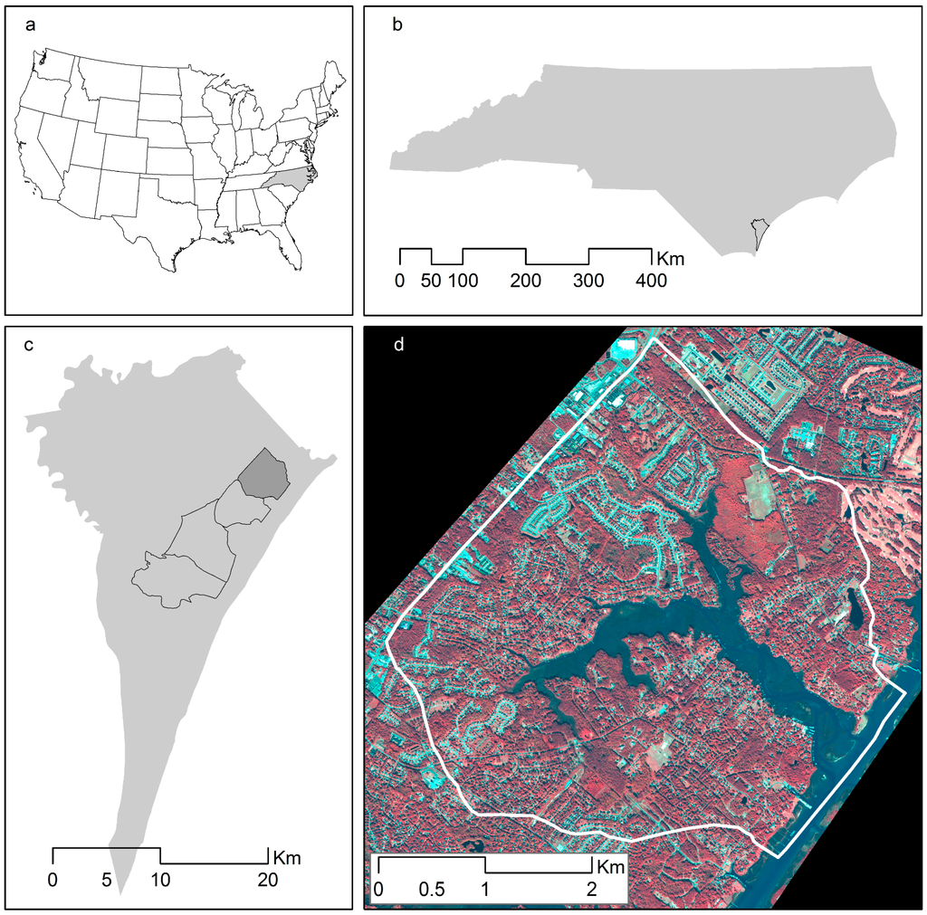
Figure 1.
The study area is located in (a) the Southeastern United States; (b) in the coastal southeast in the state of North Carolina; (c) in New Hanover County; and (d) Pages Creek is one of six tidal creek watersheds in the county.
1.4. Project Significance, Objectives, and Hypotheses
The application of remote sensing analyses to map marsh habitats and shallow water bathymetry has not been done using this combination of fieldwork, WV-2 imagery, and LiDAR data. Similar studies have successfully conducted mapping of marsh habitats using various combinations of imagery and classification methods; however, it has been difficult to distinguish between salt marsh species because of spectral similarities in small geographic areas [2,12,20]. This project takes advantage of the increased spatial resolution and multispectral properties of WV-2 fused with LiDAR to classify habitats and derive bathymetry that has not been possible to this degree of accuracy and precision. The techniques tested in this study will provide a cost-effective and easily repeatable method that may help manage natural resources in these shallow coastal environments.
The following questions were investigated:
- Can WV-2 satellite imagery generate accurate habitat classifications for Pages Creek?
- Does the addition of LiDAR ground elevation data improve habitat classification accuracy?
- What is the best image processing technique for classifying benthic and emergent habitats?
- Can bathymetry be accurately calculated in a shallow tidally influenced location?
2. Methods
To address the research questions, the methods consisted of: (1) gathering and pre-processing WV-2 satellite imagery, LiDAR data and a variety of other existing datasets; (2) conducting a field study to collect ground reference points (GRPs) for submerged and emergent habitats and bathymetry measurements; (3) mapping tidal creek habitats using multiple combinations of imagery, data, and image processing techniques, (4) performing an accuracy assessment to identify the best approaches; and (5) deriving water depth/bathymetry from WorldView-2 imagery (Figure 2).
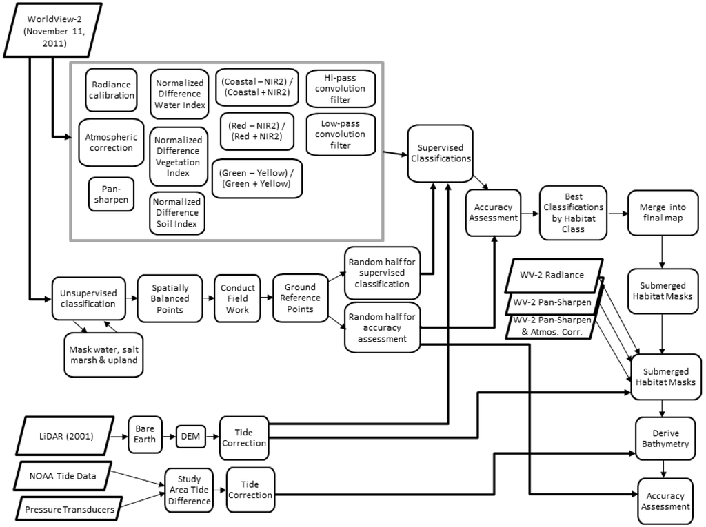
Figure 2.
Project methods consist of multiple image processing techniques to test the accuracy of WorldView-2 for mapping emergent and submerged coastal habitats, extensive fieldwork for training the image processing and accuracy assessment, and incorporating LiDAR data for both image processing and testing the ability of WV-2 to map bathymetry.
2.1. Data and Pre-Processing
2.1.1. WV-2 Satellite Imagery
Launched in 2010, WV-2 is the first commercial polar orbiting high-resolution eight-band multispectral satellite. Operating at an altitude of 770 km in a sun-synchronous orbit, WV-2 has a revisit time of roughly 1.1 days and is capable of collecting up to 1 million km2 [22] of land area per day. WV-2 has 2 m2 spatial resolution in the multispectral bands and 50 cm resolution in the panchromatic band. Along with the standard blue, green, red, and NIR spectral bands; WV-2 has four additional bands, including “coastal” blue, yellow, red edge, and a second NIR band making it the most spectrally diverse commercially available satellite (Table 1).
WV-2 imagery for this project was collected on 11 November 2011 at 16:05 under cloud-free conditions. The imagery was received in tagged image file format (GeoTiFF) with digital numbers stored in 16-bit radiometric resolution. The image radiometry and geometry (UTM projection and WGS84 datum) had been corrected by DigitalGlobe. The multispectral panchromatic bands were received as separate images, providing the opportunity to create a 0.5 m multispectral pan-sharpened image. UNB PanSharp was used for the pan-sharpening of the WV-2 imagery (http://www.fuzego.com/). This is a fairly new algorithm that utilizes a least squares technique to find the best fit between the panchromatic and multispectral pixel values [24]. It was hypothesized that the pan-sharpened image would produce a more accurate habitat map than the original 2 m imagery.
WV-2’s spectral values are received in the form of digital numbers, requiring a two-step process to convert to surface reflectance [25]. First, a specific WorldView radiance calibration function is available in ENVI to convert digital numbers to absolute radiance. The absolute radiance is then transformed to surface reflectance through atmospheric correction. ENVI’s fast line-of-sight atmospheric analysis of spectral hypercubes (FLAASH) tool was used for transforming the WV-2 imagery. Image metadata and regional characteristics of the image scene were used as parameters for FLAASH to fine-tune the atmospheric corrections.
For each WV-2 image (original, pan-sharpened, and pan-sharpened/atmospherically corrected), three indices, three band ratios, and two convolution filters were calculated. Band ratios can be useful for identifying features that single bands may not identify. On a scale of 0 to 1, the ratios classify areas with “in-between” response values, such as vegetation health or moisture content. The band ratios used in this study were those suggested by Wolf (2010) [26]. Convolution filters generate a new value (from −1 to 1) for each pixel by taking the weighted average of the adjacent brightness values. The high-pass filter enhances edges by removing the low frequency and retaining the high frequency components of an image and low-pass filters preserve the low frequency components that tend to smooth the edges. It was hypothesized that the two filters may be able to identify the boundaries or identify the textural differences between the habitat classes. The convolution filters were applied to the NIR2 band using a 3 × 3 kernel size on the original image and a 5 × 5 kernel size for the pan-sharpened and pan-sharpened/atmospherically corrected images.
2.1.2. Light Detection and Ranging (LiDAR) Data
LiDAR is an airborne laser altimeter utilizing a laser scanning device that release a series of light pulses to measure the distance from the sensor to the ground [27]. Each laser pulse can have multiple returns, partially penetrating reef tops, canopy cover, or reaching the ground surface. The ground returns (bare earth points) are used to generate digital elevation models (DEMs). With a high vertical resolution of 20 cm (or less) and spatial resolution of 1 m, coupled with its ability to map large areas in a short amount of time, LiDAR has proven to be advantageous in mapping coastal habitats [2,12,28].
LiDAR data was obtained from the North Carolina Flood Mapping Program (NCFMP) (http://www.ncfloodmaps.com/). NCFMP uses LiDAR data to generate DEMs in order to delineate floodplain boundaries and analyze flood hazards. The LiDAR data was collected using an aerial survey in the spring of 2001, processed (using TerraModel, Trimble Navigation Limited, Sunnyvale, CA, USA) and finalized by 2004 and made available to the public in 2009. The data were downloaded from NCFMP in ASCII points file format representing latitude, longitude, and elevation or depth. Elevation is expressed in 0.001 feet above mean sea level (for more information please refer to http://www.ncfloodmaps.com/). The points were extracted for the Pages Creek study area and, unfortunately, only bare earth points were available. The dataset was horizontally referenced to the North American Datum of 1983 (NAD83) and vertically referenced to North American Vertical Datum of 1988 (NAVD88) with elevation expressed with respect to mean sea level (MSL). The data were converted to mean lower low water (MLLW) using NOAA’s vertical transform tool, VDatum, in order to compare with the NOAA tide gauge at Johnny Mercer’s Pier, Wrightsville Beach. LiDAR elevation data was hypothesized to increase habitat map accuracy.
2.1.3. Other GIS Layers
A variety of public data, such as exiting land cover maps and aerial photography, were gathered from NOAA, USGS, North Carolina Division of Coastal Management, North Carolina One Map, and New Hanover County GIS. All data were compiled into a database and projected to the UTM coordinate system to match the field work and WorldView-2 imagery. The data layers were used to define the watershed and creek area and to do a preliminary investigation of the habitats within the study area. A mask was created to define the study area applied to the original, pan-sharpened, and pan-sharpened/atmospherically-corrected WV-2 images and LiDAR data.
2.2. Field Work
2.2.1. Unsupervised Classification
An unsupervised classification was performed on the WV-2 imagery to identify preliminary habitat classes for planning and conducting field work to collect ground reference points. This method generates a user-specified number of classes based on clustering spectral signatures and then the user groups the classes into meaningful habitat types. ENVI’s K-Mean unsupervised classification tool (Exelis Visual Information Solutions, Inc., Harris Corporation, Melbourne, FL, USA) was performed on the 2 m, multispectral WV-2 image with 20 spectral classes, 25 iterations, and a 5% change threshold. The output image was visually compared with the WV-2 image and the other GIS data layers to create three masks (water, salt marsh, and upland) and the unsupervised classification was repeated on these masked areas and then mosaicked into a map with these classes:
- High Density cordgrass
- Low Density cordgrass
- Black needlerush
- Submerged Oysters
- Emergent Oysters
- Deep Water
- Shallow Water
- Scrub/Shrub
- Docks/Rubble
- Shadows
2.2.2. Spatially-Balanced Points
A spatially balanced sample pattern was used to identify GRPs. Spatially balanced sampling derives points by maximizing the spatial independence within the sample locations [29]. Using the spatially balanced sampling tool, in ArcGIS (Esri, Redlands, CA, USA), and the unsupervised classified map as the input, 30 sample sites were generated for each type of habitat.
Field work was conducted to collect GRPs to be used in the supervised classifications, calculate bathymetry and accuracy assessments. A real-time kinematic (RTK) GPS unit (Trimble 5800 receiver with horizontal accuracy of 10 mm, and vertical accuracies of 20 mm) (Trimble Navigation Limited, Sunnyvale, CA, USA) was used to record the observations at each site. The RTK was pre-programmed with the sample site coordinates and used to navigate to each location. Field work was conducted at Pages Creek over the spring and summer months in 2014, using a small boat and kayaks. The majority of the sites were surveyed by kayak due to shallow water depths at many locations. A two-person team surveyed each site, recording habitat type, GPS location, and a photograph for future reference. During field work, it was determined that mud and sand should also be sampled. Additional sites were surveyed such as transects over deep water channels and perimeters around habitat boundaries.
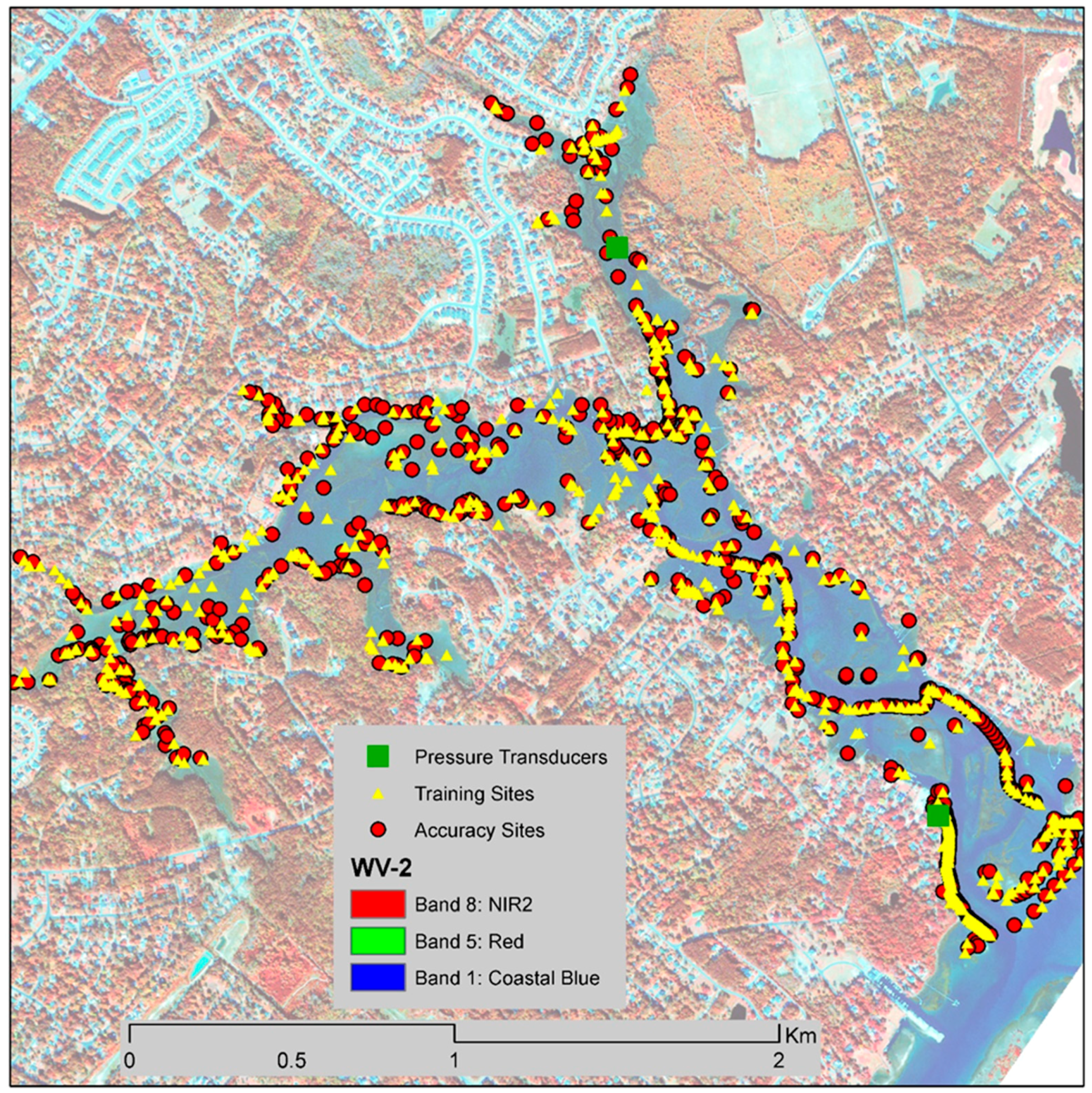
To measure bathymetry, water depths were measured in the field at the same tide height as when the imagery was obtained. At shallow depths, measurements were taken with a meter stick every 10 feet along a 100 m transect made of rope that was secured to PVC pipes. In the deeper water, depths were measured by boat using a Lowrance HDS-7 depth finder (Navico, Inc., San Diego, CA, USA) at 10-second intervals. In total, 25 days of field work, resulting in over 4500 GRPs, were collected (Figure 3).
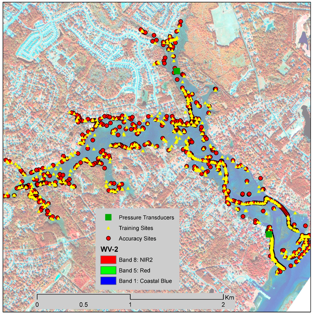
Figure 3.
Location of pressure transducer gauges and ground reference points (GRPs). Half of the GRPs were used for image classification (training sites) and the other half were for classification accuracy assessment.
2.2.3. Tide Correction
The closest NOAA tide gauge to the study site is located approximately at Wrightsville Beach, in the Atlantic Ocean, approximately 11 km from the study area. Due to the substantial distance and shape of the shoreline, there is a difference between the creek tide heights and tide reported at Wrightsville Beach. Therefore, two pressure transducers were deployed to measure the time differences between the NOAA gauge and study area. Tide measurements, using two Levelogger Edge pressure transducers (Solinst, Georgetown, ON, Canada), were collected at the mouth of Pages Creek and upstream over a three-day period. The average rate of change and time difference was a 2 h and 5-min delay from the NOAA gauge to the two locations in Pages Creek. The time data were then interpolated from historical NOAA tide charts for the time of the WV-2 image acquisition which resulted in 3.76 feet (1.146 m) above MLLW. For a detailed explanation of the methods for datum conversion and tide correction, please see Appendix A.
2.3. Habitat Classification
The maximum likelihood supervised image classification technique has been useful in mapping estuarine habitats [17,30]. The maximum likelihood classifier assumes that spectral values within each band, for each class, are normally distributed and calculates the likeliness of a given pixel belonging to a specific class based on the variance and covariance between training class spectra [17]. The GRPs were randomly divided to create a set of training points to be used in the supervised classification and a set of validation points to be used in the accuracy assessment. Given the lag time between the field work and image acquisition, there were a few (less than 10) GRPs that were removed because they were not located within the identified habitat type. Rather than change the classification of the habitat type, it was decided that it is better to remove a GRP that was wrong rather than manually change the designated habitat type. Considering the wealth of GRPs, this was the most appropriate approach. It is better to use good GRPs to train the image classification than include suspicious or potentially wrong GRP data [31,32].
Prior to image classification, spectral plots were computed and it was determined that ten habitat classes were optimal: high-density cordgrass, low-density cordgrass, black needlerush, oysters, sand, mud, deep water, scrub/shrub, docks/rubble, and shadows. To identify band combinations with no spectral overlap correlation matrices resulted in the following band combinations that were tested during image classification:
- Coastal blue, green, red, NIR1
- Blue, yellow, red, NIR2
- Blue, green, red, NIR1
- Coastal Blue, yellow, red edge, NIR2
Classification maps were generated for the original WV-2 image using several combinations of bands, indices, LiDAR generated elevation, and high or low convolution filters. In total, more than 60 classifications were computed and each classified image was then compared to the accuracy assessment points. One of the most common methods for determining the best image classification results is to create a confusion matrix where validation points are compared with the classified map [33]. The confusion matrix summarizes the number and percentage of pixels correctly and incorrectly classified for each class, the errors of omission and commission, overall accuracy, and the kappa coefficient. These statistics are useful when determining how well each class was classified, whereas overall accuracy refers to the percent of all pixels correctly classified for the image. Confusion matrices were generated for each of the classified images using the georeferenced validation points.
2.4. Deriving Bathymetry
Given the spectral variety of the WV-2 imagery and variety of benthic habitats, it was determined that a single equation to predict water depth across the study area was not sufficient. Therefore, to most accurately calculate the bathymetry, masks were created to subset the WV-2 imagery by submerged habitat types: water, oysters, sand, mud, and low-density salt marsh. These five images were then processed to calculate bathymetry equations. The LiDAR data was tested for usefulness to measure water depth. These data are limited because they were collected for terrestrial mapping, not submerged habitats, so first the LiDAR data that was located within the submerged habitats was selected and then these data were randomly divided into two groups: a set for calculating the relative bathymetry and a set for validating the accuracy of the derived bathymetry. Brightness values for each band for all three WV-2 images (radiance, pan-sharpened, and pan-sharpened/atmospherically correct) were extracted from the water depth GRP locations. The data from each band were imported into spreadsheets in order to compare and implement the calculation of water depth.
The first step in the Stumpf et al. [5] method is to calculate the relative bathymetry using the natural log transform of the reflectance values (Equation (1)). This creates a band ratio with the shorter wavelength as the numerator and the longer wavelength as the denominator. The constant n is a fixed value to ensure the values remain positive. Linear regression equations were tested for several band ratio combinations. The relative ratios were plotted against measured GRP depths and the equations from the best fit regression were used to derive absolute bathymetry. Absolute bathymetry was calculated for each submerged habitat type (water, oysters, sand, mud, and low-density marsh). The derived bathymetry was compared with the GRPs that were not used in calibrating the algorithm in order to test the accuracy of the equations.
where, Z = depth, m1 = constant to scale the ratio to depth, n = constant to ensure ratio remains positive, and m0 = offset for a depth of 0 m.
3. Results
3.1. Habitat Classification
The supervised classifications had overall accuracies that ranged from the worst at 83% to the best at 93%, while the overall accuracy of the unsupervised classification was 77.18%. The low-pass convolution filter did not improve any of the image classification results, but the high-pass convolution produced good results. The best overall accuracy was 93.35% and used the band combinations: blue, yellow, red edge, NIR2, NDSI, high-pass convolution, and LiDAR elevation. While the overall accuracy was the best, other band combinations had higher individual habitat class accuracies. Of the more than 60 classification results, nine maps produced the best results (Table 2). The nine combinations were then used in classifying the pan-sharpened and pan-sharpened/atmospherically-corrected images.
Table 2.
Band combinations used for the habitat classification.
All of the best nine classification combinations had high accuracies (all kappa coefficients were greater than 0.81); however, the original WV-2 image produced the most accurate classification with an overall accuracy of 93.35% (kappa = 0.9016). Both the original and pan-sharpened/atmospherically-corrected images outperformed the pan-sharpened image in eight out of nine (89%) maps. The original image outperformed the pan-sharpened/atmospherically-corrected image in five out of nine (56%) corresponding maps. The pan-sharpened image outperformed both the original and pan-sharpened/atmospherically corrected images using the band combination of coastal blue, green, red, NIR-1, NDWI, and LiDAR elevation with an overall accuracy of 92.04% (Table 2).
3.1.1. Habitat Class Accuracy
The accuracy to map individual habitat classes varied between the three images. Pan-sharpened and pan-sharpened/atmospherically-corrected maps had the highest accuracies for high-density cordgrass (producer and user accuracies of 86.84% and 88%, respectively) and sand (producer 100% and user 88.1%), using the band combination of the four new WV-2 bands paired with NDWI, high-pass convolution, and LiDAR. The original WV-2 image did a significantly better job classifying low-density cordgrass, oysters, needlerush, and mud. Scrub/shrub, water, docks/rubble, and shadows were all classified with high accuracies (greater than 88%) in all three maps (Figure 4). In all 60-plus combinations of image classification techniques, there was difficulty classifying the areas covered by shadows. Therefore, a “shadows” class was added and field tested for accuracy. The class comprises less than 5% of the study area and does not affect the overall mapping results.
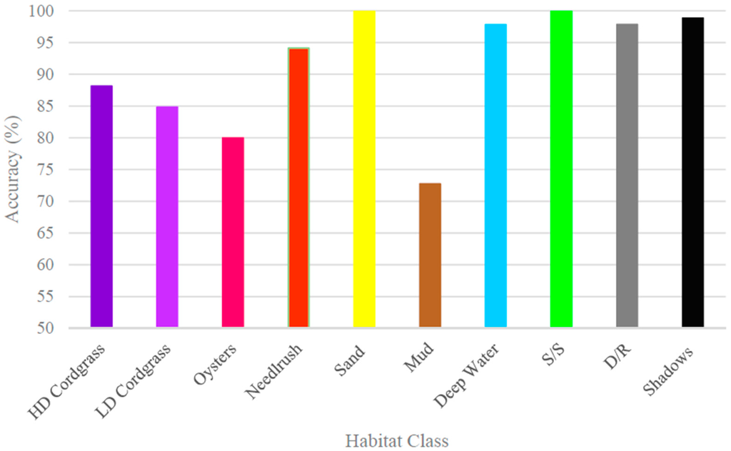
Figure 4.
Map accuracy for each habitat class. Color corresponds with the habitat map in Figure 5.
3.1.2. Fusion of Classified Images
A composite image was created in order to produce a final map that contains the most accurately mapped habitats for the three WV-2 images (original, pan-sharpened, and pan-sharpened/atmospherically-corrected). Each classified grid was imported into ArcMap, converted to polygons with attributes for the producer’s and user’s accuracies from the nine best classification maps. This allowed for the consideration of both the producer’s and user’s accuracy when assigning each grid cell to a class. For example, the same grid cell had different habitat types in some of the classifications and so a series of queries were used to determine the greatest probability for the class for each cell. Once all cells were classified, the final map was assessed for accuracy.
The final merged classifications generated higher overall accuracies, for all three WV-2 images, compared to the original 9 best classifications (Table 3). The original WV-2 image generated the highest overall accuracies at 94.66% (kappa = 0.9203), followed by the pan-sharpened/ atmospherically-corrected image (93.82%), and the pan-sharpened image (92.99%). The original WV-2 outperformed the other images for low-density cordgrass (84.85%) and oysters (80%). Pan-sharpened/atmospherically-corrected images had higher classification accuracy for high-density cordgrass (88.1%) and mud (72.7%). Both the original and pan-sharpened/atmospherically-corrected images were the best for classifying needlerush (76.47%). The most confusion was distinguishing between high- and low-density cordgrass, needlerush, and both cordgrass classes, and oyster and mud. The fused classification method increased the map accuracy for all habitat types. For example, sand, water, scrub/shrub, docks/rubble, and shadows all increased to greater than 94%. The final habitat maps illustrate the habitat in the upper reaches, from the dense salt marsh to the wide mouth of the creek (Figure 5 and Figure 6).
Table 3.
Overall map accuracies for WV-2 supervised classification *.
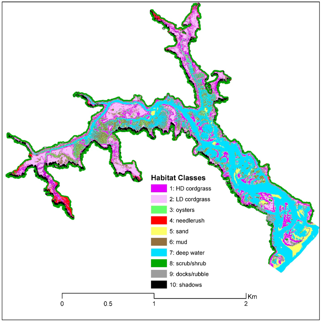
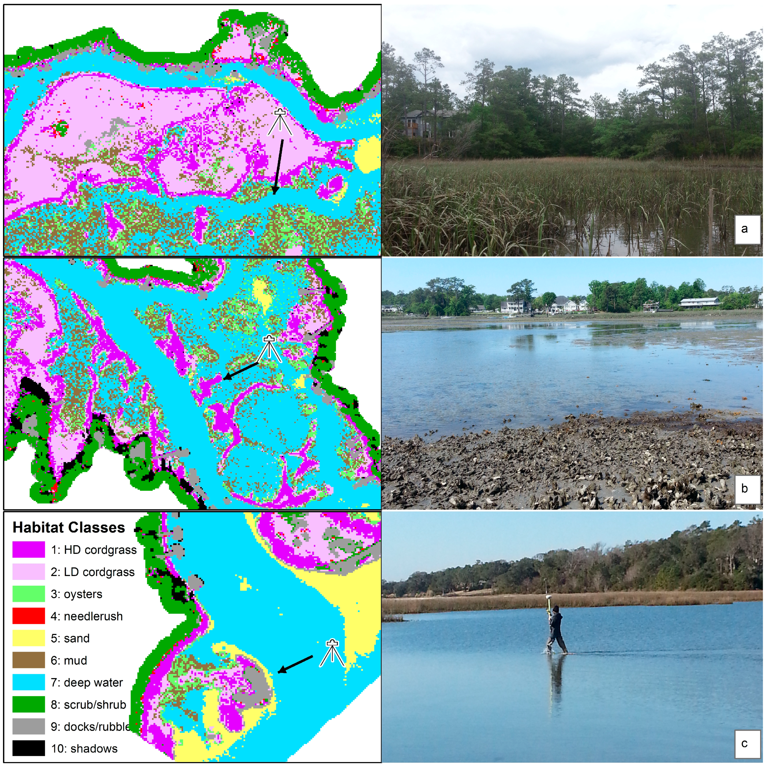
Figure 5.
Final habitat classification for the WV-2 image.

Figure 6.
Example locations in the study area: (a) upper reach with low-density cordgrass in the foreground and high-density cordgrass in the background; (b) middle reach with mud and oysters in the foreground; and (c) estuary mouth of the creek. Camera location and direction are included in each map.
3.2. Derived Bathymetry
Habitat classes (deep water, sand, low density cordgrass, oysters, and mud) from the final habitat map were used to create masks for calculating water depth. Each mask was applied to the LiDAR points which were tested in shallow water areas near the shoreline (depths less than two feet) and GRPs were used for the entire study area including deeper water. Half of the points were used for calibrating the relative bathymetry and the other half were for testing the accuracy. As described in the methods section, the first step to deriving bathymetry is to explore the relationship between band ratios and measured depth at the GRPs. After comparing several band pairs from the three WV-2 images, the pan-sharpened green/yellow ratio had the highest correlation with a R2 value of 0.68.
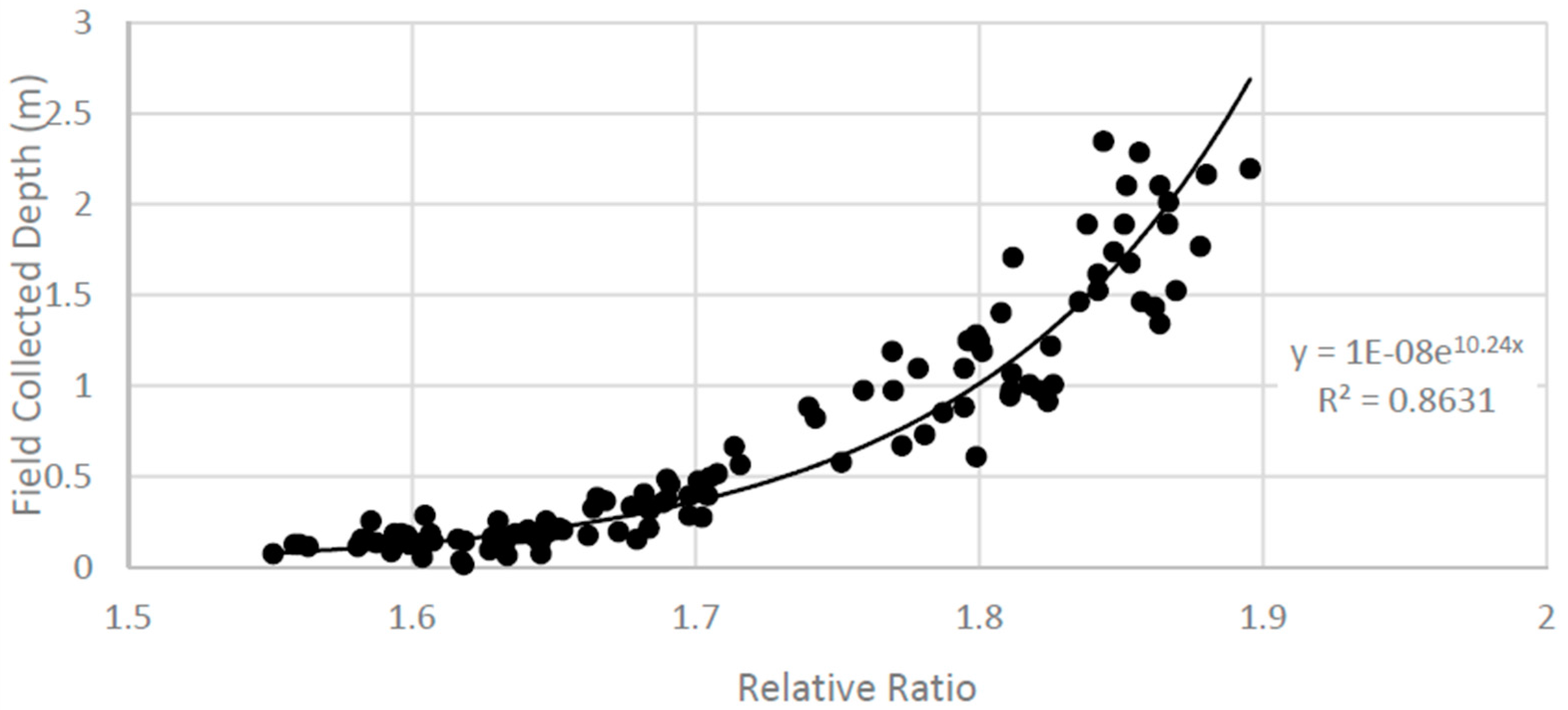
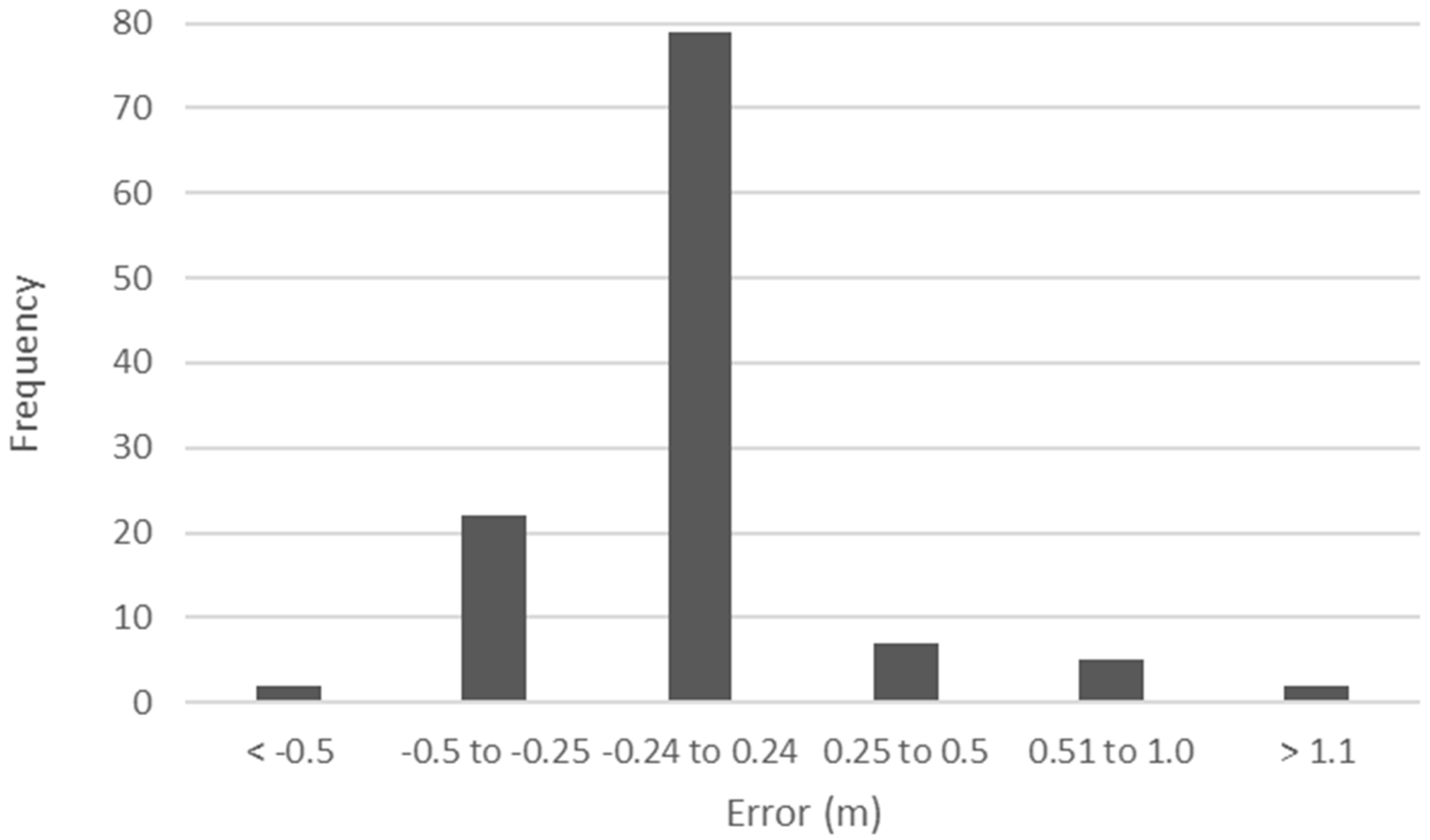
To derive relative bathymetry, the natural log transform was calculated for the green/yellow ratio plotted against the GRPs/LiDAR water depth. Unfortunately, there was no relationship between water depth and reflectance values for areas mapped as mud, low density cordgrass and oysters, so these shallow areas were not used to derive bathymetry. Areas mapped as sand had a linear relationship with an R2 value of 0.75, and deep water had an exponential decay relationship and an R2 value of 0.60. Next, the Stumpf et al. [5] equation was applied to the sand and deep water equations and the predicted depths were compared with the GRP values. The accuracy was lower than expected (R2 of 0.32 and 0.22 for sand and water, respectively) and unacceptable. So, the sand and deep water areas were merged and the regression analysis resulted in a stronger relationship (R2 = 0.86) (Figure 7). Calculated depths were compared to the validation points and show a strong correlation between the calculated depth and field collected depths (R2 = 0.80) (Figure 8). The scatter plot indicates that there is more error predicting deeper water and therefore a comparison was made between the field data and the calculated water depth (Figure 9). A majority (68%) of the sampling sites had less than 0.25 m error which indicates that the model not only had a high R2 result but that the error is acceptable. Interestingly, negative error (where the calculated depth was larger than the actual depth) had a higher frequency than positive error (calculated depth was less than actual). The equation was then used to produce a bathymetric map of the study area (Figure 10).
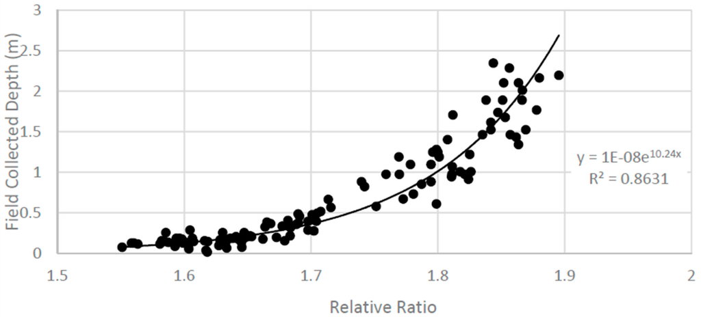
Figure 7.
Relative bathymetry ratio (x-axis) versus measured depth (y-axis). This equation was used to calculate bathymetry for all of the sand and water areas.
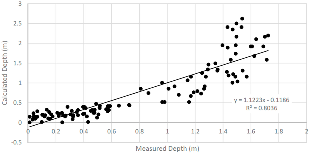
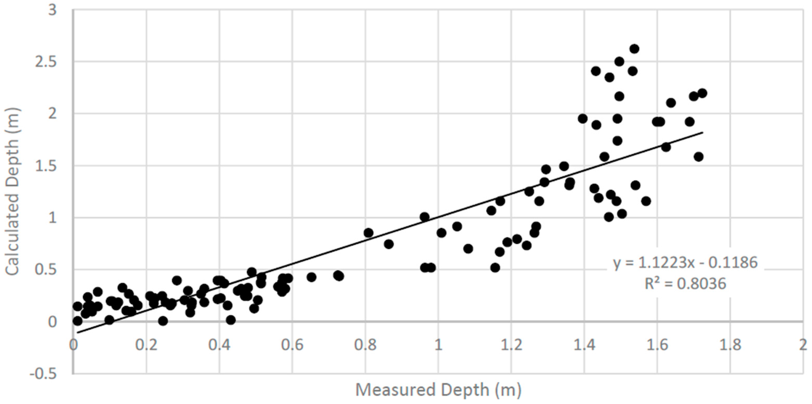
Figure 8.
Measured versus calculated water depth (R2 = 0.80).

Figure 9.
Frequency of error between measured and calculated water depth.
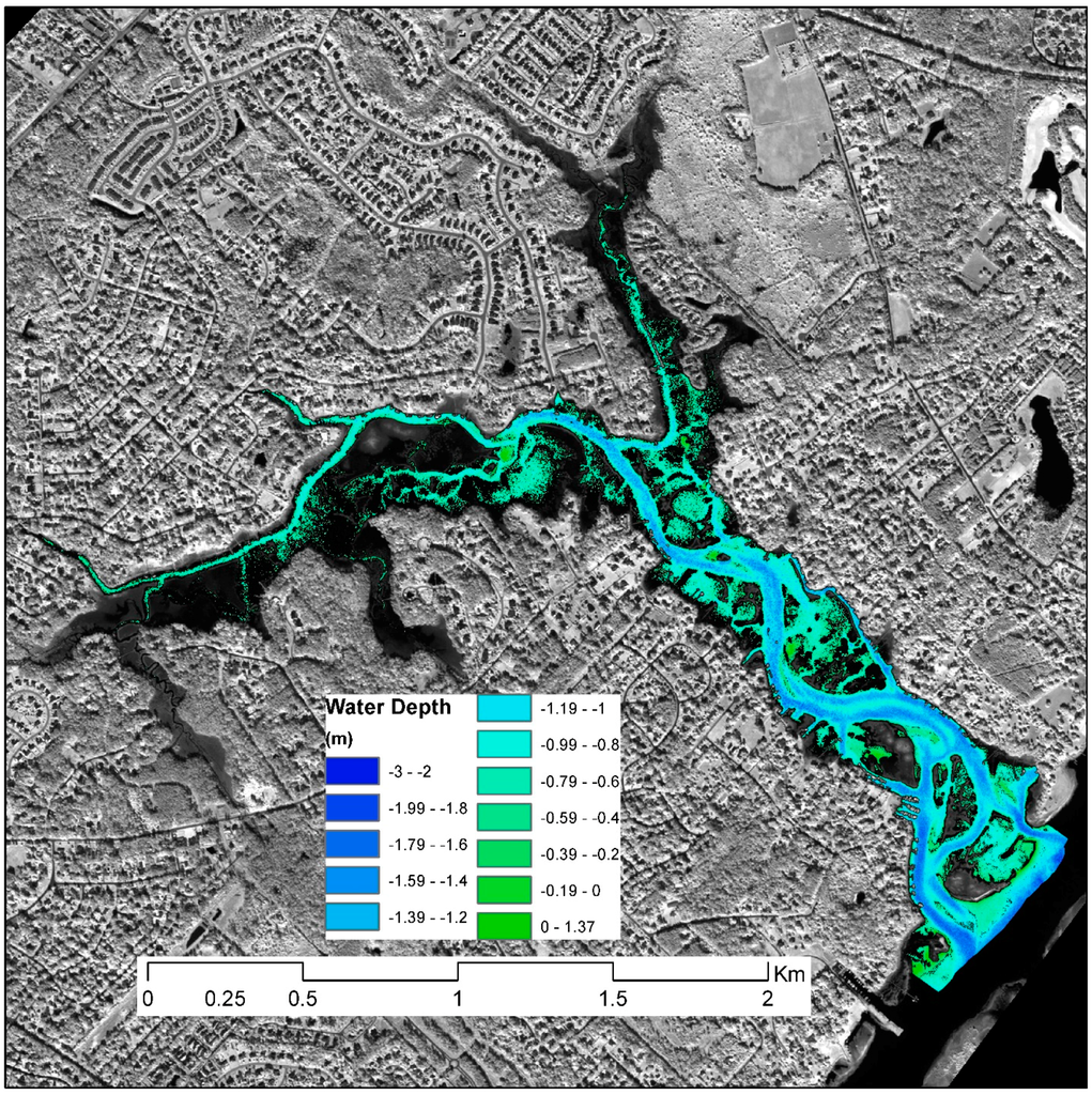
Figure 10.
Derived bathymetry for the Pages Creek study area.
4. Discussion
WV-2’s new spectral bands (coastal blue, yellow, red-edge, and NIR-2) provide more spectral information that is not available in comparable satellites, such as QuickBird, IKONOS, and the new Landsat 8 satellite imagery. Incorporating band ratio indices using WV-2’s new spectral bands and a high-pass convolution filter provided additional information that improved the identification of habitat classes.
Of the nine habitats mapped in this study, oysters and mud had the lowest map accuracy, which was primarily due to being submerged during the time of the image acquisition (tide level was 1.146 m. above MLLW). Usually, it is most desirable to generate maps at low tide; however, it is rare to be able to obtain satellite imagery at ideal times and clear weather. Therefore, the success of the WV-2 imagery to map submerged habitats was one of the main goals of the study. Additionally, ideally the field work should be conducted as close to the date of the remotely-sensed imagery in order to minimize variability as habitats change through time. The extensive field sampling effort enabled high accuracy habitat mapping. Without this large field effort there would probably not be the high level of map accuracy.
The integration of LiDAR derived elevation improved habitat classification especially in the low density cordgrass and black needlerush classes. LiDAR data has become quite widespread, especially along coasts, so these data are very useful in habitat classification especially when merged with satellite imagery. Note that the LiDAR data (2001) used in this study were collected 10 years prior to the acquisition time of WV-2 imagery and may reflect changes in habitat location and water depth. The NCFMP is in its second phase of collecting LiDAR for several counties in southeastern North Carolina, including New Hanover County, and this new LiDAR data should be available soon. Given the fast pace of advancement in LiDAR technology it is clear that these data are providing options for vegetation mapping.
The pan-sharpened WV-2 green and yellow band combination was the most effective for calculating bathymetry. LiDAR was useful in calibrating and assessing shallow water depth. However, additional field data for deeper water had to be collected to effectively convert relative bathymetry to absolute water depths. A total of 117 GRPs were collected, but it is recommended that more GRPs at varying depths and locations should be collected. Although it is difficult to collect water depth measurements, more field work should be conducted and more instruments established to accurately calculate depth. With the tidal environment constantly changing and the nearest NOAA tide gauge not sufficiently close for predicting tide levels, the use of pressure transducers was critical to calibrating water levels in the study area. There are also other methods for deriving bathymetric maps, such multi-beam bathymetry, which is costly due to technical equipment, software, and lengthy time to conduct surveys.
5. Conclusions
Most coastal populations are familiar with the large riverine/estuarine systems, but it is the lesser known and much smaller tidal watersheds that cover a substantial length of the coastline. As coastal populations grow, there is concern that urbanization will lead to poor water quality due to storm-water runoff and increased sedimentation rates, which are detrimental to tidal creek salt marsh and benthic habitats. Accurate and precise high-resolution habitat mapping and bathymetry data are important for managing these complex and highly productive tidal creek habitats [34].
The combination of high spatial and spectral WV-2 imagery, LiDAR derived elevation, extensive field work, robust image processing techniques, and GIS spatial analysis has resulted in highly accurate maps of the tidal creek study area. Few sensors have the ability to distinguish between salt marsh species because of the similar spectral and texture characteristics and small geographic area for each plant species. This study demonstrated that it was possible to map to the species level (such as Spartina alterniflora and Juncus roemerianus) at a very high map accuracy (95%) by using a combination of high spectral resolution WV-2 imagery and LiDAR data. The original 2-m WV-2 image produced higher overall classification accuracy and individual habitat class accuracies than the pan-sharpened and pan-sharpened/atmospherically-corrected images. Therefore, pan-sharpening and atmospheric correction of WV-2 imagery is not needed in this coastal setting.
In the tidal creeks of coastal North Carolina, WV-2 provides excellent spectral information, but at a relatively high cost ($26/km2 academic pricing is approximately $1,000 for this study area). Given the fast pace of advances in satellite technology, the cost of WV-2 imagery will likely decrease as more and more sensors are developed. Interestingly, it was hypothesized that the coastal blue band would be useful for deriving water depth, but this was not the case in this study area.
The methods developed and tested in this study offer a readily repeatable way to derive information about benthic and emergent habitats at a spatial resolution that is significantly higher than historical studies. The field work conducted in this study was rather extensive. Statistically random points were collected for each habitat class and additional GRPs were collected in order to sufficiently calibrate the bathymetry algorithm. Future studies can use the spectral signature information from this study to map adjacent tidal creeks which would reduce the amount of field work that will be necessary.
The final best habitat map was compared with wetland data provided by the local planning agency and only 40% of the wetlands were the same between the two maps. The local planning map was derived from a combination of older aerial photography, state of NC wetlands data, and the National Wetlands Inventory, and was not at the same high-resolution scale as the resulting map from this project. The results of this study demonstrate a valuable method for monitoring tidal creek emergent and submerged habitats that state and local government agencies could use to assess potential long-term changes so that appropriate policies can be developed and implemented in order to minimize detrimental impacts to coastal environments and to monitor changes through time.
Acknowledgments
The authors would like to thank the Department of Earth and Ocean Sciences, University of North Carolina Wilmington, for providing the Trimble RTK equipment and Yvonne Marsan for helping with the GPS software. We would like to thank the reviewers for providing excellent comments and suggestions. Funding support for this publication was provided by the University of North Carolina Wilmington.
Author Contributions
Joanne Halls conceived, designed and planned the research project. Joanne Halls and Kaitlyn Costin conducted the fieldwork. Kaitlyn Costin performed the image processing, statistics, and derivation of bathymetry. Halls wrote the majority of the manuscript and created the figures and tables.
Conflicts of Interest
The authors declare no conflict of interest.
Appendix A
To compare the tide height in Pages Creek with the NOAA tide gauge, the NOAA LiDAR data was converted to mean lower low water (NOAA standard datum) using the NOAA Vdatum tool:
- Download and unzip NOAA Vdatum tool (http://vdatum.noaa.gov/).
- Open tool, select correct datum information for source and target.
- Source: NAVD88 US survey foot height
- Target: MLLW US survey foot height
- Since V-datum does not cover Pages Creek, 10 points were randomly selected off the coast of Wrightsville Beach and Figure Eight Island, imported these points into a spreadsheet, converted the file to ASCII format, containing only ID, latitude and longitude, and elevation columns, with no header. Since elevation is unknown, it was set to zero. Convert the data using mean lower low water (MLLW) datum.
- Calculate the average for the 10 points, 2.57 feet. Use this to convert between NAVD88 and MLLW for Pages Creek.
To derive bathymetry using WorldView-2 imagery, a tide correction must be computed in order to determine the water depth relative to the time the imagery was acquired. First, the time difference between the NOAA tide station and the pressure transducers located in Pages Creek were calculated. The time difference was then used to determine tide height for the Worldview-2 imagery.
The following steps were used to calculate the tide correction:
- Download verified (not modeled) water level from NOAA for the same dates as collected for the pressure transducers (http://tidesandcurrents.noaa.gov/).
- Identify the peaks in the pressure transducer data at both locations and in the NOAA data (Figure A1). Calculate the time differences between peaks and then calculate the average time difference between the NOAA tide gauge and the pressure transducers. For this study area the time difference was 2:04:45.
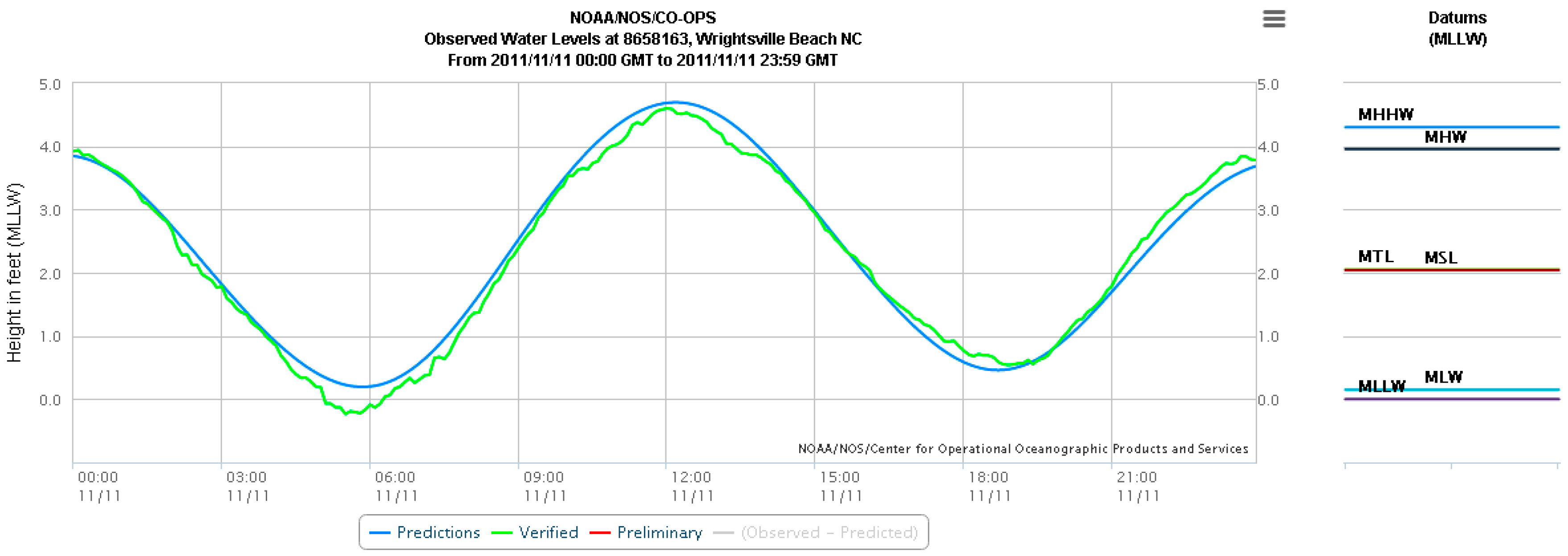
- Using the calculated time difference; look up the NOAA verified water level for the WV-2 imagery acquisition time minus 2:04:45 (Figure A2). Therefore, the WV-2 imagery was acquired at 3.76 feet above mean lower low water.
- Apply the tide difference to LiDAR and GRP data to get the water depth that corresponds to the time the WV-2 imagery was acquired.
- Multiply water depth by −1 to convert to bathymetry.

Figure A1.
Tide heights for the pressure transducers and NOAA tide gauge.
Figure A1.
Tide heights for the pressure transducers and NOAA tide gauge.
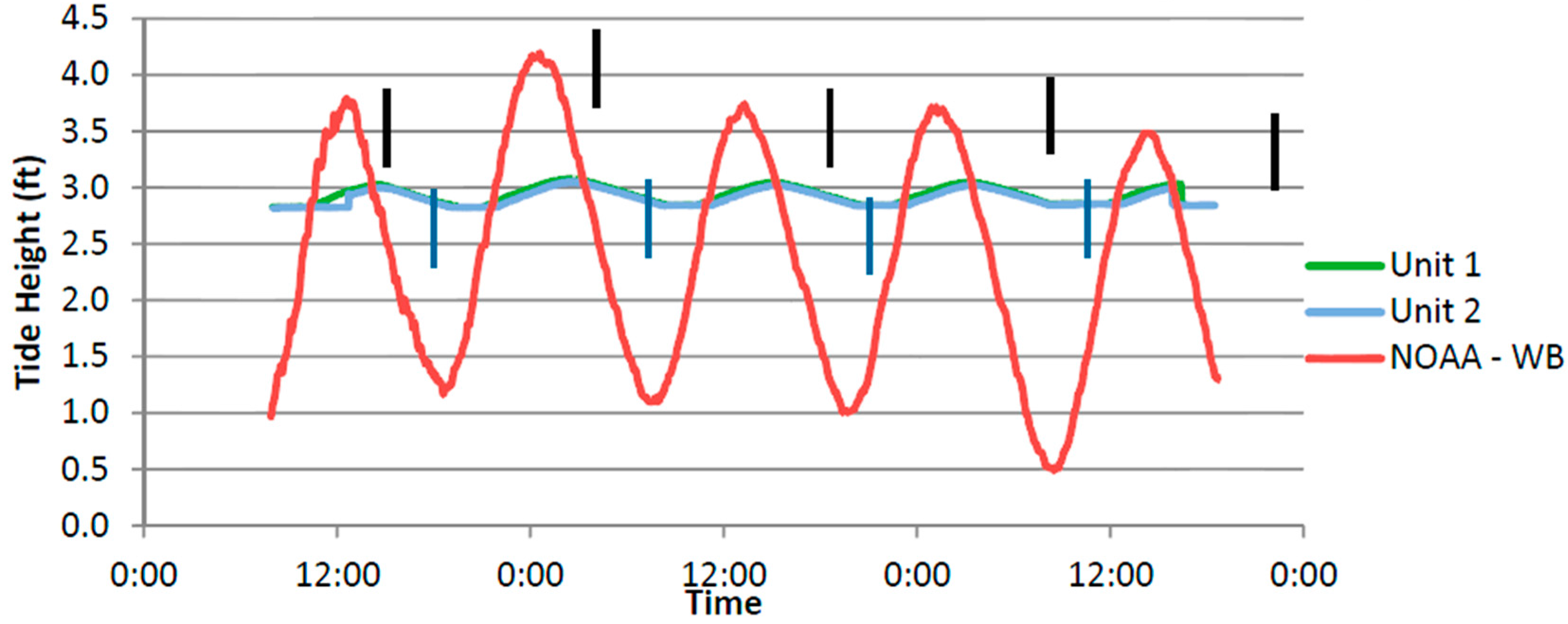
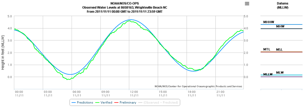
Figure A2.
Verified tide height for adjusted WV-2 imagery acquisition time.
Figure A2.
Verified tide height for adjusted WV-2 imagery acquisition time.
References
- Bricker, S.B.; Clement, C.G.; Pirhalla, D.E.; Orlando, S.P.; Farrow, D. National Estuarine Eutrophication Assessment: Effects of Nutrient Enrichment in the Nation’s Estuaries; NOAA National Ocean Service, Special Projects Office and National Centers for Coastal Ocean Science: Silver Spring, MD, USA, 1999.
- Collin, A.; Hench, J.L. Towards deeper measurements of tropical reefscape structure using the WorldView-2 spaceborne sensor. Remote Sens. 2012, 4, 1425–1447. [Google Scholar] [CrossRef]
- Davis, R.A., Jr.; FitzGerald, D.M. Beaches and Coasts; Blackwell Publishing: Malden, MA, USA, 2004; pp. 263–288. [Google Scholar]
- Bramante, J.F.; Kumaran, R.; Sin, M.T. Multispectral derivation of bathymetry in Singapore’s shallow, turbid waters. Int. J. Remote Sens. 2013, 34, 2070–2088. [Google Scholar] [CrossRef]
- Stumpf, R.; Holderied, K.; Sinclair, M. Determination of water depth with high-resolution satellite imagery over variable bottom types. Limnol. Oceanogr. 2003, 48, 547–556. [Google Scholar] [CrossRef]
- Wiegert, R.G.; Freeman, B.J. Tidal Salt Marshes of the Southeast Atlantic Coastal: A Community Profile; Fish and Wildlife Service, U.S. Department of the Interior: Washington, DC, USA, 1990.
- Mumby, P.J.; Edwards, A.J. Mapping marine environments with IKONOS imagery: Enhanced spatial resolution can deliver greater thematic accuracy. Remote Sens. Environ. 2002, 82, 248–257. [Google Scholar] [CrossRef]
- Wang, L.; Sousa, W.P.; Gong, P.; Biging, G.S. Comparison of IKONOS and Quickbird images for mapping mangrove species on the Caribbean coast of Panama. Remote Sens. Environ. 2004, 91, 432–440. [Google Scholar] [CrossRef]
- Digital Globe. Bathymetry; Technical Note; Digital Globe: Westminster, CO, USA, 2009. [Google Scholar]
- Puetz, A.M.; Lee, K.; Olsen, R.C. Worldivew-2 data simulation and analysis results. Proc. SPIE 2009. [Google Scholar] [CrossRef]
- Matthew, M.W.; Adler-Golden, S.M.; Berk, A.; Felde, G.; Anderson, G.P.; Gorodetzky, D.; Paswaters, S.; Shipper, M. Atmospheric correction of spectral imagery: Evaluation of FLAASH algorithm with AVIRI data. Proc. SPIE 2003. [Google Scholar] [CrossRef]
- Chust, G.; Galparsoro, I.; Borja, A.; Franco, J.; Uriarte, A. Coastal and estuarine habitat mapping, using LiDAR height and intensity and multispectral imagery. Estuar. Coast. Shelf Sci. 2008, 78, 633–643. [Google Scholar] [CrossRef]
- Bork, E.W.; Su, J.U. Integrating LiDAR data and multispectral imagery for enhanced classification of rangeland vegetation: A meta-analysis. Remote Sens. Environ. 2007, 111, 11–24. [Google Scholar] [CrossRef]
- Lee, S.; Shan, J. Combining LiDAR elevation data and IKONOS multispectral imagery for coastal classification mapping. Mar. Geod. 2003, 26, 117–127. [Google Scholar] [CrossRef]
- Bater, C.W.; Coops, N.C. Evaluating error associated with LiDAR-derived DEM interpolation. Comput. Geosci. 2009, 35, 289–300. [Google Scholar] [CrossRef]
- Hladik, C.; Alber, M. Accuracy assessment and correction of a LiDAR-derived salt marsh digital elevation model. Remote Sens. Environ. 2012, 121, 224–235. [Google Scholar] [CrossRef]
- Hladik, C.; Schalles, J.; Alber, M. Salt marsh elevation and habitat mapping using hyperspectral and LiDAR data. Remote Sens. Environ. 2013, 139, 318–330. [Google Scholar] [CrossRef]
- Zlinszky, A.; Mucke, W.; Lehner, H.; Briese, C.; Pfeifer, N. Categorizing wetland vegetation by airborne laser scanning on Lake Balaton and Kis-Balaton, Hungary. Remote Sens. 2012, 4, 1617–1650. [Google Scholar] [CrossRef]
- Kanno, A.; Tanaka, Y.; Shinohara, R.; Kurosawa, A.; Sekine, M. Which spectral band of the Worldview-2 are useful in remote sensing of water depth? A case study of coral reefs. Mar. Geod. 2014, 37, 282–292. [Google Scholar] [CrossRef]
- Lyons, M.; Phinn, S.; Roelfsema, C. Integrating Quickbird multi-spectral satellite and field data: Mapping bathymetry, seagrass cover, seagrass species and change in Moreton Bay, Australia in 2004 and 2007. Remote Sens. 2011, 3, 42–64. [Google Scholar] [CrossRef]
- Madden, C.K. Contribution to Remote Sensing of Shallow Water Depth with the WorldView-2 Yellow Band; Naval Postgraduate School: Monterey, CA, USA, 2011. [Google Scholar]
- Digital Globe. Radiometric Use of Worldview-2 Imagery; Technical Note; Digital Globe: Westminster, CO, USA, 2009. [Google Scholar]
- Mallin, M.; Steffy, E.; McIver, M.; Clay, E. Environmental Quality of Wilmington and New Hanover County Watersheds. CMS Report. 2012. Available online: http://uncw.edu/cms/aelab/Wilmington%20Watersheds/WW%20report%202011.pdf (accessed on 3 April 2016).
- Zhang, Y.; Mishra, R.M. From UNB PanSharp to Fuze Go—The success behind the pan-sharpening algorithm. Int. J. Imag. Data Fusion 2014, 5, 39–53. [Google Scholar] [CrossRef]
- Elsharkawy, A.; Elhabiby, M.; El-Sheimy, N. Quality control on the radiometric calibration of the WoldView-2 data. In Proceedings of the Global Geospatial Conference, Quebec City, Canada, 14–17 May 2012.
- Wolf, A. Using WorldView-2 VIS-NIR MSI Imagery to Support Land Mapping and Feature Extraction Using Normalized Difference Index Ratios; Digital Globe: Westminster, CO, USA, 2010. [Google Scholar]
- Shan, J.; Toth, C.K. Topographic Laser Ranging and Scanning: Principles and Processing; CRC Press: Boca Raton, FL, USA, 2009. [Google Scholar]
- Lyzenga, D.R.; Malinas, N.P.; Tanis, F.J. Multispectral bathymetry using a simple physically based algorithm. IEEE Trans. Geosci. Remote Sens. 2006, 44, 2251–2259. [Google Scholar] [CrossRef]
- Theobald, D.M.; Stevens, D.L.; White, D.; Urquhart, N.C.; Olsen, A.R. Using GIS to generate spatially balanced random survery designs for natural resource applications. Environ. Manag. 2007, 40, 134–146. [Google Scholar] [CrossRef] [PubMed]
- Chen, Z.; Muller-Karger, F.E.; Hu, C. Remote sensing of water clarity in Tampa Bay. Remote Sens. Environ. 2007, 109, 249–259. [Google Scholar] [CrossRef]
- Chen, D.; Stow, D. The effect of training strategies on supervised classification at different spatial resolutions. Photogramm. Eng. Remote Sens. 2002, 68, 1155–1161. [Google Scholar]
- Vahtmae, E.; Kutser, T. Classifying the Baltic Sea shallow water habitats using image-based and spectral library methods. Remote Sens. 2013, 5, 2451–2474. [Google Scholar] [CrossRef]
- Congalton, R.G.; Green, K. Assessing the Accuracy of Remotely Sensed Data: Principles and Practices, 2nd ed.; CRC Press: Boca Raton, FL, USA, 2009. [Google Scholar]
- Mutanga, O.; Adam, E.; Moses, A.O. High density biomass estimation for wetland vegetation using WorldView-2 imagery and random forest regression algorithm. Int. J. Appl. Earth Obs. Geoinf. 2012, 18, 399–406. [Google Scholar] [CrossRef]


© 2016 by the authors; licensee MDPI, Basel, Switzerland. This article is an open access article distributed under the terms and conditions of the Creative Commons Attribution (CC-BY) license (http://creativecommons.org/licenses/by/4.0/).