Mapping Above-Ground Biomass by Integrating Optical and SAR Imagery: A Case Study of Xixi National Wetland Park, China

Abstract

Wetlands are important ecosystems as they are known as the “kidney of the earth”. Particularly, urban wetlands play an important role in providing both natural and social beneficial services. However, urban wetlands are suffering from various human impacts, such as excessive land use conversion, air and water pollution, especially those in developing countries undergoing rapid industrialization and urbanization. Therefore, it is of great necessity to derive timely biomass information for optimal design, management and protection of urban wetlands. In this paper, we develop a set of models for estimating above ground biomass (AGB) in Xixi National Wetland Park in Hangzhou, China by using optical images and Synthetic Aperture Radar (SAR) images. A series of vegetation indices (VIs) derived from optical data is introduced along with spectral data. The modeling methods consist of (1) curve estimation; (2) linear regression for multivariable model; (3) Back Propagation Neural Network (BPNN) modeling. Curve estimation is a combination of linear and nonlinear regressions. It is applied to generate AGB models from a single variable including Normalized Difference Vegetation Index (NDVI) and radar backscatter coefficient. The models are then compared via three accuracy metrics. According to the results, SAR models generally show better accuracy than optical models and BPNN models show the greatest accuracy among all the models. The BPNN model from the combination of Terra Advanced Spaceborne Thermal Emission and Reflection Radiometer (ASTER) and European Remote-Sensing Satellite-2 (ERS-2) SAR (Synthetic Aperture Radar) image has the least root mean square (RMSE, 0.396 kg/m²), least mean absolute error (MAE, 0.256 kg/m²) and the greatest correlation coefficient (0.974). The results indicate that AGB can be estimated by integrating optical and SAR imagery. Four maps of AGB are derived to illustrate the distribution of AGB in the study area. The total AGB in the study area is estimated to be between 165,000 and 210,000 kg/m².

1. Introduction

Wetlands are important ecosystems because they play a vital role in environmental function [1,2]. Thus, mapping various biophysical parameters of wetlands has attracted interest in a variety of ecological, environmental studies in recent years, including their distribution, leaf area index, biomass, etc. [3,4,5]. Above ground biomass (AGB) has been frequently analyzed among these parameters, which is defined as the total biomass of foliage and woody components of a vegetation canopy above the ground level [6]. The total amount of AGB is not only a key index in measuring the health of the wetland ecosystem [7] but also an indicator, closely related to the United Nations Reducing Emissions from Deforestation and Forest Degradation (REDD) program, as well as the international negotiations on climate change [8]. Urban wetlands refer to natural and artificial wetlands distributed in urban areas [9]. These urban wetlands play an important role in providing not only ecological services but also social services such as cultural benefits [10,11]. However, urban wetlands are suffering from various human impacts, such as excessive land use conversion, air and water pollution [12], especially those in developing countries at a rapid industrialization and urbanization stage [13]. Therefore, it is of great necessity to derive timely AGB information for optimal design, management and protection of urban wetlands.

Different methods have been developed for mapping wetlands. For example, local-scale field measurements (e.g., Diameter at Breast Height, DBH) are integral to estimate wetland AGB using allometric equations [6]. In spite of its effectiveness, field measurements are expensive and time-consuming [8] and sometimes inapplicable in some protected areas. In contrast, satellite remote sensing images, ranging from coarse to fine spatial resolution, have been increasingly used for mapping wetland AGB [14]. Due to its sensitivity for detecting wetland AGB, Normalized Difference Vegetation Index (NDVI) has been used for key input information to build models for AGB calculation in a number of studies [15]. Moreau et al. [16] built simple kernel-driven models based on bidirectional reflectance distribution function normalized NDVI for estimating Andean bofedal and totora wetland grasses using National Oceanic and Atmospheric Administration/Advanced Very High Resolution Radiometer (NOAA/AVHRR) imagery. Zhao et al. [17] monitored rapid vegetation succession in estuarine wetlands in the Yangtze River Delta area using various vegetation indices (VIs) derived from Moderate Resolution Imaging Spectroradiometer (MODIS) imagery. Xie et al. [18] compared different regression models by combining four types of VIs and found that models that combined Difference Vegetation Index (DVI) had the best performance for estimating the AGB of the wetland bulrush in the Qaidam Basin, China. Chen et al. [19] analyzed the error propagation associated with scaling foliage biomass from field measurements to Landsat, MODIS and AVHRR data over a northern Canadian national park. In these studies, Landsat Thematic Mapper/Enhanced Thematic Mapper Plus (TM/ETM+) imagery is the most widely used optical imagery for mapping wetlands because of the historical Landsat archive used with an appropriate resolution. High spatial resolution images such as IKONOS, Quickbird, were also used for mapping wetland biomass [20,21,22].

On the contrary, Synthetic Aperture Radar (SAR) imagery provides unique and valuable information on wetland biophysical parameters by exploiting the particular sensitivity of radar backscatter signal to the AGB [23,24]. For wetlands located in the tropical and sub-tropic regions (e.g., Southeast China), the presence of clouds and the long rainy season limit the use of optical satellite imagery for wetland studies. While SAR allows day-and-night and all-weather imaging, an ideal alternative data source for monitoring and mapping wetlands in these areas [25]. Envisat Advanced Synthetic Aperture Radar (ASAR) imagery is one of the most frequently used SAR dataset for AGB retrieval. For instance, the potential of Envisat ASAR imagery for woody AGB assessment was explored in a national park in India [26]; AGB and other ecosystem information was retrieved from ERS-2 SAR and Envisat ASAR polarized data for wetland management in Poland [27]. Other SAR sensors have also been applied in the AGB estimation, such as Advanced Land Observing Satellite Phased Array type L-band Synthetic Aperture Radar (ALOS PalSAR) [28] and airborne OrbiSAR-1 [29]. However, a series of studies shows that the relationship between AGB and backscatter from L-band SAR varies as the AGB level changes. However this does not occur where AGB is greater than 15 kg/m² but does exist at the lower level of biomass [30,31,32]. Furthermore, efforts have been made to combine optical and radar remote sensing imagery for AGB mapping [4]. Some studies estimated tropical forest AGB by combining Japanese Earth Resources Satellite (JERS-1) and Landsat TM data [33], while others compared models between AGB and NDVI, assessing the backscatter models for estimating mangrove AGB and finding that radar imagery gave significant improvement [34].

This study tries to address the following issues for estimating and mapping AGB in urban wetlands. First, AGB reflectance of different plant species varies greatly [35] which may result in the inaccurate mapping of wetland biomass. Second, the remote-sensing based AGB estimation has not been reported for urban wetlands in Southeast China, such as Xixi National Wetland Park. In terms of the AGB analysis of the wetlands in Southeast China, most studies focused on those wetlands (not urban wetlands) located in Poyang Lake [7,36]. Therefore, two primary goals of this study include: (1) to implement AGB estimation by integrating widely used optical and SAR imagery in Xixi National Wetland Park; (2) to compare the performance of various AGB estimation models, including linear, nonlinear regression models and the BPNN model [37,38].

2. Study Site and Materials

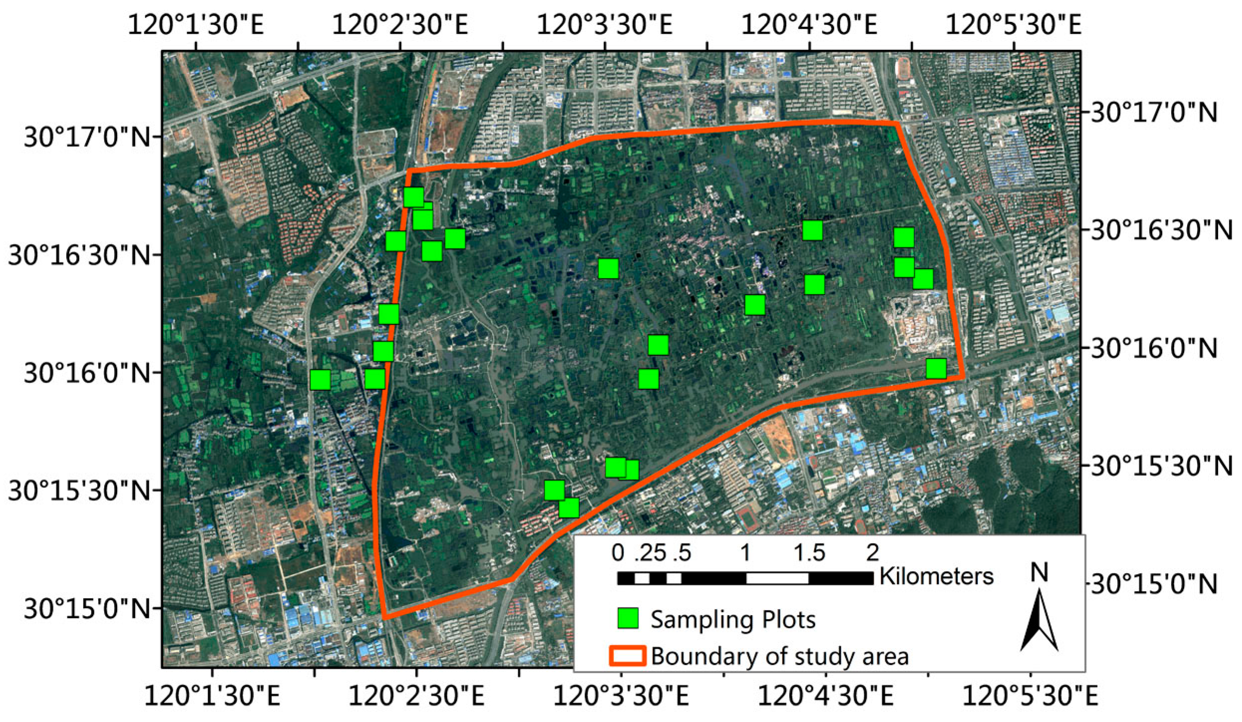
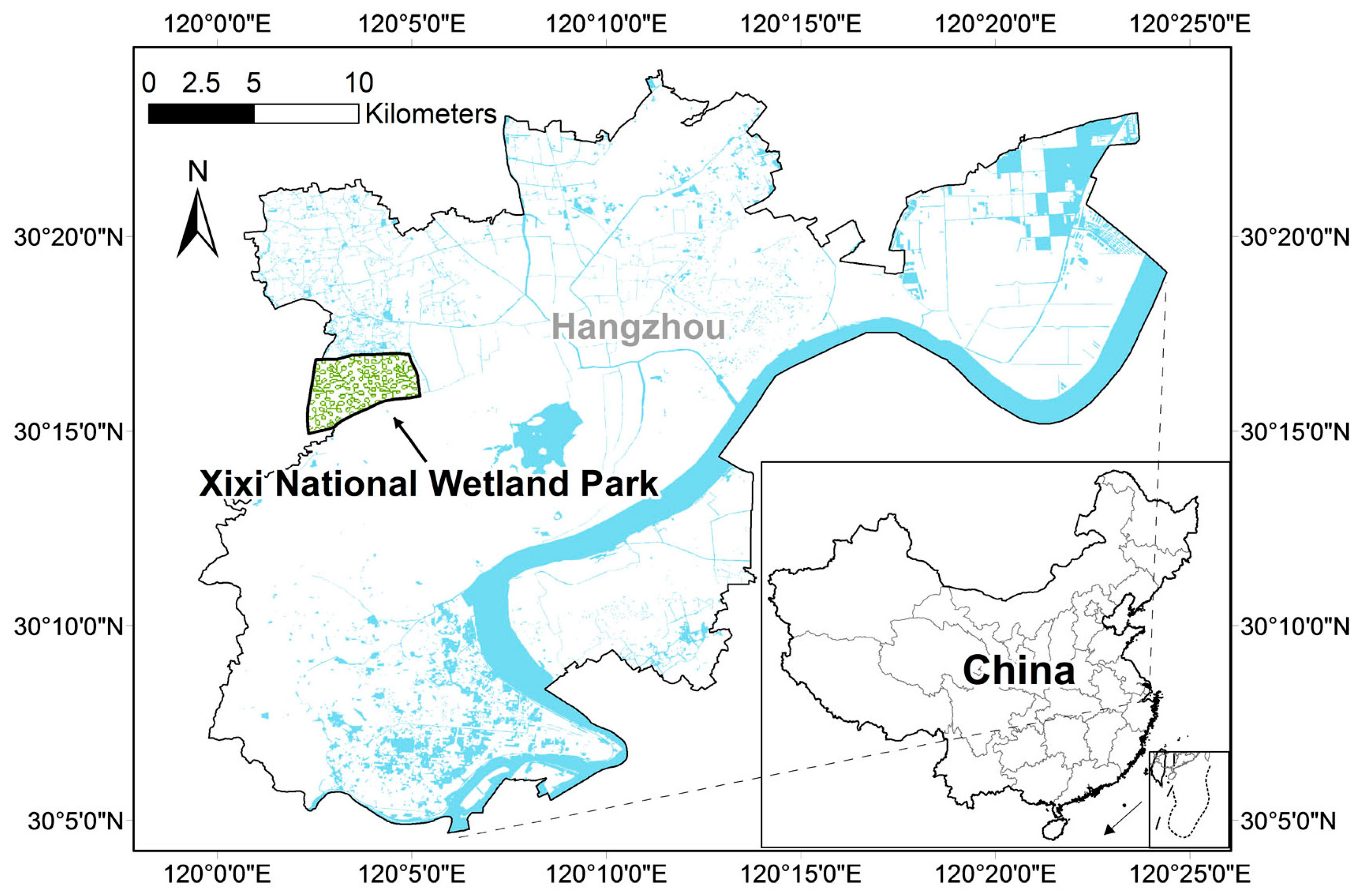
2.1. Study Site

With an approximate area of 11 km², Xixi National Wetland Park is located in Southeast China (30°14′57.1″~30°16′59.9″N, 120°02′20.6″~120°05′12.3″E) (see Figure 1). It is one of the first National Wetland Parks in China (approved in 2005). The park is located within an urban wetland called “Xixi Wetland”. Due to a subtropical monsoon climate with an annual precipitation of approximate 1400 mm, vascular plants dominate in this area. It is estimated that there are 119 vascular species belonging to 103 genera and 44 families, of which 50 are wetland plants [39,40].

2.2. Field Sampling

Since the study site is a National Wetland Park, destructive sampling and weighing of dried vegetation components in the park is prohibited by law. Alternatively, destructive sampling can be carried out in an area outside the park. This public area contains some wetlands adjacent to the Xixi National Wetland Park enabling destructive sampling within a comparable ecological landscape with similar vegetation species. Figure 2 is a true-color map from Google Earth^® showing the locations of AGB plots.

Field estimates of AGB were conducted in different ways for herbaceous vegetation, shrub and for trees with large DBH (i.e., 10 cm in diameter or larger). A total of 24 plots were chosen as the sampling area either inside or outside the National Wetland Park. Some sampling plots cover more than 1 pixel area. Each pixel covers a 12.5 m × 12.5 m square on the land. The field inventory was acquired from April to May 2009 with the following procedure:

Step 1: for herbaceous vegetation and shrubs, a series of 0.5 m × 0.5 m small parcels were chosen to represent various vegetation coverage, vegetation type and vegetation height. The vegetation was cut and taken back to laboratory for measuring dry weight as AGB.

Step 2: for trees with large DBH, tree species were recorded and their DBH and tree heights were measured. Dry AGB was estimated using existing allometry [41,42,43].

Step 3: the coordinates of sampling sites were recorded simultaneously using handheld global positioning system (GPS) devices.

Step 4: the coordinates of sampling sites were imported to an ArcGIS^® dataset and the land cover in each plot was identified through Google Earth^® high resolution images and the field survey.

Step 5: the AGB measured in Step 1 and Step 2 was related to sites in the ArcGIS^® dataset, so AGB within each 12.5 m × 12.5 m area was estimated.

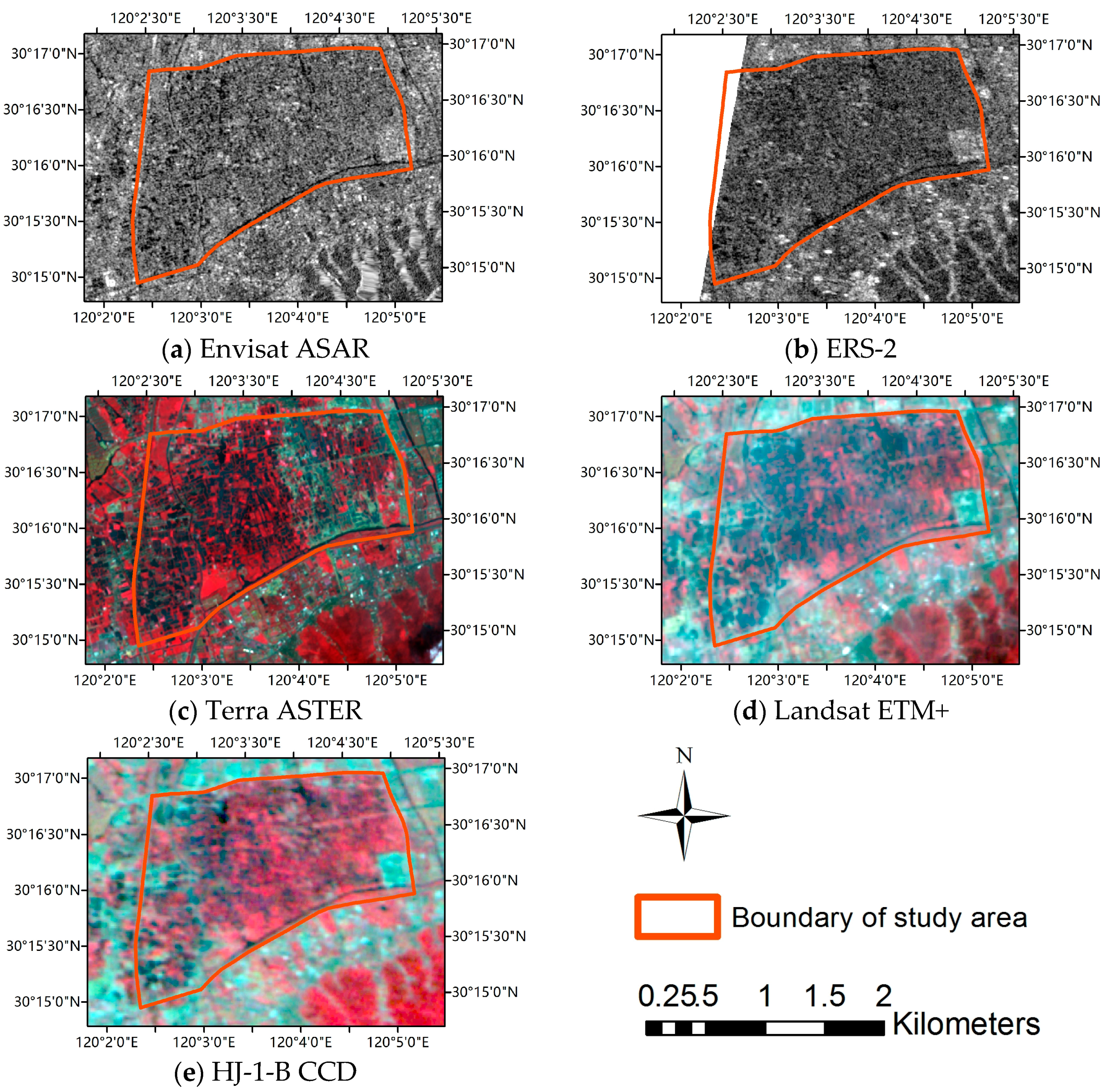
2.3. Remote Sensing Imagery Acquisition and Pre-Processing

All remote sensing images used in this study are listed in

Table 1. Remote Sensing Images Used in This Study.

Sensor Type	Data Type	Pass	Acquisition Date
Radar	Envisat ASAR HH/VV	Ascending	17 August 2009
Radar	ERS-2 SAR VV	Descending	22 March 2009
Optical	Terra ASTER	Descending	16 March 2009
Optical	Landsat ETM+	Descending	11 April 2009
Optical	HJ-1-B CCD	Descending	21 April 2009

and Figure 3. In terms of optical images, data is from Chinese HJ-1-B, Landsat and Terra ASTER, with a nearly coincident acquisition date and similar spectral range. Particularly, there are four optical bands with the HJ-1-B imagery, which approximately corresponds to the first four bands of Landsat 7 ETM+ imagery (blue, green, red and infrared bands, respectively). More details about the HJ-1-B optical images can be found in Wang et al. [44]. Terra ASTER, Landsat ETM+ and HJ-1-B images were used for calculating various VIs. While the scanner line corrector of Landsat 7 failed in May 2003, it has almost no impact on this research because our study site is located in a non-gapped region of the Landsat ETM+ imagery. The original digital numbers (DN) of these images were calibrated to at-satellite reflectance in ENVI 4.8^®.

In terms of SAR imagery, we used Envisat ASAR and ERS-2 SAR, which are C-band microwave backscatter data. The Envisat ASAR imagery was acquired in an alternating polarization mode, which is VV/HH polarized (vertically transmitted and vertically received/horizontally transmitted and horizontally received polarization of backscatter). We searched Envisat ASAR and ERS-2 SAR imagery in the catalogues of ESA’s Earth Observation data products. ERS-2 SAR images are all VV polarized; and there are more Envisat ASAR VV polarized images than any multi-polarization such as VV/HH. Several terrain and SAR parameter interactions influence the backscatter coefficient, therefore pre-processing is necessary to get SAR intensity images that represent the radar backscatter from the land surface. Envisat ASAR and ERS-2 SAR imagery were pre-processed in Next European Space Agency (ESA) SAR Toolbox-4C-1.1 (NEST) radiometric calibration and terrain correction using Shuttle Radar Topography Mission (SRTM) data. The processed output data were ortho-rectified backscatter data (in dB) at a spatial resolution of 12.5 m. For further analysis, all optical images and VIs data were resampled to a spatial resolution of 12.5 m using cubic convolution interpolation.

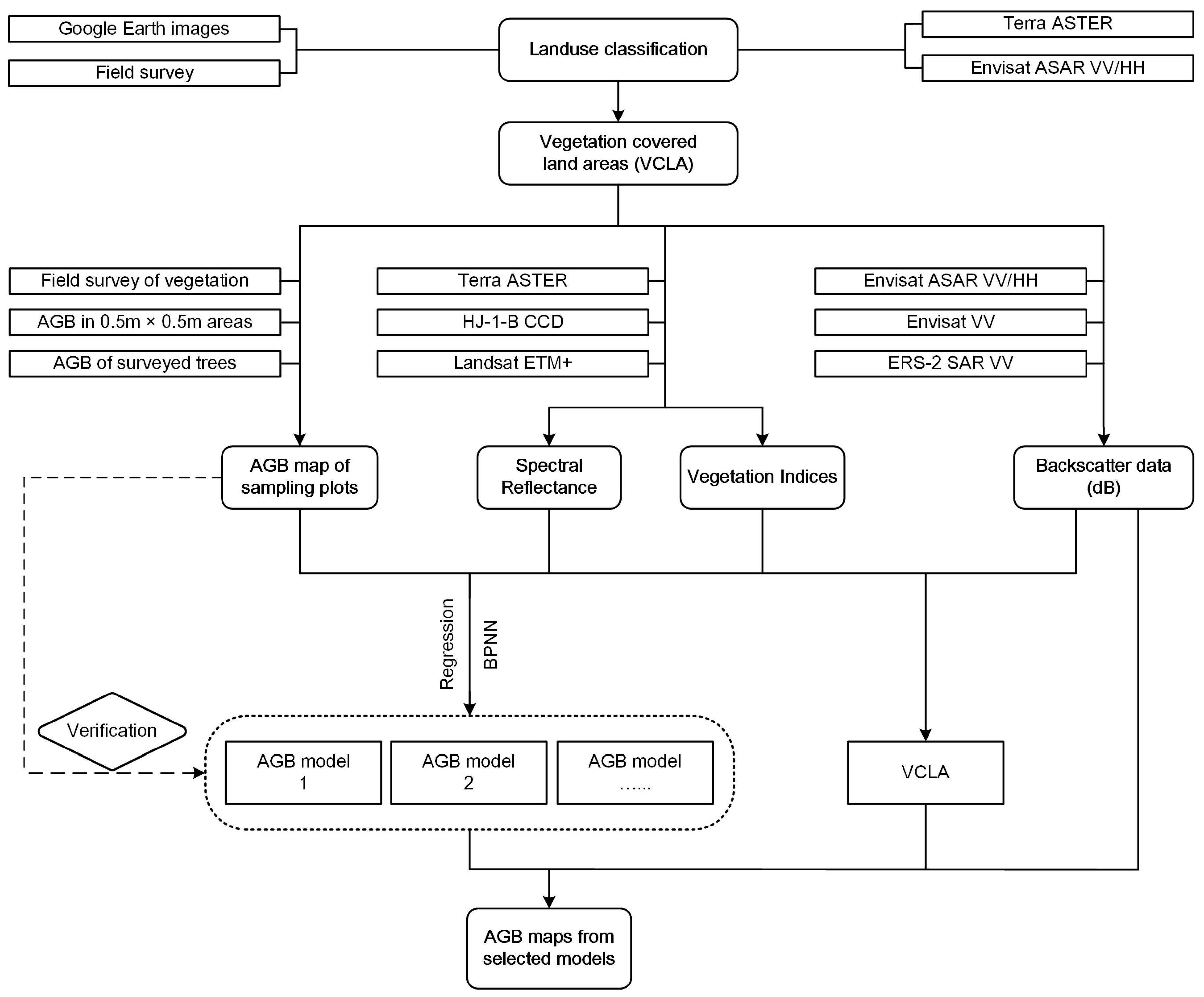
3. Methods

The flowchart of the whole study is shown in Figure 4.

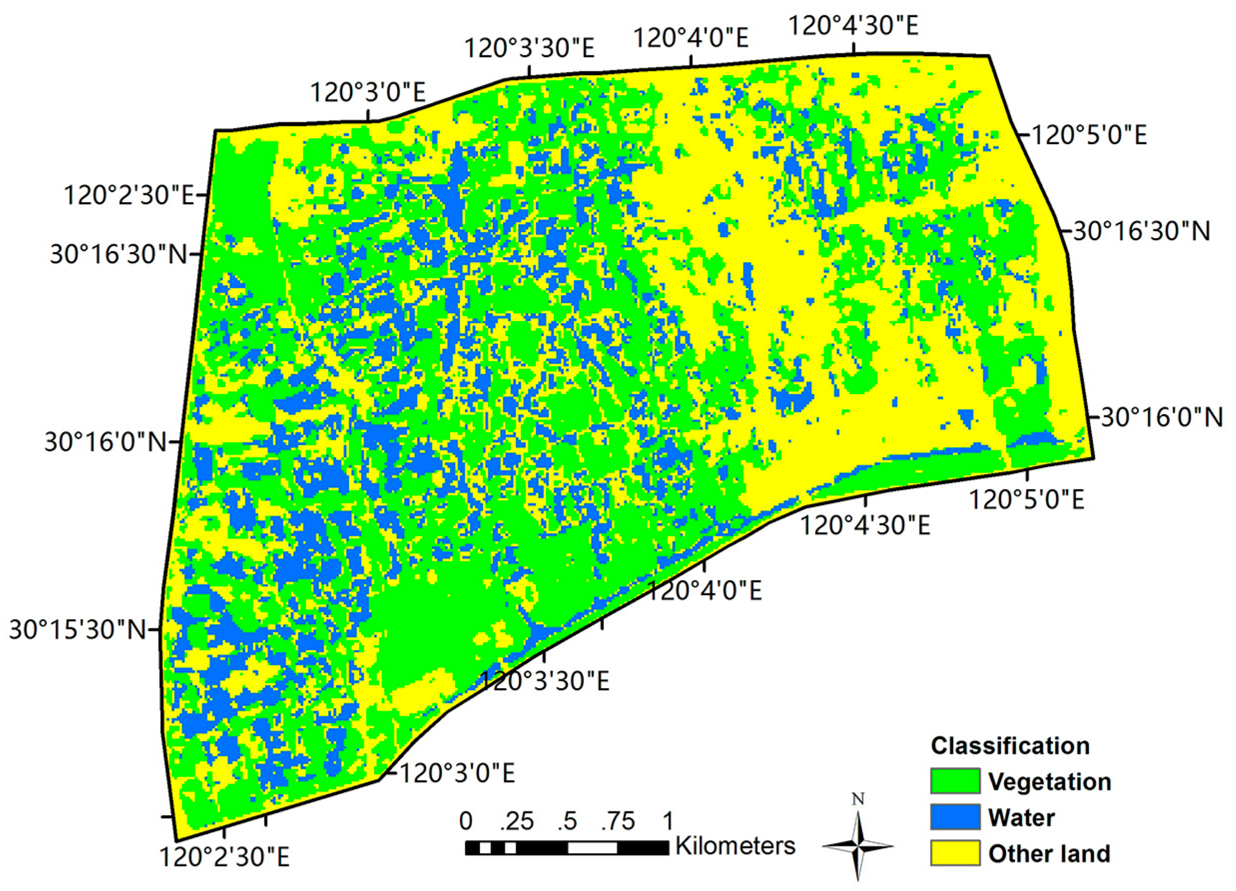
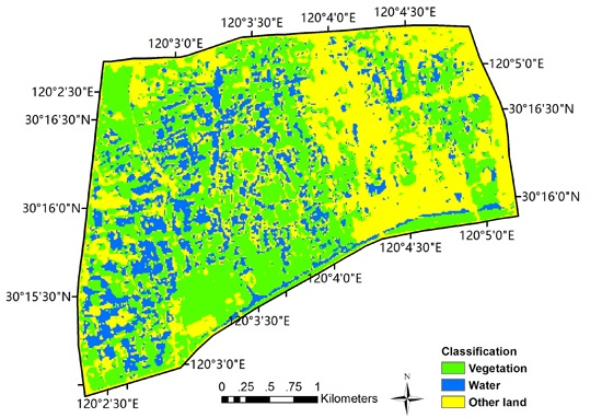
3.1. Classification for Vegetation Covered Land Area

The potential models calculate AGB in vegetation covered land areas (VCLA), not in bare lands, water, or any other areas where AGB is 0. The VCLA should be retrieved prior to applying the biomass estimation models. This study used a supervised classification for VCLA in ENVI 4.8^® based on selection of region of interest (ROI).

(1)

Terra ASTER and Envisat ASAR images were input for the classification. We used both optical and SAR images to improve the classification.

(2)

The ROI was selected with the help of high resolution imagery in Google Earth^®, containing vegetation, water and other land cover. As for each type of land cover, we selected 12 typical ROIs, where each ROI covered multiple pixels.

(3)

The Maximum Likelihood classifier in ENVI 4.8^® was used for the supervised classification. The VCLA were retrieved and the classification accuracy was examined via user’s accuracy and producer’s accuracy.

3.2. Calculations of Relevant Variables

3.2.1. VIs Calculation

In order to improve the AGB estimation models, VIs were calculated to characterize vegetation and to distinguish tree canopy area and cropland/grassland [45,46,47,48,49]. These VIs include NDVI, Global Environment Monitoring Index (GEMI) [50], Transformed Normalized Difference Vegetation Index (TNDVI) [51] and Renormalized Difference Vegetation Index (RDVI) [52]. The formulas of these VIs are given by:

$$NDVI=\frac{NIR-R}{NIR+R}$$

(1)

$$GEMI=\frac{\mathsf{\eta }(1-0.25\mathsf{\eta })-(R-0.125)}{1-R}$$

(2)

$$\mathsf{\eta }=\frac{2(NI{R}^2-R^2)+1.5NIR+0.5R}{NIR+R+0.5}$$

(3)

$$RDVI=\frac{NIR-R}{\sqrt{NIR+R}}$$

(4)

$$TNDVI=\sqrt{NDVI+0.5}$$

(5)

where $R$ and $NIR$ are the reflectance of red and near infrared band, respectively. In the analysis, apparent reflectance was used instead as it was more practical [53,54].

Although these VIs are derived from both red and near infrared bands, their performance may be different: GEMI, RDVI and NDVI may show better capability in urban areas, while TNDVI may be better in distinguishing tree canopy from other vegetation, such as grasslands or shrubs [48]. Potential multicollinearity of these VIs will be discussed in the Result section.

3.2.2. Accuracy Assessment

Three accuracy metrics were employed to assess the accuracy of the biomass estimates, including Pearson’s correlation coefficient, root mean square error (RMSE) and mean absolute error (MAE). These metrics can be expressed as follows [55]:

$$r=\frac{{\mathsf{\sigma }}_{xy}{}^2}{{\mathsf{\sigma }}_x{\mathsf{\sigma }}_y}=\frac{{\displaystyle \sum (x-\overline{x})(y-\overline{y})}}{\sqrt{{{\displaystyle \sum (x-\overline{x})}}^2}\cdot \sqrt{{{\displaystyle \sum (y-\overline{y})}}^2}}$$

(6)

where r is Pearson’s correlation coefficient; $x$, $y$ are the real and predicted AGB in this study, respectively; $\overline{x}$, $\overline{y}$ are their mean values.

$$RMSE=\sqrt{\frac{1}{n}{\displaystyle {\sum }_{i=1}^n{(B_i-{\widehat{B}}_i)}^2}}$$

(7)

$$MAE=\frac{1}{n}{\displaystyle {\sum }_{i=1}^n|B_i-{\widehat{B}}_i|}$$

(8)

where ${\widehat{B}}_i$ is the estimated AGB for pixel i; $B_i$ is the actual biomass of pixel retrieved from field sampling and n is the total number of field sampling pixels.

3.3. Optical-Imagery-Only Models

The modeling method used for optical-imagery-only models in this analysis can be classified in three categories: (1) simple regression; (2) multivariable linear regression; (3) BPNN models.

(1)

Simple regression models. They include the usage of both linear and nonlinear models with single independent data. We generated linear and nonlinear regression models using Curve Estimation in IBM SPSS Statistics 20^® (SPSS 20). As NDVI is the most widely used vegetation index, and previous biomass models are mainly based on NDVI, it was used as the only independent variable in the curve estimation.

(2)

Multivariable linear regression models. The independent variables include each type of optical remote sensing spectral reflectance and the derived VIs. Ordinary least square (OLS) regression method was applied to select independent variables in SPSS 20 with a p-value equal to or less than 0.05. Variance Inflation Factor (VIF) was calculated to evaluate the potential multicollinearity problem.

(3)

BPNN models. BPNN is one of the most popular neural networks method and is an excellent nonlinear fit theory, minimizing a global error between predicted outputs and measured values and used in many remote sensing studies [56,57]. The independent variables include spectral reflectance and VIs. In this step, part of sampling data was used to generate BPNN models for estimating AGB, whereas the rest is used for testing the model accuracy.

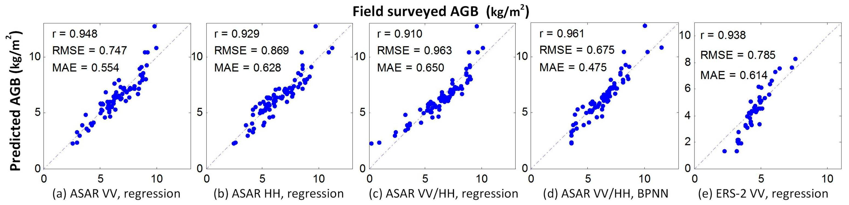
3.4. SAR-Only Models

The modeling method used for SAR-only models is similar to that of optical-imagery-only models and can also be classified in three categories: (1) simple regression; (2) multivariable linear regression; (3) BPNN models.

(1)

Simple regression models. They include the usage of both linear and nonlinear models with single independent data. The independent data is VV or HH polarized microwave backscatter data. We also generated linear and nonlinear regression models using Curve Estimation in SPSS 20.

(2)

Multivariable linear regression models. The independent variables include Envisat ASAR HH/VV data. OLS regression method was also applied to select independent variables in SPSS 20 with a p-value equal to or less than 0.05. VIF was calculated to evaluate the potential multicollinearity.

(3)

BPNN models. The independent variables include microwave backscatter data (${\mathsf{\sigma }}_{VV}^0$, ${\mathsf{\sigma }}_{HH}^0$). Also in this step, part of sampling data is used to generate models, whereas the rest is used for testing the model accuracy.

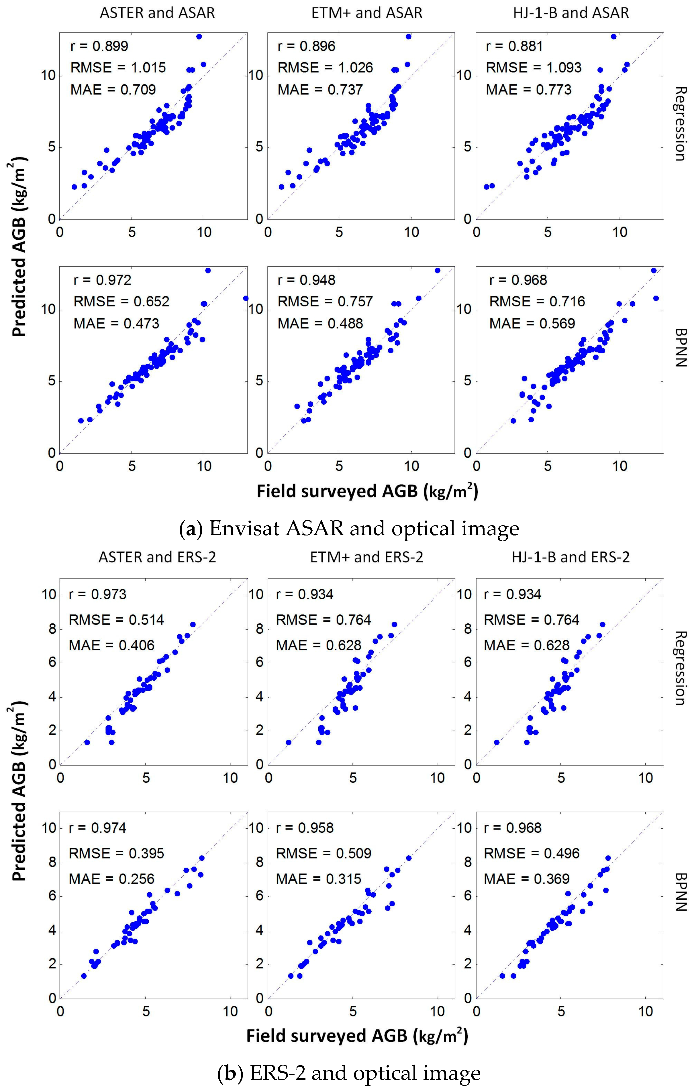
3.5. Combination Models Using Spectral Reflectance and SAR Data

Similarly, the modeling method used in this analysis can be classified into 2 categories: (1) multivariable linear regression; (2) BPNN models.

(1)

Multivariable linear regression models. The independent variables include Envisat ASAR imagery and VIs. OLS regression method was applied to select independent variables in SPSS 20 with a p-value equal to or less than 0.05. VIF was also calculated to evaluate the potential multicollinearity.

(2)

BPNN models. The independent variables include a combination of spectral reflectance, VIs and microwave backscatter data (${\mathsf{\sigma }}_{VV}^0$, ${\mathsf{\sigma }}_{HH}^0$). In this step, part of sampling data is used to generate models, whereas the rest is used for testing the model accuracy.

The model with the largest coefficient of determination (R²) was selected as the best estimation model among all models, by which a map of AGB is derived for our study area.

4. Results

4.1. Classification for Vegetation Covered Areas

In this analysis, SAR and optical imagery had important roles in AGB estimation due to: (1) retrieval of VCLA; (2) biomass modeling and estimation.

Vegetation covered areas contain VCLA and water areas covered by herbaceous plants in the study area. These herbaceous plants were omitted due to the trees and shrubs at much higher AGB level. In addition, the biomass of underwater plants was not considered in this AGB study. Hence, VCLA is retrieved for further study. Spectral data from optical imagery and the derived VIs information have shown capability in retrieving vegetation covered areas [49]. However, VCLA have shown similar characteristics in NDVI maps or false color composite image with water areas covered by herbaceous plants.

Meanwhile, the backscatter data from SAR images in water covered areas is different from VCLA, thus it is more capable of distinguishing these areas from VCLA using SAR data. The land cover in urban wetland is more complicated than in other wetlands. Looking at Google Earth^® images, some areas with high radar backscatter coefficient were buildings or parking lots with cars in the Xixi National Wetland Park. In some of these areas, the backscatter coefficient is similar to vegetation cover. These would lead to a lower accuracy in classification for VCLA without optical remote sensing data.

Consequently, supervised classification for VCLA is fulfilled combining Google Earth^® images, ERS-2 SAR and Terra ASTER images (Figure 5). The Pair Separation value in ENVI 4.8^® between vegetation areas and other types of land cover are all greater than 1.95. For instance, water area and other land cover (including bare land, road and buildings) is 1.9682, comparing to 1.9620 using Terra ASTER data with the same region of interest (ROI) data. We selected some other samples for accuracy assessment: the user’s accuracy of vegetation covered areas is 96.50% and the producer’s accuracy is 97.41%.

4.2. Models and Predictions

In this section, a set of regression models are listed for predicting AGB (

Table 2. Regression Models for Estimating AGB in Xixi National Wetland Park from Spectral Reflectance, VIs and Radar Backscatter Data. Independent Variables are Selected Using Regression Method, $p\le 0.05$; and R² is the Adjusted Coefficient of Determination. B and R Represent the Blue and Red Band in Optical Images, Respectively. Models Marked with “*” Have Greater VIF Values (3 < VIF < 5).

(a) Optical-Only Models
Input		AGB Model (kg/m2)	R2	Significance	VIF
Terra ASTER	NDVI	$AGB=2.245\times e^{5.036\times \text{NDVI}}$	0.775	NDVI: 0.000	/
	Spectral reflectance and VIs	$AGB=31.692\times NDVI+0.165$	0.642	NDVI: 0.000	/
Landsat ETM+	NDVI	$AGB=1.041\times e^{6.060\times \text{NDVI}}$	0.664	NDVI: 0.000	/
	Spectral reflectance and VIs	$AGB=38.318\times NDVI-4.725$	0.559	NDVI: 0.000	/
HJ-1-B CCD	NDVI	$AGB=0.823\times e^{6.777\times \text{NDVI}}$	0.699	NDVI: 0.000	/
	Spectral reflectance and VIs	$AGB=0.438\times \text{NIR}-12.006$	0.548	NIR: 0.000	/
(b) SAR-only models
Input		AGB model (kg/m2)	R2	Significance	VIF
Envisat ASAR	${\mathsf{\sigma }}_{VV}^0$	$AGB=17.469\times e^{0.141\times {\mathsf{\sigma }}_{VV}^0}$	0.874	${\mathsf{\sigma }}_{VV}^0$: 0.000	/
	${\mathsf{\sigma }}_{HH}^0$	$AGB=17.303\times e^{0.136\times {\mathsf{\sigma }}_{HH}^0}$	0.861	${\mathsf{\sigma }}_{HH}^0$: 0.000	/
	${\mathsf{\sigma }}_{VV}^0$, ${\mathsf{\sigma }}_{HH}^0$	$AGB=0.541\times {\mathsf{\sigma }}_{VV}^0+0.408\times {\mathsf{\sigma }}_{HH}^0+13.530$	0.823	${\mathsf{\sigma }}_{VV}^0$: 0.000	${\mathsf{\sigma }}_{VV}^0$: 4.868
				${\mathsf{\sigma }}_{HH}^0$: 0.000	${\mathsf{\sigma }}_{HH}^0$: 4.868
ERS-2	${\mathsf{\sigma }}_{VV}^0$	$AGB=25.534\times e^{0.120\times {\mathsf{\sigma }}_{VV}^0}$	0.871	${\mathsf{\sigma }}_{VV}^0$: 0.000	/
(c) Envisat ASAR and optical models
Input		AGB model (kg/m2)	R2	Significance	VIF
Envisat ASAR		$AGB=0.763\times {\mathsf{\sigma }}_{VV}^0+12.630\times RDVI+9.014$	0.806	${\mathsf{\sigma }}_{VV}^0$: 0.000	${\mathsf{\sigma }}_{VV}^0$: 2.853
Terra ASTER				RDVI: 0.040	RDVI: 2.853
Envisat ASAR, Landsat ETM+		$AGB=0.831\times {\mathsf{\sigma }}_{VV}^0+12.026\times GEMI+7.288$	0.807	${\mathsf{\sigma }}_{VV}^0$: 0.000	${\mathsf{\sigma }}_{VV}^0$: 2.117
				GEMI: 0.039	GEMI: 2.117
Envisat ASAR		$AGB=0.933\times {\mathsf{\sigma }}_{HH}^0-3.950\times RDVI+14.744$	0.842	${\mathsf{\sigma }}_{HH}^0$: 0.000	${\mathsf{\sigma }}_{HH}^0$: 2.136
HJ-1-B CCD				RDVI: 0.047	RDVI: 2.519
(d) ERS-2 and optical models
Input		AGB model (kg/m2)	R2	Significance	VIF
ERS-2		$AGB=0.346\times {\mathsf{\sigma }}_{VV}^0+18.104\times RDVI+5.828$	0.870	${\mathsf{\sigma }}_{VV}^0$: 0.000	${\mathsf{\sigma }}_{VV}^0$: 2.965
Terra ASTER				RDVI: 0.001	RDVI: 2.965
ERS-2		$AGB=0.616\times {\mathsf{\sigma }}_{VV}^0+13.669$	0.841	${\mathsf{\sigma }}_{VV}^0$: 0.000	/
Landsat ETM+
ERS-2		$AGB=0.616\times {\mathsf{\sigma }}_{VV}^0+13.669$	0.841	${\mathsf{\sigma }}_{VV}^0$: 0.000	/
HJ-1-B CCD

). For regression models, the dependent variable are the AGB field samples, the independent variables include VIs and SAR data. These spectral and SAR variables from multiple sensor types were also used in the BPNN model sets. Based on a commonly used VIF threshold of 5 and significance level of 0.05, a stepwise regression method was used to exclude the variables possibly causing the multicollinearity problem. As shown in Table 2, some multivariable linear regression models lead to a single variable model at the end.

Figure 6, Figure 7 and Figure 8 show scatter plots of field sampled AGB and predicted AGB from regression models and BPNN models. In Figure 6, the independent variables of the models are spectral reflectance or derived VIs from optical imagery. Figure 6 illustrates the following:

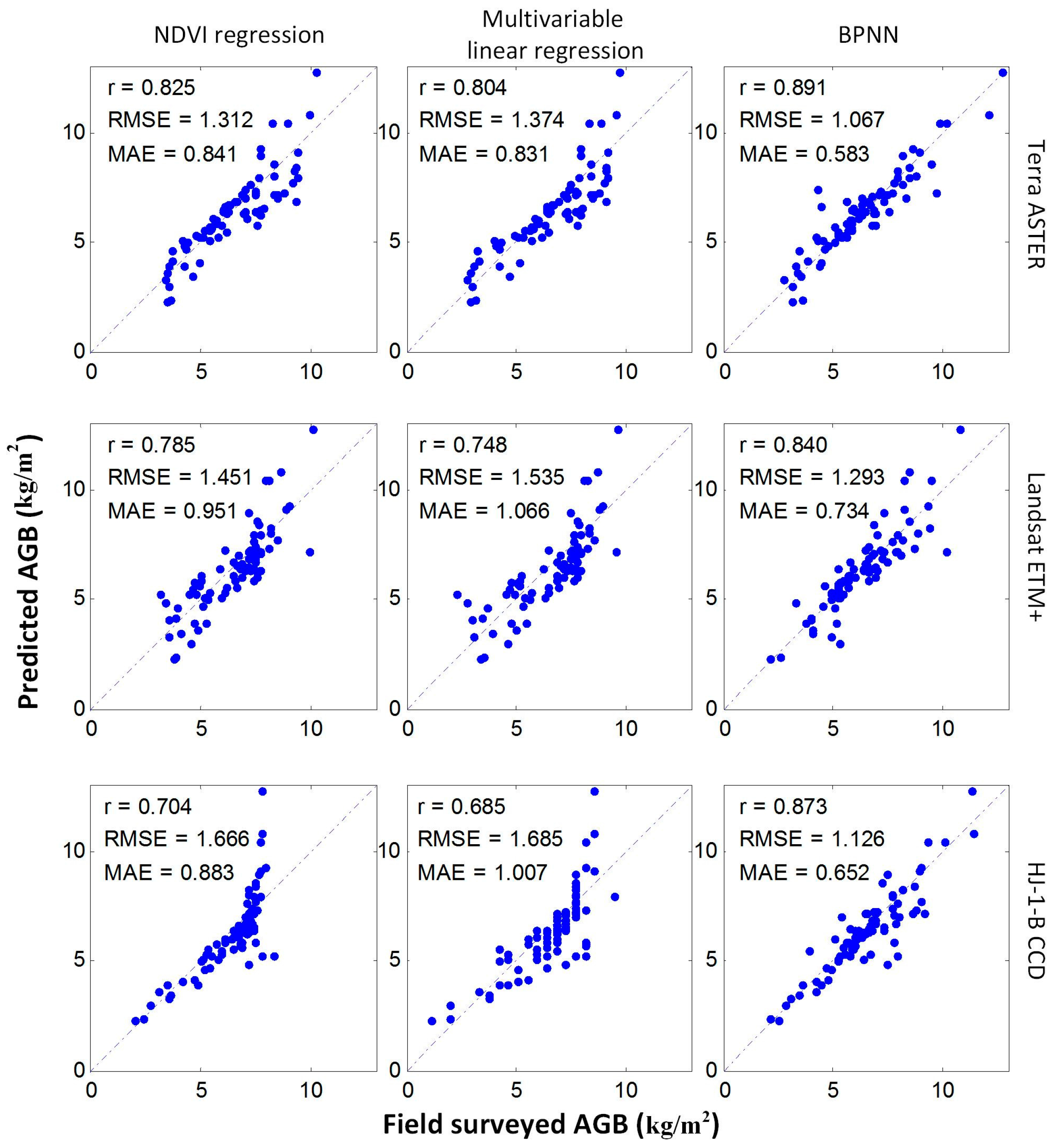
(1)

In the first column, the predicted AGB results were from NDVI data and NDVI regression models. In the second column, the predicted AGB results were from multivariable linear regression models. The regression models for predicting AGB from NDVI were listed in Table 2(a).

(2)

In the first line, the data for predicting AGB were from Terra ASTER images. In the second and the third line, the data were from Landsat ETM+ and HJ-1-B CCD images.

In Figure 7, the independent variables are backscatter coefficients of SAR imagery. In Figure 7a–d, the data for predicting AGB were from Envisat ASAR, where the models are regression models in the first three figures and BPNN model in the last figure. In Figure 7e, the predicted AGB results were from ERS-2 VV data and regression models. These regression models are listed in Table 2(b).

In Figure 8, the independent variables are combinations of SAR and optical images. Figure 8 shows:

(1)

The SAR data used in Figure 8a was from Envisat ASAR, and from ERS-2 in Figure 8b.

(2)

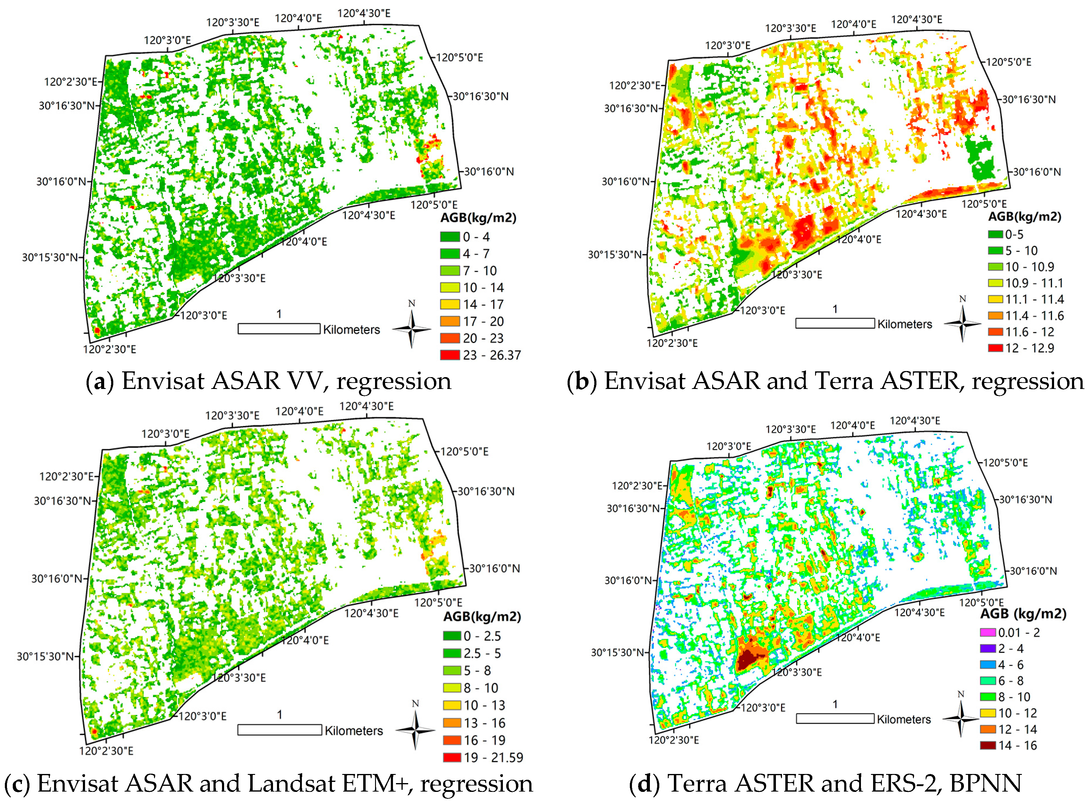
In the first column of Figure 8a,b, the optical data combined with SAR data for predicting AGB was from Terra ASTER. And the optical data was from Landsat ETM+ and HJ-1-B CCD in the second and third column respectively.

(3)

In the first line of Figure 8a,b, the predicted AGB results were from multivariable linear regression models. The models are listed in Table 2(c,d). One variable was introduced and the other variables were excluded in some models.

(4)

In the second line, the predicted AGB results were predicted from BPNN models.

5. Discussion

5.1. Comparison of Models by Sensor Type

Regarding the AGB models generated from optical data, Table 2(a), Terra ASTER models and Landsat ETM+ models are similar. The functional form of both NDVI models and multivariable models introduce only NDVI as independent variable while excluding all other optical data. Hence the models are eventually single variable models. This is reasonable as Terra ASTER has similar green, red and near-infrared bands as Landsat ETM+. Comparing with all lines in Figure 6, Terra ASTER models show better accuracies: they have less RMSE and MAE and greater r. One of the possible reasons is that Terra ASTER has finer spatial resolution in visual and near infrared band (15 m) than Landsat ETM+ and HJ-1-B CCD (30 m). The multivariable regression model from HJ-1-B CCD data excludes all other data and introduces only one variable but it introduces Digital Number (DN) data from the near-infrared band rather than NDVI. When compared with the BPNN models for estimating, AGB from optical data (the third column in Figure 6), the model for Terra ASTER data has maximum r, minimum RMSE and MAE amongst all the BPNN models from optical data.

As for AGB regression models from SAR data, they show better results than the models from optical images: greater R², r and less RMSE, MAE, Table 2(b) and Figure 7. The regression model from ERS-2 SAR data shows a better result in R², r, RMSE and MAE than that from Envisat ASAR. As for Envisat ASAR data, VV polarized data is possibly more related to AGB than HH polarized data, as the R² and r are greater and RMSE and MAE is less. The multivariate linear regression model from Envisat ASAR VV and HH data is acceptable as the VIF equals 4.868 (less than 5, though greater than 3). However, Envisat ASAR has improved instruments, based on the instrument of ERS-1 and ERS-2, so that it has better performance. The model accuracy implies some potential limitation such as in field inventory, or in the geocorrection on remote sensing images.

Regarding BPNN models, the model from Envisat ASAR data shows better results than that from optical imagery: (1) r is 0.961 compared to 0.891, 0.840 and 0.873 from Terra ASTER, Landsat ETM+ and HJ-1-B CCD image; (2) RMSE of models from these optical images are 158%, 192%, 167% of RMSE result from Envisat ASAR data; (3) MAE of models from these optical images are 123%, 155%, 137% of MAE result from Envisat ASAR data. The possible reason is that the optical sensor receives the surface reflectance rather than the volumetric scattering of vegetation, thus the estimates of AGB are limited by a loss of sensitivity with increasing biomass, commonly known as “saturation” [8]; while C-band SAR backscatter provides vegetation structure information, including the scattering components from the ground surface, the canopy as well as the interaction between these components. Together, these components account for volumetric scattering that is related to AGB [58,59].

It is discussed in Section 4.1 that both optical and SAR images play roles in retrieval of VCLA. We tested generating regression models for estimating AGB combining optical and SAR images. The results, Table 2(c,d), show that the models from ERS-2 combining Terra ASTER or Landsat ETM+ images are better than the models from Envisat ASAR combining these two types of optical images. For example, R² are respectively 0.870, 0.841, compared to 0.806 and 0.807. While comparing the ERS-2 and HJ-1-B CCD combined model with Envisat ASAR and HJ-1-B CCD combined model, they show similar quality. ERS-2 and Terra ASTER combination yields a model with the greatest R² (0.870) amongst all the linear regression models. It is slightly lower than Envisat ASAR or ERS-2 ${\mathsf{\sigma }}_{VV}^0$ models (0.874 and 0.871). The model has least RMSE (0.395 kg/m²) and MAE (0.256 kg/m²) among all the regression models (Figure 7 and Figure 8). Additionally, the BPNN models from a combination of SAR and optical image is generally better in r, RMSE and MAE, except the BPNN model from the Envisat ASAR VV/HH image. Comparing Table 2(a) and Figure 6 with other tables and figures, the models from optical sensors show lower accuracies than the models from the SAR combinations in this study.

5.2. Comparison of Modeling Methods

The modeling method used in this analysis can be classified in three categories as: (1) single variable regression model; (2) multivariable regression model; (3) BPNN model.

We implemented curve estimation to generate single variable models. The chosen models have the maximum R², as listed in Table 2(a,b). It is noticed that all single variable models are exponential models. Comparing all the single variable and multivariable regression models, the selected exponential models better described the relation between AGB and remote sensing data. For example, the R² value of Terra ASTER NDVI, Envisat ASAR VV polarization and ERS-2 VV polarization models are respectively 0.775, 0.874 and 0.871, compared to 0.642, 0.796 and 0.804 of the linear models.

We also implemented linear regression for multivariable models. More than one variable was inputted to SPSS 20 for generating linear models. In some cases, all the other independent data were excluded in a stepwise regression. Meanwhile, some models were automatically or manually omitted as VIF is greater than 5, even greater than 1000 in some omitted models. A possible explanation is that VIs appear to be related with red and near-infrared reflectance. This leads to a single linear variable model. For example, we input spectral reflectance and VIs of Terra ASTER or Landsat ETM+ and generated a single variable linear model, Table 2(a).

Some of the multivariable linear regression models have lower R² than the single independent models mentioned above. For example, R² of Envisat ASAR ${\mathsf{\sigma }}_{VV}^0$ and ${\mathsf{\sigma }}_{HH}^0$ nonlinear models are respectively 0.874 and 0.861, comparing with 0.823 of Envisat ASAR ${\mathsf{\sigma }}_{VV}^0$, ${\mathsf{\sigma }}_{HH}^0$ multivariable regression model and 0.806 or 0.807 of multivariable regression model from Envisat ASAR with Terra ASTER or with Landsat ETM+. Consulting the curve estimation models in Table 2(a,b), spectral data and VIs are possibly in nonlinear relation with AGB. In future analysis, we will implement another method to generate models with possibly greater accuracies: (1) each variable is analysed using the curve estimation method, so as to determine the functional form between AGB and these variables (e.g., exponential function, logarithmic function and power function); (2) transform each variable according to the curve estimation results, so that the transformed variables are more possibly in linear relation with AGB; (3) input the transformed variables to build multivariable linear regression models for AGB estimation.

Another method implemented in this study was BPNN modeling. We chose 60% of the field sampled data for training. Comparing the third line with the first and second line in Figure 6, the BPNN models show better results of r, RMSE and MAE. For example in the first line, r is 0.891 for BPNN models from Terra ASTER data, greater than 0.825 for NDVI regression model and 0.804 for multivariable linear regression models; actually a linear regression model with only one variable, as shown in the second line in Table 2(a). The same conclusion is drawn comparing Figure 7d with Figure 7a,c,e and comparing the second line with the first line in Figure 8. The BPNN model from the combination of Terra ASTER and ERS-2 SAR image has the least RMSE (0.396 kg/m²), the least MAE (0.256 kg/m²) and the greatest r (0.974). It should be addressed again that there is less field sampling data used in generating ERS-2 SAR models because the study area is quite close to the western boundary of the ERS-2 SAR image used in this analysis, so that the ERS-2 SAR image does not cover some of the sampled areas.

5.3. AGB Distribution

We selected some models for predicting AGB. The selected models are the first model in Table 2(a), the first model in Table 2(b), the first and second model in Table 2(c), also the BPNN model from Terra ASTER and ERS-2 SAR image. These models have lower RMSE, MAE and higher value in each kind of sensor type of combination. The remote sensing data used for prediction are listed in Table 1. As is discussed at the end of Section 5.1, models from optical sensors show lower accuracies in this study. In the predicted AGB map using the model in the first line of Table 2(a), the AGB was too high in some areas (greater than 50 kg/m²). So we excluded this map and show other AGB maps in Figure 9. Figure 9a–d show distribution of vegetation and AGB in the study area. But there were some differences between these maps. High AGB locations varied as modeling data and method. This implies some limitation of our modeling results.

According to the classification map (Figure 5), many fragmented water areas and vegetation regions lie in the western part of the Xixi National Wetland Park. These maps show that the western part of this wetland is better protected than the eastern part. The eastern part is closer to the central city of Hangzhou. There is a patch with few AGB around 30°16′30″N, 120°04′05″E and another patch around 30°16′00″N, 120°04′35″E. A spot at high AGB level lies in the southwest corner of the study area. Figure 9a,c,d show that some small patches at high AGB level can be found in the eastern part (near 30°16′10″N, 120°05′00″E). Figure 9b,d show that some small patches at high AGB level can be found in the western part (near 30°15′30″N, 120°03′10″E). Besides, a continuous area at comparatively high AGB level lies in the northwest corner.

Total AGB also varies between maps. In Figure 9a–d, the total AGB were respectively 186,321 kg/m², 266,513 kg/m², 168,497 kg/m² and 209,580 kg/m². In Figure 9b, most of the pixel values with AGB were greater than 5 kg/m². That is possibly greater than the actual AGB. We therefore cautiously estimate that the total AGB in the study area is between 165,000 and 210,000 kg/m².

6. Conclusions

We developed a set of models for predicting AGB in Xixi National Wetland Park using remote sensing images. Optical images, a series of derived VIs and SAR images are used in the estimation process. VCLA is retrieved through a supervised classification before modeling. During the modeling process, all the AGB information and remote sensing data were from VCLA. Therefore land cover should be classified before using these predicting models. We tested modeling without classification and returned low accuracy models: R² are less than 0.4. The accuracy is significantly improved with a classification process.

The modeling methods consist of (1) curve estimation; (2) linear regression for multivariable model; (3) BPNN modeling. According to the NDVI models and multivariable models, Terra ASTER models and Landsat ETM+ models are similar in the functional form. As for SAR model, VV polarized data is slightly more related to AGB than the HH polarized data. The models from ERS-2 combining Terra ASTER, or combining Landsat ETM+ image show better accuracies than the models from Envisat ASAR combining these 2 types of optical image. As for curve estimation, all single variable models derived are exponential models. In the BPNN modeling, SAR models generally showed better accuracy than optical models. Among all the models, the BPNN model from Terra ASTER combining ERS-2 data showed the greatest accuracy. Some multivariate models are omitted due to the multicollinearity problem. We cautiously estimate that the total AGB in this area was between 165,000 and 210,000 kg/m².

Promising results can be derived by integrating SAR and optical imagery, although there are still four potential limitations in this study.

(1)

There exists some potential disagreement between remote sensing data and field inventory. Field sampling was carried out in March and April and early May in 2009. All the images were not acquired in this period, but mainly in March or April in the year 2009. The Envisat ASAR image was acquired in August when the vegetation was in another growing season.

(2)

One of the potential reasons that decrease accuracy is that all optical images were resampled to 12.5 m in resolution but the original resolution was 15 m for Terra ASTER, 30 m for Landsat ETM+ and HJ-1-B CCD.

(3)

As the curve estimation yielded nonlinear models, Table 2, spectral data and VIs are possibly in nonlinear relation with AGB. This is also addressed in Section 5.2. The accuracy would be improved in multivariable nonlinear regression models.

(4)

Differences exist between predicted AGB maps derived from different modeling method and input data. The results should be compared with analysis from other studies, so as to choose better models. Currently there are no AGB studies in this area.

ERS-2 was retired on 5 September 2011 and Envisat mission ended on 8 April 2012. Fortunately HJ-1-C was launched on November 2012. Future analysis will focus on the combination of HJ-1 optical imagery (on Satellite A and B) and SAR (on Satellite C) imagery for seasonal analysis of AGB in our study area.

References

- Kokaly, R.F.; Despain, D.G.; Clark, R.N.; Livo, K.E. Mapping vegetation in Yellowstone national park using spectral feature analysis of aviris data. Remote Sens. Environ. 2003, 84, 437–456. [Google Scholar] [CrossRef]
- Bustamante, J.; Pacios, F.; Díaz-Delgado, R.; Aragonés, D. Predictive models of turbidity and water depth in the Doñana marshes using Landsat TM and ETM+ images. J. Environ. Manag. 2009, 90, 2219–2225. [Google Scholar] [CrossRef] [PubMed]
- Díaz-Delgado, R.; Aragonés, D.; Ameztoy, I.; Bustamante, J. Monitoring marsh dynamics through remote sensing. In Conservation Monitoring in Freshwater Habitats; Springer: Dordrecht, The Netherlands, 2010; pp. 375–386. [Google Scholar]
- Dąbrowska-Zielińska, K.; Budzyńska, M.; Kowalik, W.; Małek, I.; Gatkowska, M.; Bartold, M. Biophysical parameters assessed from microwave and optical data. AEU Int. J. Electron. Commun. 2012, 58, 99–104. [Google Scholar] [CrossRef]
- Zoffoli, M.L.; Kandus, P.; Madanes, N.; Calvo, D.H. Seasonal and interannual analysis of wetlands in South America using NOAA-AVHRR NDVI time series: The case of the Parana Delta Region. Landsc. Ecol. 2008, 23, 833–848. [Google Scholar] [CrossRef]
- Goetz, S.; Dubayah, R. Advances in remote sensing technology and implications for measuring and monitoring forest carbon stocks and change. Carbon Manag. 2011, 2, 231–244. [Google Scholar] [CrossRef]
- Liao, J.; Dong, L.; Shen, G. Neural network algorithm and backscattering model for biomass estimation of wetland vegetation in Poyang Lake area using Envisat ASAR data. In Proceedings of the International Geoscience and Remote Sensing Symposium (IGARSS), Cape Town, South Africa, 13–17 July 2009.
- Zolkos, S.G.; Goetz, S.J.; Dubayah, R. A meta-analysis of terrestrial aboveground biomass estimation using LiDAR remote sensing. Remote Sens. Environ. 2013, 128, 289–298. [Google Scholar] [CrossRef]
- Li, X. Study of urban wetland park development in Chongqing. In Informatics and Management Science VI; Springer: London, UK, 2013; pp. 217–225. [Google Scholar]
- Haase, D.; Larondelle, N.; Andersson, E.; Artmann, M.; Borgström, S.; Breuste, J.; Gomez-Baggethun, E.; Gren, Å.; Hamstead, Z.; Hansen, R.; et al. A quantitative review of urban ecosystem service assessments: Concepts, models, and implementation. Ambio 2014, 43, 413–433. [Google Scholar] [CrossRef] [PubMed]
- Schetke, S.; Haase, D.; Breuste, J.H. Green space functionality under conditions of uneven urban land use development. J. Land Use Sci. 2010, 5, 143–158. [Google Scholar] [CrossRef]
- Kapil, N.; Bhattacharyya, K.G. Spatial, temporal and depth profiles of trace metals in an urban wetland system: A case study with respect to the Deepor Beel, Ramsar site 1207. India. Environ. Pollut. 2012, 2, 51–72. [Google Scholar] [CrossRef]
- Zhang, D.; Jinadasa, K.B.S.N.; Gersberg, R.M.; Liu, Y.; Ng, W.J.; Tan, S.K. Application of constructed wetlands for wastewater treatment in developing countries—A review of recent developments (2000–2013). J. Environ. Manag. 2014, 141, 116–131. [Google Scholar] [CrossRef] [PubMed]
- Lang, M.; Bourgeau-Chavez, L.L.; Tiner, R.W.; Klemas, V.V. Advances in remotely sensed data and techniques for wetland mapping and monitoring. In Remote Sensing of Wetlands: Applications and Advances; Ralph, W.T., Megan, W.L., Victor, V.K., Eds.; CRC Press: Boca Raton, FL, USA, 2015; Chapter 5; pp. 79–118. [Google Scholar]
- Adam, E.; Mutanga, O.; Rugege, D. Multispectral and hyperspectral remote sensing for identification and mapping of wetland vegetation: A review. Wetl. Ecol. Manag. 2010, 18, 281–296. [Google Scholar] [CrossRef]
- Moreau, S.; Bosseno, R.; Gu, X.F.; Baret, F. Assessing the biomass dynamics of Andean bofedal and totora high-protein wetland grasses from NOAA/AVHRR. Remote Sens. Environ. 2003, 85, 516–529. [Google Scholar] [CrossRef]
- Zhao, B.; Yan, Y.; Guo, H.; He, M.; Gu, Y.; Li, B. Monitoring rapid vegetation succession in estuarine wetland using time series MODIS-based indicators: An application in the Yangtze River Delta area. Ecol. Indic. 2009, 9, 346–356. [Google Scholar] [CrossRef]
- Xie, P.; He, B.; Xing, M. Estimation above-ground biomass of wetland bulrush in Qaidam Basin, China, combining regression model with vegetation index. In Proceedings of the 2011 19th International Conference on Geoinformatics, Shanghai, China, 24–26 June 2011.
- Chen, W.; Zorn, P.; Chen, Z.; Latifovic, R.; Zhang, Y.; Li, J.; Quirouette, J.; Olthof, I.; Fraser, R.; Mclennan, D.; et al. Propagation of errors associated with scaling foliage biomass from field measurements to remote sensing data over a northern Canadian national park. Remote Sens. Environ. 2013, 130, 205–218. [Google Scholar] [CrossRef]
- Dillabaugh, K.A.; King, D.J. Riparian marshland composition and biomass mapping using IKONOS imagery. Can. J. Remote Sens. 2008, 34, 143–158. [Google Scholar] [CrossRef]
- Ghioca-Robrecht, D.M.; Johnston, C.A.; Tulbure, M.G. Assessing the use of multiseason QuickBird imagery for mapping invasive species in a Lake Erie coastal Marsh. Wetlands 2008, 28, 1028–1039. [Google Scholar] [CrossRef]
- Davranche, A.; Lefebvre, G.; Poulin, B. Wetland monitoring using classification trees and SPOT-5 seasonal time series. Remote Sens. Environ. 2010, 114, 552–562. [Google Scholar] [CrossRef]
- Moreau, S.; Le Toan, T. Biomass quantification of Andean wetland forages using ERS satellite SAR data for optimizing livestock management. Remote Sens. Environ. 2003, 84, 477–492. [Google Scholar] [CrossRef]
- Grings, F.; Salvia, M.; Karszenbaum, H.; Ferrazzoli, P.; Perna, P.; Barber, M.; Berlles, J.J. Statistical information of ASAR observations over wetland areas: An interaction model interpretation. ISPRS J. Photogramm. Remote Sens. 2010, 65, 77–85. [Google Scholar] [CrossRef]
- Chen, J.; Lin, H.; Huang, C.; Fang, C. The relationship between the leaf area index (LAI) of rice and the C-band SAR vertical/horizontal (VV/HH) polarization ratio. Int. J. Remote Sens. 2009, 30, 2149–2154. [Google Scholar]
- Pandey, U.; Kushwaha, S.P.S.; Kachhwaha, T.S.; Kunwar, P.; Dadhwal, V.K. Potential of Envisat ASAR data for woody biomass assessment. Trop. Ecol. 2010, 51, 117–124. [Google Scholar]
- Dabrowska-Zielinska, K.; Gruszczynska, M.; Lewinski, S.; Hoscilo, A.; Bojanowski, J. Application of remote and in situ information to the management of wetlands in Poland. J. Environ. Manag. 2009, 90, 2261–2269. [Google Scholar] [CrossRef] [PubMed]
- Sun, Y.; Gong, H.; Li, X.; Pu, R.; Li, S. Extracting eco-hydrological information of inland wetland from L-band Synthetic Aperture Radar image in Honghe National Nature Reserve, Northeast China. Chin. Geogr. Sci. 2011, 21, 241–248. [Google Scholar] [CrossRef]
- Gama, F.F.; Dos Santos, J.R.; Mura, J.C. Eucalyptus biomass and volume estimation using interferometric and polarimetric SAR data. Remote Sens. 2010, 2, 939–956. [Google Scholar] [CrossRef]
- Santos, J.R.; Lacruz, M.S.P.; Araujo, L.S.; Keil, M. Savanna and tropical rainforest biomass estimation and spatialization using JERS-1 data. Int. J. Remote Sens. 2002, 23, 1217–1229. [Google Scholar] [CrossRef]
- Collins, J.N.; Hutley, L.B.; Williams, R.J.; Boggs, G.; Bell, D.; Bartolo, R. Estimating landscape-scale vegetation carbon stocks using airborne multi-frequency polarimetric synthetic aperture radar (SAR) in the savannahs of north australia. Int. J. Remote Sens. 2009, 30, 1141–1159. [Google Scholar] [CrossRef]
- Huang, W.; Sun, G.; Ni, W.; Zhang, Z.; Dubayah, R. Sensitivity of multi-source SAR backscatter to changes in forest aboveground biomass. Remote Sens. 2015, 7, 9587–9609. [Google Scholar] [CrossRef]
- Cutler, M.E.J.; Boyd, D.S.; Foody, G.M.; Vetrivel, A. Estimating tropical forest biomass with a combination of SAR image texture and Landsat TM data: An assessment of predictions between regions. ISPRS J. Photogramm. Remote Sens. 2012, 70, 66–77. [Google Scholar] [CrossRef]
- Li, X.; Yeh, A.G.O.; Wang, S.; Liu, K.; Liu, X. Estimating mangrove wetland biomass using radar remote sensing. J. Remote Sens. 2006, 10, 387–396. [Google Scholar]
- Anderson, J.E. Spectral Signatures of Wetlands Plants (350–900 nm); Army Topographic Engineering Center Fort Belvoir VA: Alexandria, VA, USA, 1995. [Google Scholar]
- Shen, G.; Liao, J.; Guo, H.; Liu, J.; Zhang, L.; Chen, J. Wetland vegetation biomass inversion using polarimetric RADARSAT-2 data. In Proceedings of the 2012 IEEE International Geoscience and Remote Sensing Symposium (IGARSS), Munich, Germany, 22–27 July 2012.
- Sexton, R.S.; Dorsey, R.E.; Johnson, J.D. Optimization of neural networks: A comparative analysis of the genetic algorithm and simulated annealing. Eur. J. Oper. Res. 1999, 114, 589–601. [Google Scholar] [CrossRef]
- Baştürk, A.; Günay, E. Efficient edge detection in digital images using a cellular neural network optimized by differential evolution algorithm. Expert Syst. Appl. 2009, 36, 2645–2650. [Google Scholar] [CrossRef]
- Shen, Q.; Liu, K.; Li, S.; Zhang, J.; Jiang, Y.; Ge, Y.; Chang, J. Relationships of plant composition, water level and solar radiation in Xixi Wetland, Hangzhou, China. J. Plant Ecol. 2008, 32, 114–122. [Google Scholar]
- Zhou, H.; Jiang, H.; Zhou, G.; Song, X.; Yu, S.; Chang, J.; Liu, S.; Jiang, Z.; Jiang, B. Monitoring the change of urban wetland using high spatial resolution remote sensing data. Int. J. Remote Sens. 2010, 31, 1717–1731. [Google Scholar] [CrossRef]
- Bonham, C.D. Measurements for Terrestrial Vegetation; John Wiley & Sons: Hoboken, NJ, USA, 2013. [Google Scholar]
- Parresol, B.R. Assessing tree and stand biomass: A review with examples and critical comparisons. For. Sci. 1999, 45, 573–593. [Google Scholar]
- Brown, S. Measuring carbon in forests: Current status and future challenges. Environ. Pollut. 2002, 116, 363–372. [Google Scholar] [CrossRef]
- Wang, Q.; Wu, C.; Li, Q.; Li, J. Chinese HJ-1A/B satellites and data characteristics. Sci. China Ser. D 2010, 53, 51–57. [Google Scholar] [CrossRef]
- Tucker, C.J. Red and photographic infrared linear combinations for monitoring vegetation. Remote Sens. Environ. 1979, 8, 127–150. [Google Scholar] [CrossRef]
- Bannari, A.; Morin, D.; Bonn, F.; Huete, A.R. A review of vegetation indices. Remote Sens. Rev. 1995, 13, 95–120. [Google Scholar] [CrossRef]
- Purevdorj, T.S.; Tateishi, R.; Ishiyama, T.; Honda, Y. Relationships between percent vegetation cover and vegetation indices. Int. J. Remote Sens. 1998, 19, 3519–3535. [Google Scholar] [CrossRef]
- Huang, C.; Shao, Y.; Liu, J.; Chen, J. Temporal analysis of urban forest in Beijing using Landsat imagery. J. Appl. Remote Sens. 2007, 1, 1–12. [Google Scholar] [CrossRef]
- Glenn, E.P.; Huete, A.R.; Nagler, P.L.; Nelson, S.G. Relationship between remotely-sensed vegetation indices, canopy attributes and plant physiological processes: What vegetation indices can and cannot tell us about the landscape. Sensors 2008, 8, 2136–2160. [Google Scholar] [CrossRef]
- Pinty, B.; Verstraete, M.M. GEMI: A non-linear index to monitor global vegetation from satellites. Vegetatio 1992, 101, 15–20. [Google Scholar] [CrossRef]
- Wu, J.; Gao, W.; Tueller, P.T. Effects of changing spatial scale on the results of statistical analysis with landscape data: A case study. Geogr. Inf. Sci. 1997, 3, 30–41. [Google Scholar] [CrossRef]
- Roujean, J.L.; Breon, F.M. Estimating PAR absorbed by vegetation from bidirectional reflectance measurements. Remote Sens. Environ. 1995, 51, 375–384. [Google Scholar] [CrossRef]
- Rundquist, D.; Gitelson, A.; Lawson, M.; Keydan, G.; Leavitt, B.; Perk, R.; Keck, J.; Mishra, D.R.; Narumalani, S. Proximal sensing of coral features: Spectral characterization of Siderastrea siderea. GISci. Remote Sens. 2009, 46, 139–160. [Google Scholar] [CrossRef]
- Gu, Z.; Shi, X.; Li, L.; Yu, D.; Liu, L.; Zhang, W. Using multiple radiometric correction images to estimate leaf area index. Int. J. Remote Sens. 2011, 32, 9441–9454. [Google Scholar] [CrossRef]
- Deng, C.; Wu, C. Examining the impacts of urban biophysical compositions on surface urban heat island: A spectral unmixing and thermal mixing approach. Remote Sens. Environ. 2013, 131, 262–274. [Google Scholar] [CrossRef]
- Chen, J.; Zeng, Z.; Jiang, P.; Tang, H. Deformation prediction of landslide based on functional network. Neurocomputing 2015, 149, 151–157. [Google Scholar] [CrossRef]
- Chen, T.; Chang, Q.; Clevers, J.G.P.W.; Kooistra, L. Rapid identification of soil cadmium pollution risk at regional scale based on visible and near-infrared spectroscopy. Environ. Pollut. 2015, 206, 217–226. [Google Scholar] [CrossRef] [PubMed]
- Treuhaft, R.N.; Siqueira, P.R. The calculated performance of forest structure and biomass estimates from interferometric radar. Wave Random Media 2004, 14, S345–S358. [Google Scholar] [CrossRef]
- Montesano, P.M.; Cook, B.D.; Sun, G.; Simard, M.; Nelson, R.F.; Ranson, K.J.; Zhang, Z.; Luthcke, S. Achieving accuracy requirements for forest biomass mapping: A spaceborne data fusion method for estimating forest biomass and LiDAR sampling error. Remote Sens. Environ. 2013, 130, 153–170. [Google Scholar] [CrossRef]