Regional Estimation of Remotely Sensed Evapotranspiration Using the Surface Energy Balance-Advection (SEB-A) Method

Abstract

Evapotranspiration (ET) is an essential part of the hydrological cycle and accurately estimating it plays a crucial role in water resource management. Surface energy balance (SEB) models are widely used to estimate regional ET with remote sensing. The presence of horizontal advection, however, perturbs the surface energy balance system and contributes to the uncertainty of energy influxes. Thus, it is vital to consider horizontal advection when applying SEB models to estimate ET. This study proposes an innovative and simplified approach, the surface energy balance-advection (SEB-A) method, which is based on the energy balance theory and also takes into account the horizontal advection to determine ET by remote sensing. The SEB-A method considers that the actual ET consists of two parts: the local ET that is regulated by the energy balance system and the exotic ET that arises from horizontal advection. To evaluate the SEB-A method, it was applied to the middle region of the Heihe River in China. Instantaneous ET for three days were acquired and assessed with ET measurements from eddy covariance (EC) systems. The results demonstrated that the ET estimates had a high accuracy, with a correlation coefficient (R²) of 0.713, a mean average error (MAE) of 39.3 W/m² and a root mean square error (RMSE) of 54.6 W/m² between the estimates and corresponding measurements. Percent error was calculated to more rigorously assess the accuracy of these estimates, and it ranged from 0% to 35%, with over 80% of the locations within a 20% error. To better understand the SEB-A method, the relationship between the ET estimates and land use types was analyzed, and the results indicated that the ET estimates had spatial distributions that correlated with vegetation patterns and could well demonstrate the ET differences caused by different land use types. The sensitivity analysis suggested that the SEB-A method requested accurate estimation of the available energy, $R_n-G$, but was less constrained with the difference between ground and air temperature, $T_0-T_{a–loc}$.

1. Introduction

Evapotranspiration (ET), which is a combined process of evaporation and transpiration, is crucial to the hydrological cycle. It links energy and water exchanges among the hydrosphere, atmosphere and biosphere [1,2,3,4,5]. ET is the largest outgoing water flux from the earth’s surface; most precipitation is lost in the form of ET with the percentage varying from region to region globally. In semi-arid regions, the amount of ET is roughly equivalent to the precipitation [6]. Therefore, the accurate quantification of ET is critical to developing a greater understanding of local and global energy and water cycles, global climate change, land atmosphere interactions and ecosystem processes, and beneficial to improving applications in many fields, such as water resources management, drought monitoring and assessment [7], irrigation scheduling, hydrological modeling, weather forecasts and so on [8,9,10,11,12,13]. Ground-based observations of ET have some advantages but the required ground instrumentation is available in a limited number of places and can only obtain localized values of ET, which often cannot satisfy the needs of regional-scale studies. In addition, the employment of instrumentations is always time consuming, labor intensive and sometimes subject to instrument failure [9].

Recent developments in remote sensing have made it possible to acquire crucial variables for characterizing land surface interactions. Over the last two decades, the requirement of quantifying ET at a regional scale, together with the recent advances in satellite remote sensing technology, has led to many studies on mapping large-scale ET [9,11,14,15]. The surface energy balance algorithm based on the energy balance equation (SEB; Equation (1)), is one of the most widely used approaches for obtaining regional estimates of remotely sensed ET at multiple temporal and spatial scales [9]. Energy and mass are exchanged between the land surface and the atmosphere [16,17]. When the heat fluxes that are transported by horizontal advection and consumed by photosynthetic vegetation are not considered, the one-dimensional form of the surface energy balance equation on an instantaneous time scale can be expressed as:

$$R_n=G+H+LE$$

(1)

where $R_n$ (W/m²) is the net surface radiation, $G$ (W/m²) is the soil heat flux, $H$ (W/m²) is the sensible heat flux, and $LE$ (W/m²) is the latent heat flux. In Equation (1), sensible heat flux can be calculated using the remotely sensed surface temperature, air temperature and a series of conductance formulas; estimates of $R_n$ and G are available using remote sensing or ground data, and hence, the latent heat flux is taken as a residual term of Equation (1) [16,17].

Based on how the sinks or sources of heat fluxes are parameterized between the earth’s surface and the atmosphere, SEB models can be divided into two categories: the single-source models and two-source models, or multi-source models [18]. Single-source SEB models consider vegetation and soil to be a single unit and often utilize land surface temperature (LST) and empirical resistance corrections to derive the latent heat flux [19]. Since they are highly dependent on empirical corrections, single-source SEB models are inappropriate for application over areas with partial vegetation cover, where significant errors would be found [20,21,22]. To overcome the limitations associated with single-source SEB models in partially vegetated areas [22], it is necessary to apply a two-source SEB model that separately simulates the heat and water exchange and the interactions between soil and atmosphere and between vegetation and atmosphere. Thus, in two-source SEB models, the component H is partitioned between the soil and vegetation, and the component LE is treated as the sum of evaporation from the soil surface and transpiration from vegetation.

From the aforementioned review of SEB models, we know that both single-source and two-source models are based on the energy balance equation (Equation (1)) that is founded on the premise of ignoring the energy transported by horizontal advection and consumed by photosynthesis [16,17]. Nevertheless, the presence of horizontal advection always characterizes exchanges in the near surface layer and contributes to the uncertainty of energy influxes [23,24]. Neglecting systematic sampling errors, systematic instrument bias, low and high frequency loss of turbulent fluxes and energy sinks, horizontal advection of heat and water vapor is regarded as the primary reason for the non-closure of the surface energy balance [25,26,27]. To a certain region, uncertainties from horizontal advection on the surface energy balance have two aspects. One is the horizontal advection itself, which develops on heterogeneous surfaces and exerts profound influence on the energy balance equation. This has been reported in many previous studies [28,29]. Therefore, horizontal advection should be discussed as one reason for energy imbalances and regarded as a necessary item to add to the energy balance equation. The other uncertainty refers to the ground-based meteorological variables of air temperature, humidity and other auxiliary surface measurements inputted to the energy balance equation. These meteorological variables are actually measured and thus characterize the practical circumstance rather than describe the environment under the condition of energy balance closure, which means that the actually observed meteorological variables have already contained effects from the horizontal advection and would affect the energy balance equation when they are used as inputs. In conclusion, horizontal advection affects the energy balance equation directly through energy inputs or outputs, whereas ground-based observations impact the energy balance equation indirectly by including the effects of advection.

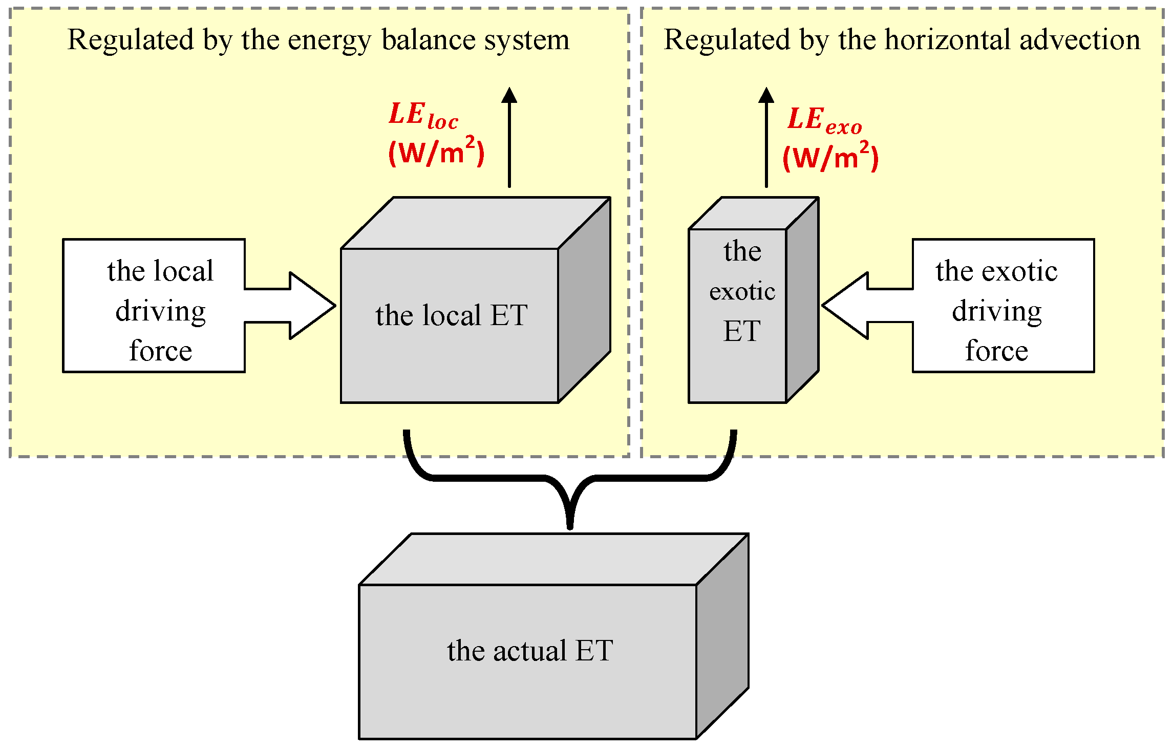
In view of the prevalence of the horizontal advection and its influence on the energy balance system, it is of great necessity to take into account the horizontal advection when applying SEB models to estimate ET. The objective of this paper is to propose an innovative method, the surface energy balance-advection (SEB-A) method, which is based on the energy balance equation and considers the horizontal advection as well to derive ET. The SEB-A method assumes that the energy consumed in the actual ET consists of two parts; one part is provided by the energy balance system and the other part is brought in by the horizontal advection. The former, called local ET, can be obtained by the modified energy balance equation (Equation (3)), and the calculation method of it is similar to previous studies that are on the SEB models; the latter, called exotic ET, can be calculated with the help of ground-based EC observations. Section 2 describes the datasets used to assess the method. Section 3.1 presents a description on the theory of calculating the local ET that is regulated by the energy balance system, and Section 3.2 introduces approaches for deriving the exotic ET that is driven by the horizontal advection. 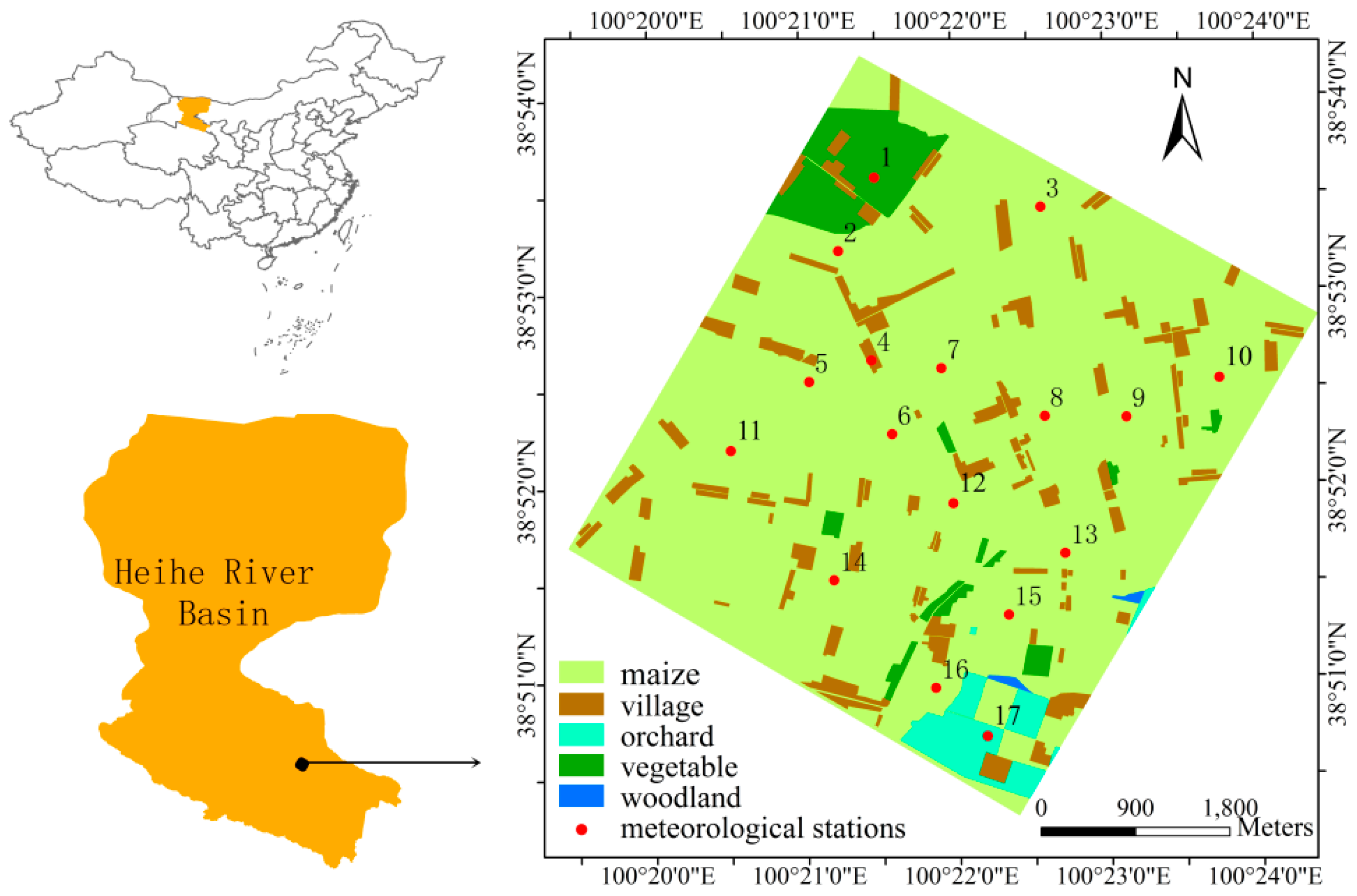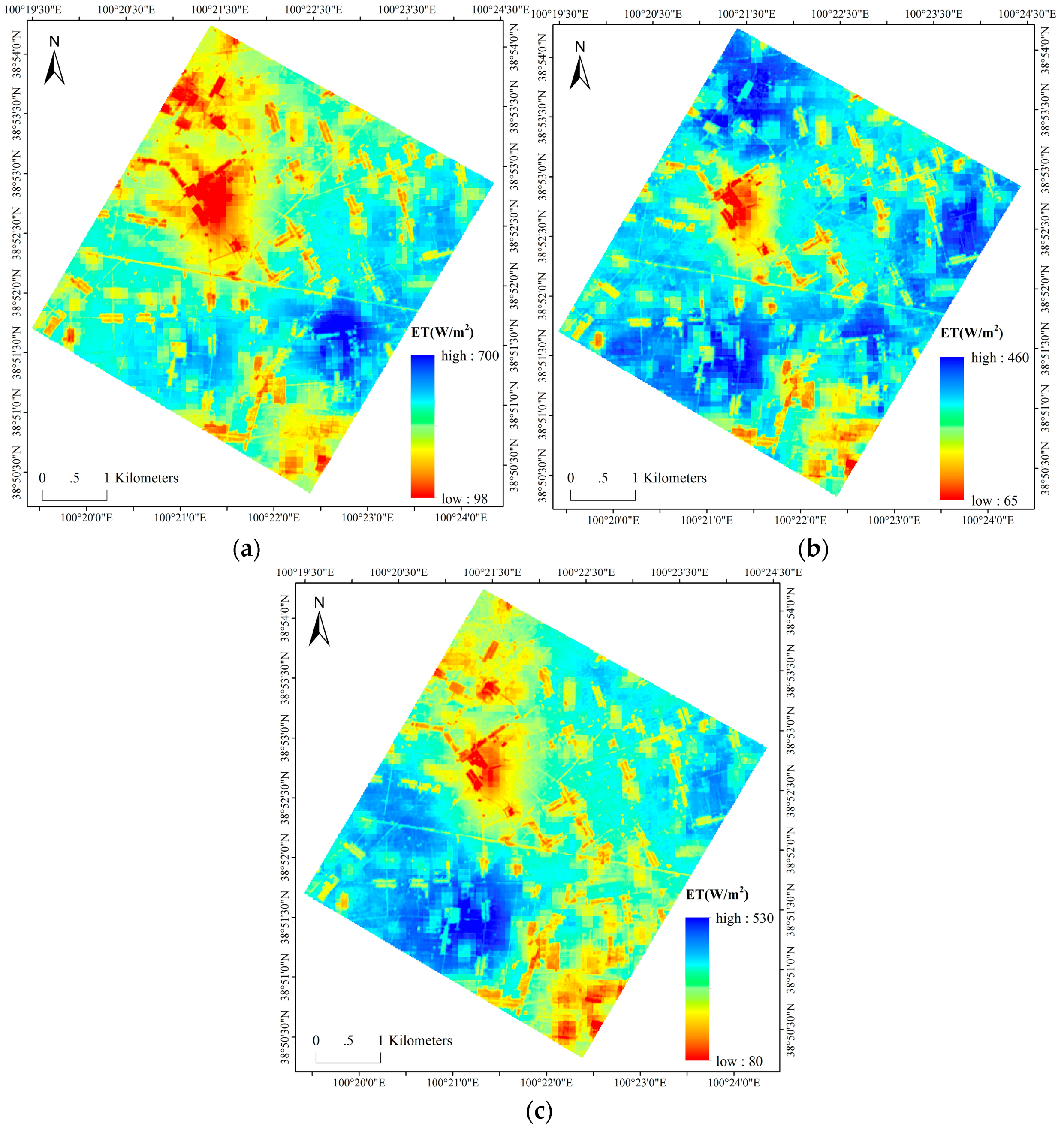Section 4 shows the results of the SEB-A method that was applied on a regional scale by using variables retrieved from ASTER imagery and HJ-1A/B imagery and measured at meteorological and EC stations. Section 5 discusses the advantages and limitations of the SEB-A method. Section 6 concludes the work.

2. Study Area and Datasets

2.1. Study Area

The study area is located in Zhangye, Gansu, China, and it is from 38.83°N to 38.93°N in latitude and from 100.32°E to 100.42°E in longitude, as shown in Figure 1. It belongs to the middle reaches of Heihe River that is the second longest inland river in China. The annual mean air temperature is 7.0 °C. The climate is dry and rainless, with an annual mean precipitation of 124.9 mm and a potential evaporation of 2000 mm. The ground is flat and cultivated with maize, vegetable crops, orchards and woodlands. Some built-up areas (villages) are spread throughout the study area. Every year from May to September, staple crops are grown, including seed corns, vegetables and fruit trees.

To estimate the ET, remote sensing data that include ASTER images and HJ-1A/B images and ground-based observations that include meteorological variables and surface fluxes are required.

2.2. Remote Sensing Data

The ASTER is a sensor that collects multispectral visible, near-infrared and thermal infrared images. It is a special remote sensing tool intended to monitor land surface energy balance, hydrological processes and climate [30]. ASTER images with a high spatial resolution of 15 m in both the visible and near-infrared wave bands (0.52–0.86 µm) were used in this study to estimate the vegetation fraction and the surface emissivity. The LST products, which had a spatial resolution of 90 m, were acquired from the thermal infrared wave band (8.125–11.65 µm) of ASTER images and provided by the Heihe Plan Science Data Center [31,32]. The albedo in the study area was calculated from images acquired from the HJ-1A/B, which is a small satellite constellation that is used for monitoring and forecasting environmental changes and disasters. The HJ-1A/B was launched by China in 2008. Two CCDs (0.45–0.89 µm) with a spatial resolution of 30 m are carried by each satellite.

2.3. Ground Observations

In the study area, there are 17 stations (Figure 1) equipped with Automatic Meteorological Station Systems and EC Systems that are both automatic data acquisition systems. The Automatic Meteorological Station System can acquire meteorological variables, including air temperature, humidity, air pressure, solar radiation, wind speed, wind direction and so on, at sample intervals of 10 min and one minute. The EC System can monitor surface fluxes such as sensible heat flux, latent heat flux and so on, at a sample interval of 30 min.

All data mentioned above were provided by the HiWATER experiment which is an watershed-scale and eco-hydrological experiment designed from an interdisciplinary perspective to address problems that include heterogeneity, scaling, uncertainty and closing of the water cycle at the watershed scale [33]. The experiment was performed in the Heihe River Basin. Users can attain the data by submitting an application to the data center, Cold and Arid Regions Science Data, at Lanzhou (http://westdc.westgis.ac.cn/).

3. Methodology

In this section, the SEB-A method is described in detail. According to previous studies, horizontal advection is the main reason for surface energy imbalances [25,26,27]. As a result, without regard to the internal generating mechanism of ET, the actual ET ($L{E}_{act}$) is directly composed of two parts: the local ET ($L{E}_{loc}$) dominated by the energy balance system, and the exotic ET ($L{E}_{exo}$) given rise to by horizontal advection. This is inspired by the research of Zhang et al. [34].

With no advection or when there is a surface energy balance closure, the actual ET ($L{E}_{act}$) is equal to the local ET ($L{E}_{loc}$) and can be calculated by the energy balance equation. In reality, however, the horizontal advection would perturb the energy balance system and influence the energy balance equation. In this case, the actual ET ($L{E}_{act}$) can be regarded as the sum of the local ET ($L{E}_{loc}$) and the exotic ET ($L{E}_{exo}$). The basic idea can be described as: the local driving force (the energy balance system) produces a local ET, and the exotic driving force (horizontal advection) changes the local ET by adding an exotic ET. The actual ET can be expressed as:

$$L{E}_{act}=L{E}_{loc}+L{E}_{exo}$$

(2)

where $L{E}_{act}$ is the actual ET, $L{E}_{loc}$ is the local ET, and $L{E}_{exo}$ is the exotic ET. Three items are measured in energy units, W/m².

Figure 2 shows the principle of the SEB-A method. Because $L{E}_{act}$ contains both $L{E}_{loc}$ and $L{E}_{exo}$, to estimate $L{E}_{act}$, it is necessary to calculate the two parts: $L{E}_{loc}$ and $L{E}_{exo}$.

3.1. Obtaining the Local ET,$L{E}_{loc}$

The $L{E}_{loc}$ can be determined by using the energy balance equation. Under the condition of energy balance closure, that is to say, there is no horizontal advection, the energy exchange between the land surface and atmosphere can be described by the modified energy balance equation (Equation (3)). Here, we also ignore the energy consumed by photosynthesis.

$$R_n=H_{loc}+L{E}_{loc}+G$$

(3)

where $H_{loc}$ (W/m²) and $L{E}_{loc}$ (W/m²) are the sensible heat flux and the latent heat flux driven by the energy balance system, respectively.

To calculate $L{E}_{loc}$, we need to know the sensible heat flux, $H_{loc}$, as well. It is given as Equation (4):

$$H_{loc}=\frac{\rho C_p}{r_{a–loc}}\left(T_0-T_{a–loc}\right)$$

(4)

where $\rho$ is the air density, $C_p$ (1004 J/(Kg·K)) is the specific heat at constant pressure of air, $r_{a–loc}$ (s/m) is the aerodynamic resistance, $T_0$ (°C) is the aerodynamic temperature that is usually substituted with LST in applications [35,36], and $T_{a–loc}$ (°C) is the surface air temperature when there is no advection. Thus, $L{E}_{loc}$ can be derived as:

$$L{E}_{loc}=R_n-G-\frac{\rho C_p}{r_{a–loc}}\left(\text{LST}-T_{a–loc}\right)$$

(5)

Since there is no horizontal advection, the variables in Equation (5) should be acquired under the condition of energy balance closure. Among these variables, $R_n$, $G$, $\rho C_p$ and LST are thought to remain the same, regardless of whether the energy balance is closed or not on an instantaneous time scale, whereas the other two variables, $r_{a–loc}$ and $T_{a–loc}$, are specific and need to be calculated in the case of energy balance closure.

3.1.1. Calculation of $r_{a–loc}$

The measurement of the special $r_{a–loc}$ was through a laboratory experiment. In the experiment, the observational object was bare soil with a saturated soil water content. Parameters for the calculation including the radiometric soil surface temperature ($T_s$), actual surface vapor pressure ($e_a$) and evaporation ($LE$), were measured with no wind. The formula used for deriving $r_{a–loc}$ is written as:

$$r_{a–loc}=\frac{\rho C_p\left(e_s-e_a\right)}{\gamma LE}-r_s$$

(6)

where $\gamma$ is the psychrometric constant (Pa/K), $r_s$ (s/m) is the surface water vapor resistance and equals zero when the soil is fully saturated, $e_s$ (Pa) is the surface saturated vapor pressure, and $LE$ (g) is the evaporation from the soil and measured by the weighing method.

In the experiment, we set five different initial air conditions with different T_a and RH, and we calculated $r_{a–loc}$ once per hour from 08:00 to 18:00 at the heights of 1 m and 0.5 m, respectively.

Table 1. $r_{a–loc}$ (s/m) measured at a height of 0.5 m.

Time	Ta: 30 RH: 65%	Ta: 25 RH: 55%	Ta: 20 RH: 45%	Ta: 18 RH: 35%	Ta: 15 RH: 30%
8:00	191	140	230	158	132
9:00	179	153	176	167	176
10:00	139	137	165	131	139
11:00	162	146	156	138	153
12:00	146	138	135	131	145
13:00	131	148	166	150	132
14:00	132	139	164	138	151
15:00	133	146	160	152	158
16:00	117	145	149	148	150
17:00	130	141	146	149	141
18:00	129	135	160	156	153
av.	144	143	164	147	148

and

Table 2. $r_{a–loc}$ (s/m) measured at a height of 1 m.

Time	Ta: 30 RH: 65%	Ta: 25 RH: 55%	Ta: 20 RH: 45%	Ta: 18 RH: 35%	Ta: 15 RH: 30%
8:00	182	177	237	166	137
9:00	186	160	172	172	154
10:00	153	134	171	130	146
11:00	164	151	149	135	161
12:00	152	143	130	126	151
13:00	117	148	161	152	138
14:00	133	139	168	140	156
15:00	139	141	162	157	150
16:00	116	149	152	144	161
17:00	149	133	158	142	145
18:00	134	137	164	153	154
av.	148	146	166	147	150

show the calculation results of $r_{a–loc}$ at the heights of 0.5 m and 1 m. In the tables, T_a is the air temperature, RH is the air relative humidity, and av. is the average value of $r_{a–loc}$. The $r_{a–loc}$ varied around 150 s/m, and therefore, a value of $r_{a–loc}$, 150 s/m, was determined and used to compute $L{E}_{loc}$.

3.1.2. Calculation of $T_{a–loc}$

Because $T_{a–loc}$ is specific under the condition of energy balance closure, it can be calculated by the energy balance equation (Equation (3)). Together with the sensible heat flux equation (Equation (4)) and the Bowen ratio, β, equation (Equation (7)), $T_{a–loc}$ can be derived as follows:

$$\beta =\frac{H}{LE}$$

(7)

$$T_{a–loc}=\text{LST}-\frac{\beta \left(R_n-G\right)}{\beta +1}\frac{r_a}{\rho C_p}$$

(8)

In Equation (8), the Bowen ratio, $\beta$, is determined according to an empirical equation presented by Zhang et al. [37]. The equation is written as:

$$\beta =\mathrm{A}\frac{\left(P_{max}-P_{min}\right)-\left(P_i-P_{min}\right)}{\left(P_i-P_{min}\right)}$$

(9)

where $\mathrm{A}$ is an empirical coefficient that equals 0.66, $P$ (W·m⁻²·s^0.5·°C) is the simplified thermal inertia, and $P_{max}$ and $P_{min}$ are, respectively, the maximum and minimum thermal inertia that are determined from the trapezoid space formed by the vegetation index (VI) and LST. The simplified thermal inertia $P$ is defined as:

$$P=\frac{{\overline{R}}_n{\left(t_1-t_1\right)}^{0.5}}{\left(T_{02}-T_{01}\right)}$$

(10)

where ${\overline{R}}_n$ (W/m²) is the average net radiation during $t_1$(s) and $t_2$ (s), $T_{02}$ (°C) is the surface temperature when the satellite is passing, and $T_{01}$ (°C) is the daily minimum surface temperature. $t_2$ and $t_1$ are the occurring times of $T_{02}$ and $T_{01}$, respectively.

3.1.3. Calculation of $R_n$ and $G$

Net radiation, $R_n$, can be derived by Equation (11); soil heat flux, $G$, can be estimated by an empirical equation (Equation (12)) that is used in some previous studies [34].

$$R_n=\left(1-\alpha \right)S_0+R_{ld}-{\epsilon }_s\sigma {T_0}^4$$

(11)

$$G\approx 0.3\left(1-0.9f_v\right)R_n$$

(12)

where $\alpha$ is the surface albedo, $S_0$ (W/m²) is the downward shortwave radiation, $R_{ld}$ (W/m²) is the downward longwave radiation, ${\epsilon }_s$ is the surface emissivity, $\sigma$ (5.67 × 10⁻⁸ W·m⁻²·K⁻⁴) is the Stefan–Boltzmann constant, and $f_v$ is the fraction of vegetated surface.

3.2. Obtaining the Exotic ET, $L{E}_{exo}$

Referring to $L{E}_{exo}$, it requires ground-based observations of latent heat flux to determine its value. For each EC station inputted to the method, we know its local ET, which can be estimated according to Section 3.1 and its actual ET, which is measured by EC stations; then the exotic ET can be determined by Equation (2). However, the attained exotic ET, $L{E}_{exo}$, is ground-based and needs to be extended to a regional scale from a point scale. In the study, we used a spatial interpolation method, the inverse distance weighting (IDW), to interpolate the ground-based $L{E}_{exo}$ to acquire the spatial distribution results. We assume that $L{E}_{exo}$ is affected by the intensity of horizontal advection, which moves to other places through diffusion. Since the IDW interpolates according to the distance between two inputted objectives, it is appropriate to use it to acquire the spatial distribution of $L{E}_{exo}$. The process of interpolation is described as follows.

If the pixel covering the inputted EC station is expressed as Pixel i with $L{E}_{exo\left(i\right)}$, the exotic ET of other pixels (Pixel x, $L{E}_{exo\left(x\right)}$) around Pixel i can be calculated by the IDW. Formulas can be written as:

$$L{E}_{exo\left(x\right)}={\displaystyle \sum }_{\mathrm{i}=1}^{\mathrm{n}}{w}_{\left(i\right)}L{E}_{exo\left(i\right)}$$

(13)

$$w_{\left(i\right)}=\frac{1/{d_i}^k}{{\sum }_{\mathrm{i}=1}^{\mathrm{n}}1/{d_i}^k}$$

(14)

where $L{E}_{exo\left(x\right)}$ (W/m²) is the exotic ET of any pixel to be calculated, $i$ is the number of the inputted EC stations, $w_{\left(i\right)}$ is the weight, $d_i$ (m) is the distance between the Pixel $i$ and Pixel x, and $k$ is the specified power exponent.

4. Results

Three clear sky days, 10 July, 11 August and 27 August 2012, were chosen to conduct the study. The spatially derived ET on three days was arrived at the moment of the ASTER satellite overpass, as shown in Figure 3a–c, respectively. To evaluate the results estimated by the SEB-A method, a result validation, an error analysis, a relationship analysis between ET estimates and land use status and a sensitivity analysis were performed.

4.1. Validation of ET Estimates

The results were validated against measurements from ground-based EC stations. For each of the three days, nine EC stations were used as inputs to the SEB-A method to calculate the exotic ET, and the other eight EC stations were used to verify the estimates. Because three days’ results were tested together, a total of twenty-four points were conducted for the validation. The comparison between estimates obtained by the SEB-A method and measurements from EC stations is shown in Figure 4. It shows that the estimates have an R² of 0.713, a MAE of 39.3 W/m² and an RMSE of 54.6 W/m². Except for three points that have absolute errors higher than 100 W/m² and two points that have absolute errors between 60 W/m² and 70 W/m², the other points have absolute errors lower than 20 W/m². Validation results are similar to previous studies. Kalma made an assessment of some 30 published validations that showed an RMSE value of approximately 50 W/m² and relative errors of 15%–30% [15]. The correlation analysis indicated that the simulated results were quite consistent with the available measurements, illustrating that ET estimates obtained by the SEB-A method were close to the 1:1 line and had high accuracy.

4.2. Error Analysis

To further evaluate the ET estimates, the frequency distribution of the percent errors was analyzed. According to numerical analysis and error analysis theory, the percent error is more scientifically rigorous than the absolute error when making assessments on the accuracy of estimates [38]. The percent error is the absolute error divided by the magnitude of the exact value, and then expressed in terms of per 100. The expression can be written as:

$$\delta =\frac{\Delta }{\mathrm{L}}\times 100\%$$

(15)

where $\delta$ is the percent error, $\Delta$ is the absolute error and $\mathrm{L}$ is the exact value.

Figure 5 displays the frequency distribution of the percent errors on ET estimates, which varies from 0% to 35%. An accuracy of the percent errors within 20% was achieved at more than 80% of study locations, and over 40% of the locations had percent errors lower than 5%.

4.3. Relationship between ET Estimates and Land Use Status

Since spatial distributions of ET estimates were obtained (Figure 3), we can conduct deep analyses by combining the land use types (Figure 1). The land use type within the study area, which was based on the aerial remote sensing data of the Compact Airborne Spectrographic Imager (CASI) and used the Support Vector Machine (SVM) for classification, was also provided by the Heihe Plan Science Data Center [39].

There were five land uses types in the study area, including maize growing, village habitats, vegetable crops, orchards and woodlands. For each land use type, we performed statistical computation and gave an average ET.

Table 3. ET estimates and the exotic ET retrieved by the SEB-A method on five different land use types on 10 July, 11 August and 27 August 2012.

Land Use Type	10 July (W/m2)		11 August (W/m2)		27 August (W/m2)
	$\mathit{L}{\mathit{E}}_{\mathit{a}\mathit{c}\mathit{t}}$	$\mathit{L}{\mathit{E}}_{\mathit{e}\mathit{x}\mathit{o}}$	$\mathit{L}{\mathit{E}}_{\mathit{a}\mathit{c}\mathit{t}}$	$\mathit{L}{\mathit{E}}_{\mathit{e}\mathit{x}\mathit{o}}$	$\mathit{L}{\mathit{E}}_{\mathit{a}\mathit{c}\mathit{t}}$	$\mathit{L}{\mathit{E}}_{\mathit{e}\mathit{x}\mathit{o}}$
maize	528	91	389	36	425	71
vegetable	410	−18	304	23	268	0
orchard	506	66	292	−35	302	−63
woodland	461	53	300	−46	246	27
village	330	−32	177	0	186	22

shows the average ET of each land use type on the three days. Maize had the maximum ET, and the average ETs on the three days were 528 W/m², 389 W/m² and 425 W/m², respectively. Vegetable crops, orchards and woodlands had an average ET between 400 W/m² and 500 W/m² on 10 July and an average ET of approximately 300 W/m² on the other two days. Villages showed the lowest ET, with an average value of 330 W/m² on 10 July and less than 200 W/m² on the other two days. The spatial distribution of ET was intimately linked with vegetation patterns. In general, high ET is in accordance with dense vegetation cover, whereas low ET agrees with sparse vegetation cover. It indicates that the SEB-A method can well demonstrate ET differences caused by land use types. This agrees with previous suggestions that estimating ET at a regional level requires the incorporation of heterogeneous surface conditions [40]. We used the normalized difference vegetation index (NDVI) as an indicator to describe the vegetation characterization and gave phenology of maize, which is the staple crop in the study area. The summarized NDVIs of maize, vegetables, orchards and woodland, and the phenology of maize, are shown in

Table 4. NDVIs of maize, vegetables, orchards and woodlands on 10 July, 11 August and 27 August 2012.

NDVI	10 July	11 August	27 August
maize	0.71	0.71	0.69
vegetable	0.62	0.64	0.60
orchard	0.64	0.65	0.64
woodland	0.66	0.66	0.65

and

Table 5. The phenology of maize in the study area in 2012.

Sowing Date	Seeding Stage	Jointing Stage	Anthesis Stage	Maturity Stage
25 April	10 May	23 June	10 July	10 September

, respectively. In July and August, maize is in its vigorous growth season (Table 5) with frequent irrigation, and hence, the vegetation cover (Table 4) is dense and the ET is high. Because the orchards, vegetation (pepper, celery and cauliflower) and woodlands had sparse vegetation cover compared to the maize during this time, their associated ETs are lower than those of maize. As for villages, they had largely bare and solidified underlying surfaces, and thus their ETs were the lowest. These results are consistent with the facts.

4.4. Sensitivity Analysis

The sensitivity analysis plays a significant role in understanding the contribution of individual variables to the model and can give suggestions on applying the model better. In the study, we followed the procedures used in a prior study by Masson. et al. [24] to conduct the sensitivity analysis.

Table 6. The preset initial values of variables in the SEB-A method for the sensitivity analysis.

Variables	Rn − G (W/m2)	$\mathbf{LST}-{\mathit{T}}_{\mathit{a}–\mathit{l}\mathit{o}\mathit{c}}$ (K)	$\mathit{L}{\mathit{E}}_{\mathit{e}\mathit{x}\mathit{o}}$ (W/m2)	$\mathit{L}{\mathit{E}}_{\mathit{a}\mathit{c}\mathit{t}}$ (W/m2)
Initial values	300	10	50	263.5

gives the initial and conventional values of variables as references to examine the sensitivity of the SEB-A method. The direct inputs of Equation (5), Rn − G and $\text{LST}-T_{a–loc}$, were analyzed (the $L{E}_{exo}$ was ignored here because it is added to Equation (2) directly, and the sensitivity of it is similar to R_n − G). Perturbations of Rn − G were specified as [−20%, 20%], with a variation step of 10%. Perturbations of $\text{LST}-T_{a–loc}$ were also specified as [−20%, 20%], with a variation step of 10%.

Table 7. Deviations in ET after perturbing Rn − G.

Δ(Rn − G) (%)	Deviation (W/m2)	Deviation (%)
20	60	22.8
10	30	11.3
−10	−30	−11.3
−20	−60	−22.8

and

Table 8. Deviations in ET after perturbing $\text{LST}-T_{a–loc}$.

Δ($\mathbf{LST}-{\mathit{T}}_{\mathit{a}-\mathit{l}\mathit{o}\mathit{c}}$) (%)	Deviation (W/m2)	Deviation (%)
20	−17.3	−6.6
10	−8.7	−3.3
−10	8.7	3.3
−20	17.3	6.6

show the deviations in ET computed after perturbing Rn − G and $\text{LST}-T_{a–loc}$ from their initial values individually. Rn − G is positively correlated with ET, but $\text{LST}-T_{a–loc}$ is negatively correlated with ET. When comparing the sensitivity of Rn − G with that of $\text{LST}-T_{a–loc}$, Rn − G is found to be more sensitive than $\text{LST}-T_{a-oc}$ to ET. A 10% increase in Rn − G could result in a 30 W/m² increase in ET estimates, whereas a 20% increase in $\text{LST}-T_{a–loc}$ only results in a 17.3 W/m² decrease in ET estimates. The sensitivity results indicate that the SEB-A method requests accurate estimates of Rn − G, but it is less constrained with $\text{LST}-T_{a–loc}$.

5. Discussion

The SEB-A method ignores the inner mechanisms of ET; rather, it only concerns itself with the final estimates and thus the principle of it is clear to understand. Besides the principle, the SEB-A approach has another advantage, which uses the exact value of air aerodynamic resistance (150 s/m). Because the air aerodynamic resistance required by the method is under the condition of no advection, its value is exact, which will avoid complex computational processing of it in practice. In previous studies, the air aerodynamic resistance was difficult to determine. In addition, the surface air temperature, $T_{a–loc}$, needed is under the condition of no advection and can be estimated by remote sensing, which is another situation where the SEB-A method has an edge over previous methods that usually use interpolated air temperature from meteorological stations. Furthermore, the sensitivity analyses indicate that the SEB-A method is insensitive to the temperature difference between the air and the ground. This is promising because determining LST and $T_{a–loc}$ is complex and may result in transferring errors. The insensitivity of $\text{LST}-T_{a–loc}$ improves the applicability of the SEB-A method.

Despite the advantages of the SEB-A method, it still carries some uncertainties. On the one hand, the approach requires plenty of ground-based observations to calculate the exotic ET driven by horizontal advection; therefore, the lack of sufficient ground-based observations would lead to inaccurate ET estimates. On the other hand, because the exotic ET is calculated by using EC observations, it is ground-based and needs to be extended from a point scale to a regional scale by the IDW. The IDW, however, interpolates according to the distance between inputted objectives with different values (see Equations (13) and (14)). As a result, the interpolation results may display in the form of circular high-value or low-value areas that do not exist in practice. Thus, the IDW may be inappropriate to handle the exotic ET. It is essential to find out the diffusion mechanism of the exotic ET and propose an appropriate way to address it.

The SEB-A method provides a way to take into account the horizontal advection when applying the energy balance theory and gives avenues for quantifying the exotic ET produced by the horizontal advection.

6. Conclusions

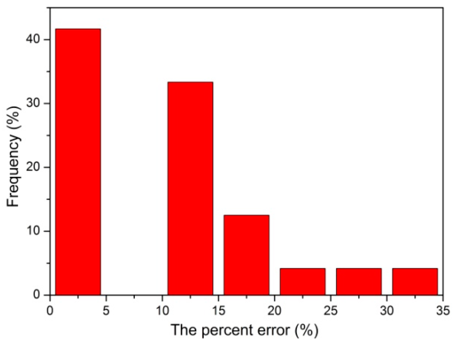
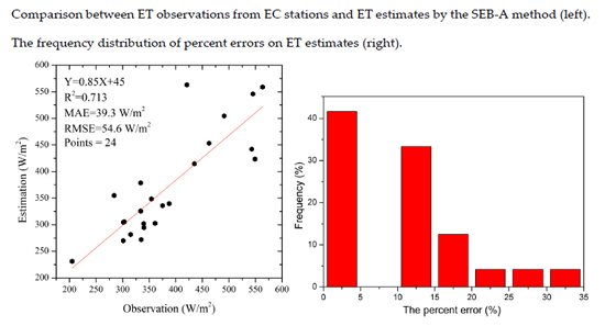
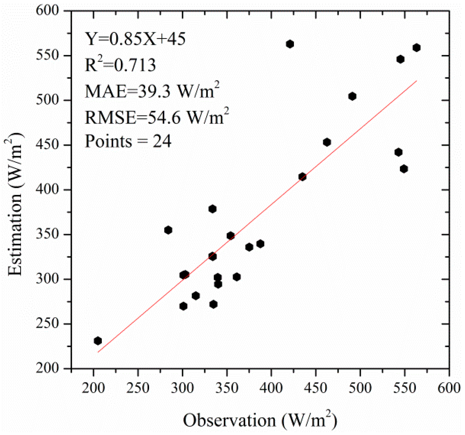
The study proposes the SEB-A method, which is innovative in that it considers the horizontal advection when applying the energy balance theory to estimate ET through remote sensing. The advantage of the SEB-A method is that it simplifies the ET process and regards the ET as regulated by two different driving forces: the local driving force and the exotic driving force. The local driving force is generated by radiation effects and can be described by the energy balance equation, whereas the exotic driving force is caused by the horizontal advection and can be expressed indirectly through ground-based EC observations. The idea makes the ET retrieval much simpler for the exact air aerodynamic resistance and for the quantification of the exotic ET. Model application and validation indicated that ET estimates from the SEB-A method had high accuracy, with an R² of 0.713, a MAE of 39.3 W/m² and an RMSE of 54.6 W/m² between estimates and measurements. In addition, ET estimates had percent errors within 20% at more than 80% of the locations and could well demonstrate ET differences caused by heterogeneous underlying surfaces. The sensitivity results showed that the SEB-A method requested accurate estimation of Rn − G, but it was insensitive to the difference between surface and air temperatures.

Since the influence of horizontal advection on ET is ubiquitous in practice, it is necessary to consider the exotic ET caused by the horizontal advection. The SEB-A method puts forward the way of utilizing ground-based EC measurements to quantify the exotic ET, which is verified with high accuracy. If remote sensing data and ground-based measurements including meteorological variables and surface fluxes are available, the SEB-A method can perform well. However, the method cannot work well when the ground-based measurements is insufficient.

References

1. Kothavala, Z.; Arain, M.A.; Black, T.A.; Verseghy, D. The simulation of energy, water vapor and carbon dioxide fluxes over common crops by the Canadian Land Surface Scheme (CLASS). Agric. For. Meteorol. 2005, 133, 89–108. [Google Scholar]
2. Anderson, M.C.; Norman, J.M.; Kustas, W.P.; Houborg, R.; Starks, P.J.; Agam, N. A thermal-based remote sensing technique for routine mapping of land-surface carbon, water and energy fluxes from field to regional scales. Remote Sens. Environ. 2008, 112, 4227–4241. [Google Scholar] [CrossRef]
3. Brutsaert, W. Hydrology: An Introduction; Cambridge University Press: New York, NY, USA, 2005. [Google Scholar]
4. Priestley, C.H.B.; Taylor, R.J. On the assessment of surface heat flux and evaporation using large-scale parameters. Mon. Weather Rev. 1972, 100, 81–92. [Google Scholar] [CrossRef]
5. Wang, S. Simulation of evapotranspiration and its response to plant water and CO2 transfer dynamics. J. Hydrometeorol. 2008, 9, 426–443. [Google Scholar] [CrossRef]
6. Xu, C.; Singh, V.; Chen, Y.; Chen, E. Evaporation and evapotranspiration. In Hydrology and Hydraulics; Singh, V., Ed.; Water Resource Publications: Michigan, MI, USA, 2008; Volume 6, pp. 229–269. [Google Scholar]
7. Cheng, C.-H.; Nnadi, F.; Liou, Y.-A.; Ma, Y.; Oguchi, T.; Chaubey, I.; Koch, M.; Thenkabail, P. A regional land use drought index for Florida. Remote Sens. 2015, 7, 17149–17167. [Google Scholar] [CrossRef]
8. Engman, E.T.; Gurney, R.J. Remote Sensing in Hydrology; Chapman and Hall: London, UK, 1991. [Google Scholar]
9. Liou, Y.A.; Kar, S.K. Evapotranspiration estimation with remote sensing and various surface energy balance algorithms-A review. Energies 2014, 7, 2821–2849. [Google Scholar] [CrossRef]
10. Sellers, P.J.; Dickinson, R.E.; Randall, D.A.; Betts, A.K.; Hall, F.G.; Berry, J.A.; Collatz, G.J.; Denning, A.S.; Mooney, H.A.; Nobre, C.A.; et al. Modeling the exchanges of energy, water, and carbon between continents and the atmosphere. Science 1997, 275, 502–509. [Google Scholar] [CrossRef] [PubMed]
11. Glenn, E.P.; Huete, A.R.; Nagler, P.L.; Hirschboeck, K.K.; Brown, P. Integrating remote sensing and ground methods to estimate evapotranspiration. Crit. Rev. Plant Sci. 2007, 26, 139–168. [Google Scholar] [CrossRef]
12. Kustas, W.; Anderson, M. Advances in thermal infrared remote sensing for land surface modeling. Agric. For. Meteorol. 2009, 149, 2071–2081. [Google Scholar] [CrossRef]
13. Shuttleworth, W.J. Putting the“ VAP” into evaporation. Hydrol. Earth Syst. Sci. 2007, 11, 210–244. [Google Scholar] [CrossRef]
14. Wang, K.; Dickinson, R.E. A review of global terrestrial evapotranspiration: Observation, modelling, climatology, and climatic variability. Rev. Geophys. 2012, 50, 1–54. [Google Scholar] [CrossRef]
15. Kalma, J.D.; McVicar, T.R.; McCabe, M.F. Estimating land surface evaporation: A review of methods using remotely sensed surface temperature data. Surv. Geophys. 2008, 29, 421–469. [Google Scholar] [CrossRef]
16. Li, Z.L.; Tang, R.; Wan, Z.; Bi, Y.; Zhou, C.; Tang, B.; Yan, G.; Zhang, X. A review of current methodologies for regional Evapotranspiration estimation from remotely sensed data. Sensors 2009, 9, 3801–3853. [Google Scholar] [CrossRef] [PubMed]
17. Liou, Y.-A.; Galantowicz, J.F.; England, A.W. A land surface process/radiobrightness model with coupled heat and moisture transport for prairie grassland. IEEE Trans. Geosci. Remote Sens. 1999, 37, 1848–1859. [Google Scholar] [CrossRef]
18. Kustas, W.P.; Norman, J.M. Evaluation of soil and vegetation heat flux predictions using a simple two-source model with radiometric temperatures for partial canopy cover. Agric. For. Meteorol. 1999, 94, 13–29. [Google Scholar] [CrossRef]
19. Bhattacharya, B.K.; Mallick, K.; Patel, N.K.; Parihar, J.S. Regional clear sky evapotranspiration over agricultural land using remote sensing data from Indian geostationary meteorological satellite. J. Hydrol. 2010, 387, 65–80. [Google Scholar] [CrossRef]
20. Norman, J.M.; Kustas, W.P.; Humes, K.S. Source approach for estimating soil and vegetation energy fluxes in observations of directional radiometric surface temperature. Agric. For. Meteorol. 1995, 77, 263–293. [Google Scholar] [CrossRef]
21. Timmermans, W.J.; Kustas, W.P.; Anderson, M.C.; French, A.N. An intercomparison of the Surface Energy Balance Algorithm for Land (SEBAL) and the Two-Source Energy Balance (TSEB) modeling schemes. Remote Sens. Environ. 2007, 108, 369–384. [Google Scholar] [CrossRef]
22. Yang, Y.; Su, H.; Zhang, R.; Tian, J.; Li, L. An enhanced two-source evapotranspiration model for land (ETEML): Algorithm and evaluation. Remote Sens. Environ. 2015, 168, 54–65. [Google Scholar] [CrossRef]
23. Spronken-smith, R.A.; Oke, T.R.; Lowry, W.P. Advection and the surface energy balance across and irrigated urban park. Int. J. Climatol. 2000, 1047, 1033–1047. [Google Scholar] [CrossRef]
24. Masson, V.; Grimmond, C.S.B.; Oke, T.R. Evaluation of the town energy balance (TEB) scheme with direct measurements from dry districts in two cities. Am. Meteorol. Soc. 2002, 41, 1011–1026. [Google Scholar]
25. Wilson, K.; Goldstein, A.; Falge, E.; Aubinet, M.; Baldocchi, D.; Berbigier, P.; Bernhofer, C.; Ceulemans, R.; Dolman, H.; Field, C.; et al. Energy balance closure at FLUXNET sites. Agric. For. Meteorol. 2002, 113, 223–243. [Google Scholar] [CrossRef]
26. Tian, J.; Zhang, R.; Sun, X.; Zhu, Z.; Zhou, Y. Study of a model for correcting the effects of horizontal advection on surface fluxes measurement based on remote sensing. Sci. China Ser. D Earth Sci. 2006, 49, 273–280. [Google Scholar] [CrossRef]
27. Yang, Y.; Su, H.; Zhang, R.; Xia, J. Revised advection-aridity evaporation model. J. Hydrol. Eng. 2012, 18, 655–664. [Google Scholar] [CrossRef]
28. Jia, J.; Zhao, W.; Li, S. Regional evapotranspiration rate of oasis and surrounding desert. Hydrol. Process. 2013, 27, 3409–3414. [Google Scholar] [CrossRef]
29. Lian, J.; Huang, M. Comparison of three remote sensing based models to estimate evapotranspiration in an oasis-desert region. Agric. Water Manag. 2016, 165, 153–162. [Google Scholar] [CrossRef]
30. French, A.N.; Jacob, F.; Anderson, M.C.; Kustas, W.P.; Timmermans, W.; Gieske, A.; Su, Z.; Su, H.; McCabe, M.F.; Li, F.; Prueger, J.; Brunsell, N. Surface energy fluxes with the advanced spaceborne thermal Emission and reflection radiometer (ASTER) at the Iowa 2002 SMACEX site (USA). Remote Sens. Environ. 2005, 99, 55–65. [Google Scholar] [CrossRef]
31. Qiang, L.; Jianguang, W.; Shengbiao, W.; Ying, Q. Albedo Dataset in 30 m-Resolution in the Heihe River Basin in 2012; Heihe Plan Science Data Center: Lanzhou, China, 2014. [Google Scholar]
32. Li, H.; Sun, D.; Yu, Y.; Wang, H.; Liu, Y.; Liu, Q.; Du, Y.; Wang, H.; Cao, B. Evaluation of the VIIRS and MODIS LST products in an arid area of Northwest China. Remote Sens. Environ. 2014, 142, 111–121. [Google Scholar] [CrossRef]
33. Li, X.; Cheng, G.; Liu, S.; Xiao, Q.; Ma, M.; Jin, R.; Che, T.; Liu, Q.; Wang, W.; Qi, Y.; et al. Heihe watershed allied telemetry experimental research (HiWATER): Scientific objectives and experimental design. Bull. Am. Meteorol. Soc. 2013, 94, 1145–1160. [Google Scholar] [CrossRef]
34. Zhang, R.; Rong, Y.; Tian, J.; Su, H.; Li, Z.-L.; Liu, S. A remote sensing method for estimating surface air temperature and surface vapor pressure on a regional scale. Remote Sens. 2015, 7, 6005–6025. [Google Scholar] [CrossRef]
35. Bastiaanssen, W.G.M.; Menenti, M.; Feddes, R.A.; Holtslag, A.A.M. A remote sensing surface energy balance algorithm for land (SEBAL). 1. Formulation. J. Hydrol. 1998, 212, 198–212. [Google Scholar] [CrossRef]
36. Su, Z. The Surface Energy Balance System (SEBS) for estimation of turbulent heat fluxes. Hydrol. Earth Syst. Sci. 2002, 6, 85–100. [Google Scholar] [CrossRef]
37. Zhang, R.; Sun, X.; Zhu, Z.; Su, H.; Tang, X. A remote sensing model for monitoring soil evaporation based on differential thermal inertia and its validation. Sci. China Ser. D Earth Sci. 2003, 46, 342–355. [Google Scholar]
38. Burden, R.L.; Faires, J.D. Numerical Analysis; Brooks/Cole: Boston, MA, USA, 2001. [Google Scholar]
39. Zhang, M.; Ma, M.; Wang, X. HiWATER: Land Cover Map in the Core Experimental Area of Flux Observation Matrix; Heihe Plan Science Data Center: Lanzhou, China, 2014. [Google Scholar]
40. Wang, Y.C.; Chang, T.; Liou, Y.A. Terrain correction for increasing the evapotranspiration estimation accuracy in a mountainous watershed. IEEE Geosci. Remote Sens. Lett. 2010, 7, 352–356. [Google Scholar] [CrossRef]
Figure 1. Location of the study area including land use status and 17 ground-based stations.
Remotesensing 08 00644 g001
Figure 2. The principle of the surface energy balance-advection (SEB-A) method.
Remotesensing 08 00644 g002
Figure 3. ET estimated by the SEB-A method on: 10 July 2012 (a); 11 August 2012 (b); and 27 August 2012 (c).
Remotesensing 08 00644 g003
Figure 4. Comparison between ET observations from EC stations and ET estimates by the SEB-A method.
Remotesensing 08 00644 g004
Figure 5. The frequency distribution of percent errors on ET estimates.
Remotesensing 08 00644 g005