
Quantifying Freshwater Mass Balance in the Central Tibetan Plateau by Integrating Satellite Remote Sensing, Altimetry, and Gravimetry

 ,
,  ,
,  ,
,
Abstract
:
1. Introduction
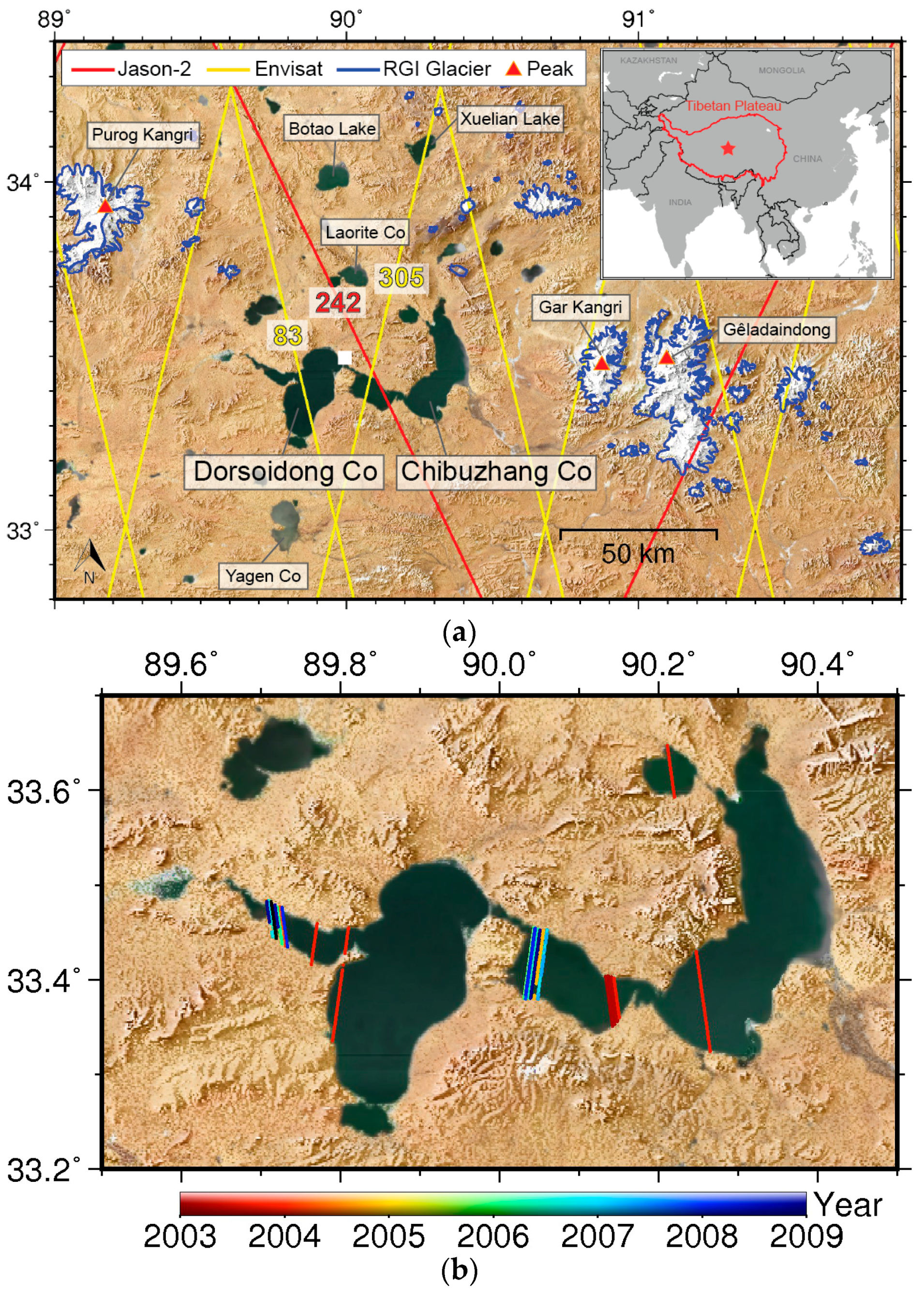
2. Study Area
3. Satellite Data and Processing Method
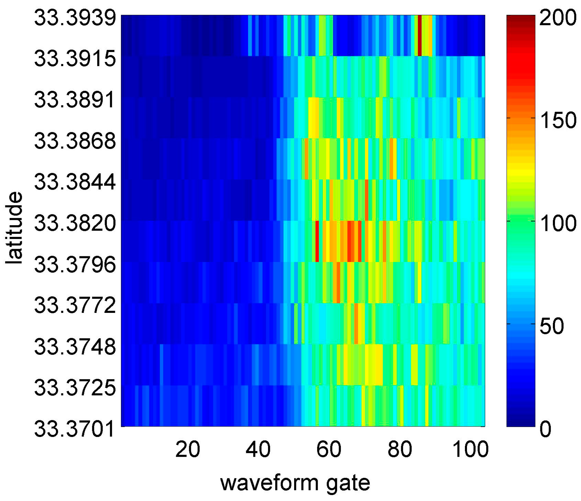
3.1. Radar and Laser Altimetry
3.2. Optical Remote Sensing and Water Detection
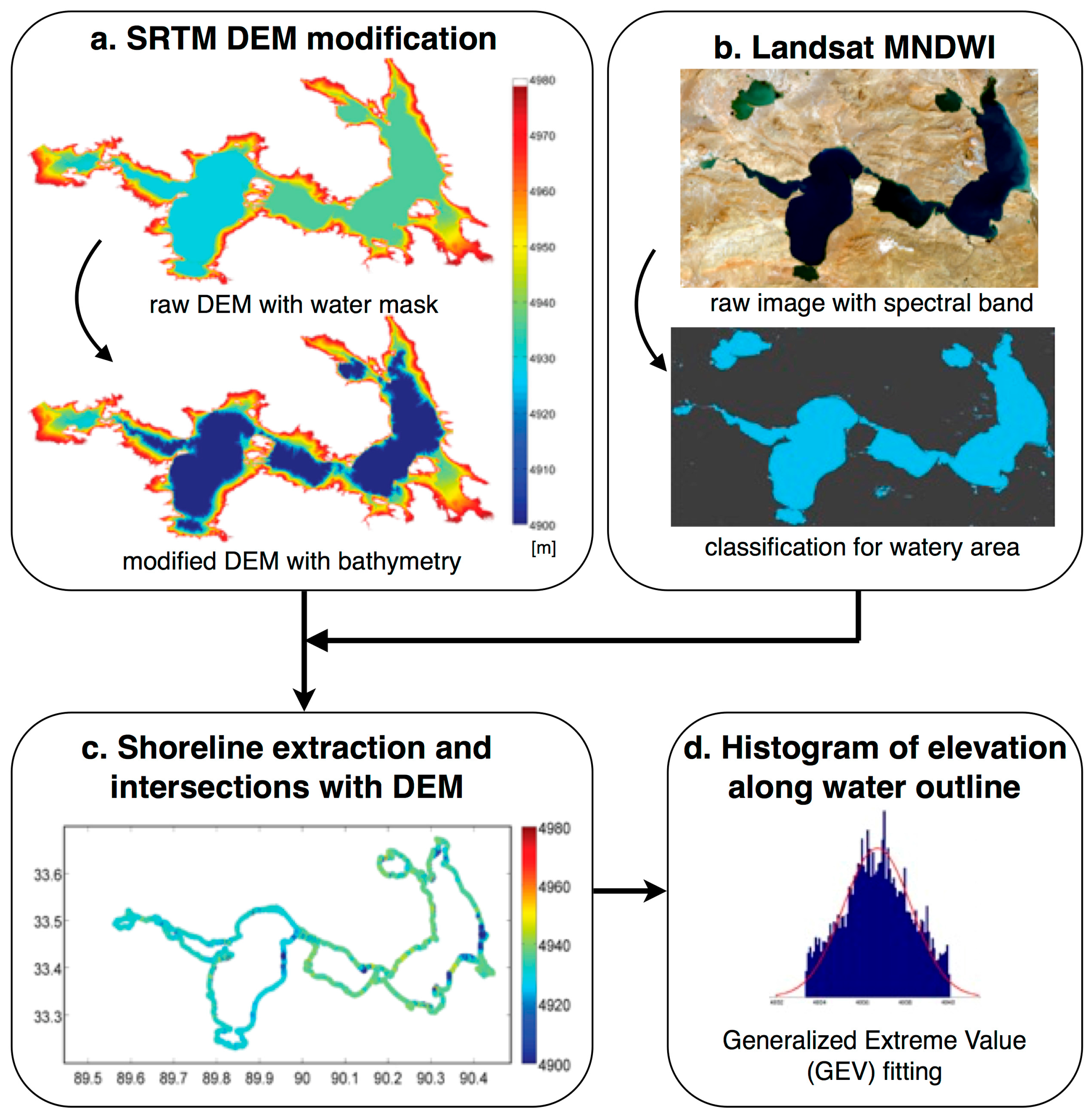
3.3. From Water Area to Water Level Estimate
3.4. GRACE Gravimetry Mission Data
3.5. TRMM Precipitation Record
4. Results
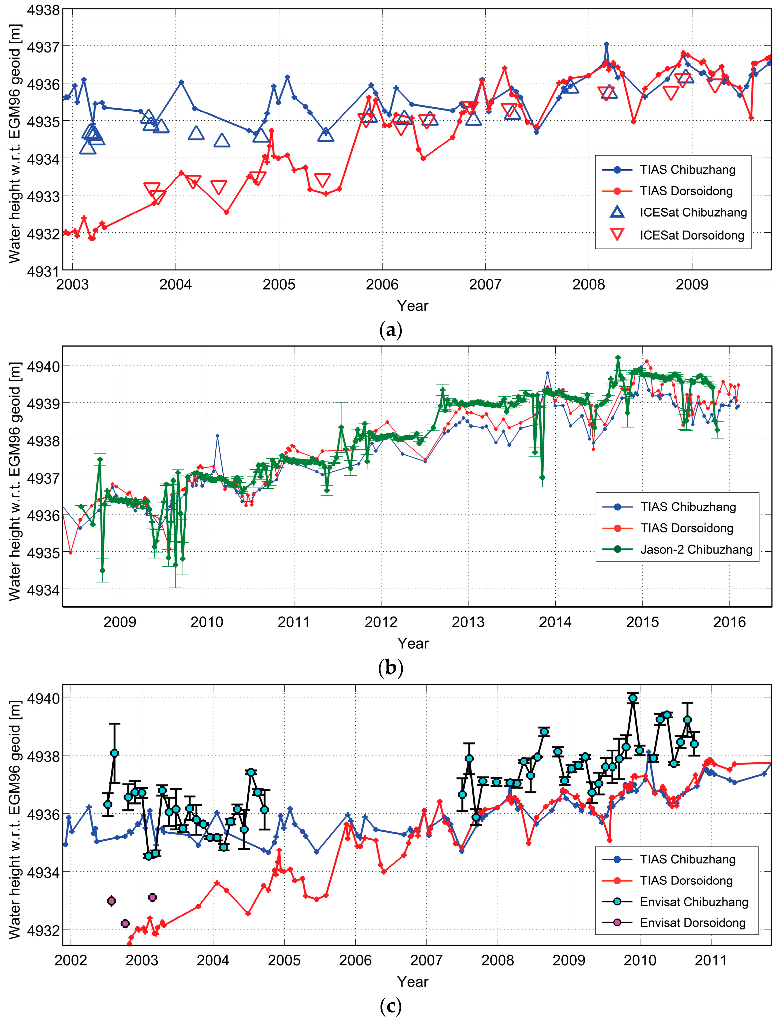
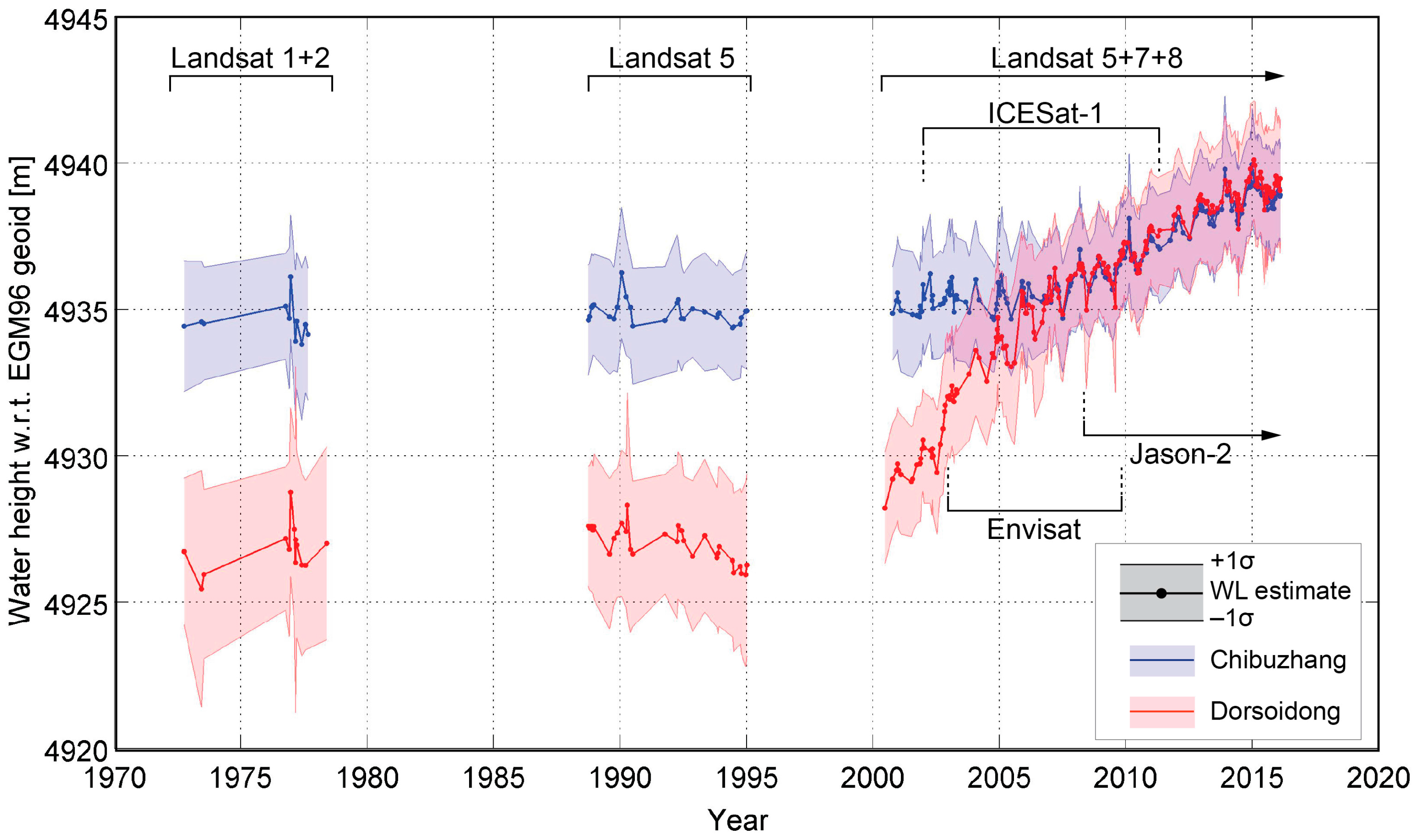
4.1. Validtion of Altimetry Results
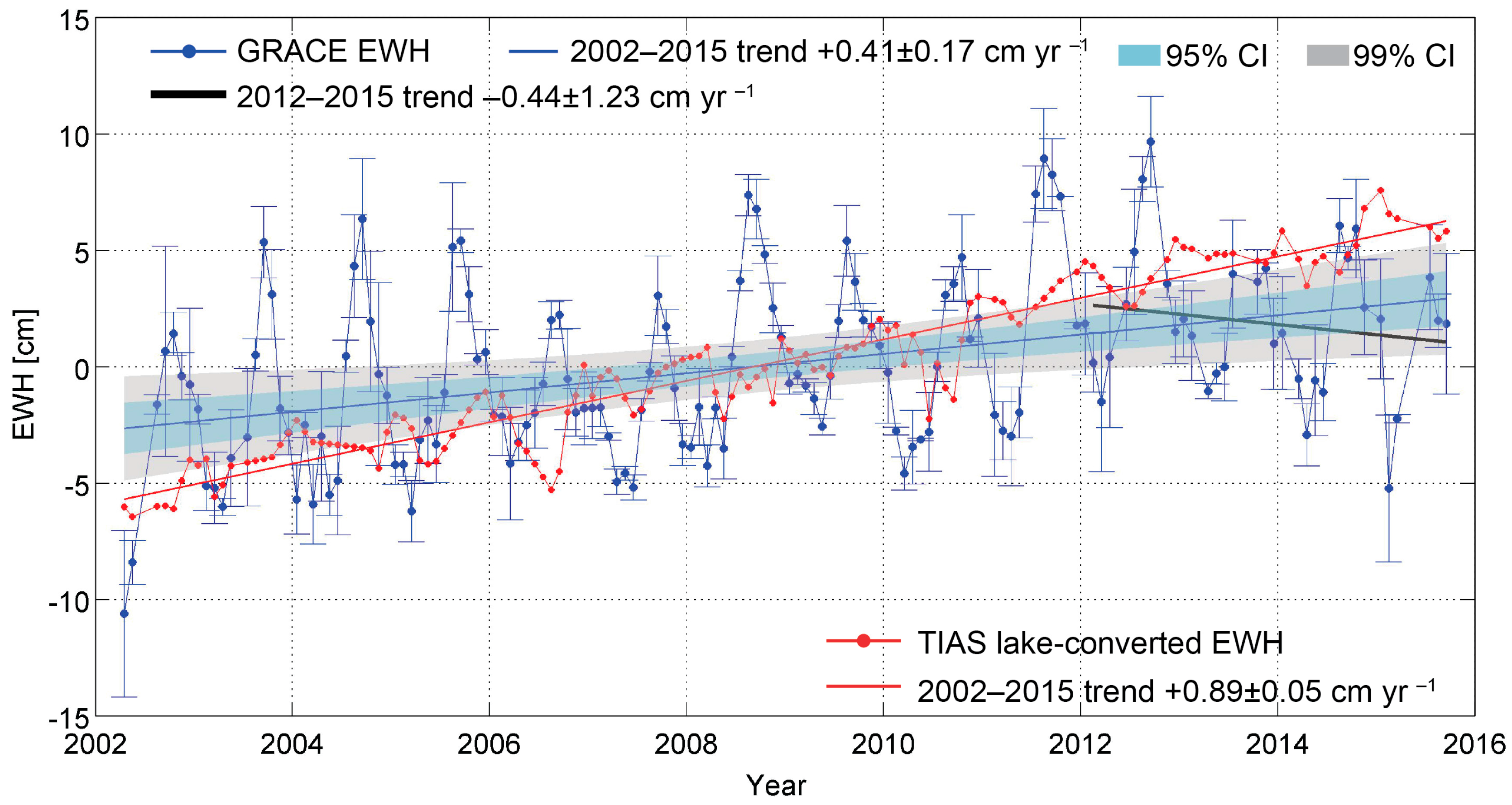
4.2. Quantification of Water Volume Change
5. Discussions
6. Conclusions
Acknowledgments
Author Contributions
Conflicts of Interest
References
- Fang, Y.; Cheng, W.; Zhang, Y.; Wang, N.; Zhao, S.; Zhou, C.; Chen, X.; Bao, A. Changes in inland lakes on the Tibetan Plateau over the past 40 years. J. Geogr. Sci. 2016, 26, 415–438. [Google Scholar] [CrossRef]
- Khandu, K.; Forootan, E.; Schumacher, M.; Awange, J.L.; Müller Schmied, H. Exploring the influence of precipitation extremes and human water use on total water storage (TWS) changes in the Ganges-Brahmaputra-Meghna River Basin. Water Resour. Res. 2016, 52, 2240–2258. [Google Scholar] [CrossRef]
- Liu, X.; Chen, B. Climatic warming in the Tibetan Plateau during recent decades. Int. J. Climatol. 2000, 20, 1729–1742. [Google Scholar] [CrossRef]
- Xu, B.; Cao, J.; Hansen, J.; Yao, T.; Joswia, D.R.; Wang, N.; Wu, G.; Wang, M.; Zhao, H.; Yang, W.; et al. Black soot and the survival of Tibetan glaciers. Proc. Natl. Acad. Sci. USA 2009, 106, 22114–22118. [Google Scholar] [CrossRef] [PubMed]
- Tseng, K.H.; Shum, C.K.; Lee, H.; Duan, J.B.; Kuo, C.Y.; Song, S.L.; Zhu, W.Y. Satellite observed environmental changes over the Qinghai-Tibetan Plateau. Terr. Atmos. Ocean. Sci. 2011, 22, 229–239. [Google Scholar] [CrossRef]
- Song, C.; Huang, B.; Richards, K.; Ke, L.; Hien Phan, V. Accelerated lake expansion on the Tibetan Plateau in the 2000s: Induced by glacial melting or other processes? Water Resour. Res. 2014, 50, 3170–3186. [Google Scholar] [CrossRef]
- Zhang, G.; Yao, T.; Xie, H.; Kang, S.; Lei, Y. Increased mass over the Tibetan Plateau: From lakes or glaciers? Geophys. Res. Lett. 2013, 40, 2125–2130. [Google Scholar] [CrossRef]
- Tapley, B.D.; Bettadpur, S.; Ries, J.C.; Thompson, P.F.; Watkins, M.M. GRACE measurements of mass variability in the Earth system. Science 2004, 305, 503–505. [Google Scholar] [CrossRef] [PubMed]
- Moore, P.; Williams, S.D.P. Integration of altimetric lake levels and GRACE gravimetry over Africa: Inferences for terrestrial water storage change 2003–2011. Water Resour. Res. 2014, 50, 9696–9720. [Google Scholar] [CrossRef]
- Medina, C.; Gomez-Enri, J.; Alonso, J.J.; Villares, P. Water volume variations in Lake Izabal (Guatemala) from in situ measurements and ENVISAT Radar Altimeter (RA-2) and Advanced Synthetic Aperture Radar (ASAR) data products. J. Hydrol. 2010, 382, 34–48. [Google Scholar] [CrossRef]
- Baup, F.; Frappart, F.; Maubant, J. Combining high-resolution satellite images and altimetry to estimate the volume of small lakes. Hydrol. Earth Syst. Sci. 2014, 18, 2007–2020. [Google Scholar] [CrossRef]
- Tseng, K.H.; Shum, C.K.; Kim, J.W.; Wang, X.; Zhu, K.; Cheng, X. Integrating Landsat Imageries and Digital Elevation Models to Infer Water Level Change in Hoover Dam. IEEE J. Sel. Top. Appl. Earth Obs. Remote Sens. 2015, 1–14. [Google Scholar] [CrossRef]
- Song, C.; Sheng, Y. Contrasting evolution patterns between glacier-fed and non-glacier-fed lakes in the Tanggula Mountains and climate cause analysis. Clim. Chang. 2015, 135, 493–507. [Google Scholar] [CrossRef]
- Zhang, P.Z.; Shen, Z.; Wang, M.; Gan, W.; Bürgmann, R.; Molnar, P.; Wang, Q.; Niu, Z.; Sun, J.; Wu, J.; et al. Continuous deformation of the Tibetan Plateau from global positioning system data. Geology 2004, 32, 809–812. [Google Scholar] [CrossRef]
- Zhang, J.; Braaten, D.A.; Li, X.; Tao, F. An Inventory of Glacier Changes between 1973 and 2011 for the Geladandong Mountain Area, China; European Geosciences Union: Munich, Germany, 2013. [Google Scholar]
- Ye, Q.; Kang, S.; Chen, F.; Wang, J. Monitoring glacier variations on Geladandong mountain 2013, central Tibetan Plateau, from 1969 to 2002 using remote-sensing and GIS technologies. J. Glaciol. 2006, 52, 537–545. [Google Scholar] [CrossRef]
- Zhang, Y.; Yao, T.; Ma, Y. Climatic changes have led to significant expansion of lakes in Xizang (Tibet) since 1995. Sci. Cold Arid Reg. 2011, 3, 463–467. [Google Scholar]
- Zhang, Y.; Liu, S.Y.; Xu, J.L.; Shangguan, D.H. Glacier change and glacier runoff variation in the Tuotuo River basin, the source region of Yangtze River in western China. Environ. Geol. 2008, 56, 59–68. [Google Scholar] [CrossRef]
- Pfeffer, W.T.; Arendt, A.A.; Bliss, A.; Bolch, T.; Cogley, J.G.; Gardner, A.S.; Hagen, J.O.; Hock, R.; Kaser, G.; Kienholz, C.; et al. The Randolph Glacier Inventory: A globally complete inventory of glaciers. J. Glaciol. 2014, 60, 537–552. [Google Scholar] [CrossRef]
- Brown, G.S. The average impulse response of a rough surface and its applications. IEEE Trans. Antennas Propag. 1977, 25, 67–74. [Google Scholar] [CrossRef]
- Van der Veen, C.J. Interpretation of short-term ice-sheet elevation changes inferred from satellite altimetry. Clim. Chang. 1993, 23, 383–405. [Google Scholar] [CrossRef]
- Ekholm, S.; Forsberg, R.; Brozena, J.M. Accuracy of satellite altimeter elevations over the Greenland ice sheet. J. Geophys. Res. Oceans 1995, 100, 2687–2696. [Google Scholar] [CrossRef]
- Kouraev, A.V.; Semovski, S.V.; Shimaraev, M.N.; Mognard, N.M.; Légresy, B.; Remy, F. Observations of Lake Baikal ice from satellite altimetry and radiometry. Remote Sens. Environ. 2007, 108, 240–253. [Google Scholar] [CrossRef]
- Tseng, K.H.; Shum, C.K.; Yi, Y.; Emery, W.J.; Kuo, C.Y.; Lee, H.; Wang, H. The improved retrieval of coastal sea surface heights by retracking modified radar altimetry waveforms. IEEE Trans. Geosci. Remote Sens. 2014, 52, 991–1001. [Google Scholar] [CrossRef]
- Berry, P.A.M.; Garlick, J.D.; Freeman, J.A.; Mathers, E.L. Global inland water monitoring from multi-mission altimetry. Geophys. Res. Lett. 2005, 32. [Google Scholar] [CrossRef]
- Lee, H.; Shum, C.K.; Tseng, K.H.; Huang, Z.; Sohn, H.G. Elevation changes of Bering Glacier System, Alaska, from 1992 to 2010, observed by satellite radar altimetry. Remote Sens. Environ. 2013, 132, 40–48. [Google Scholar] [CrossRef]
- Liu, G.; Schwartz, F.W.; Tseng, K.H.; Shum, C.K. Discharge and water-depth estimates for ungauged rivers: Combining hydrologic, hydraulic, and inverse modeling with stage and water-area measurements from satellites. Water Resour. Res. 2015, 51, 6017–6035. [Google Scholar] [CrossRef]
- Uebbing, B.; Kusche, J.; Forootan, E. Waveform retracking for improving level estimations from TOPEX/Poseidon, Jason-1, and Jason-2 Altimetry Observations over African Lakes. IEEE Trans. Geosci. Remote Sens. 2015, 53, 2211–2224. [Google Scholar] [CrossRef]
- Kuo, C.Y.; Cheng, Y.J.; Lan, W.H.; Kao, H.C. Monitoring Vertical Land Motions in Southwestern Taiwan with Retracked Topex/Poseidon and Jason-2 Satellite Altimetry. Remote Sens. 2015, 7, 3808–3825. [Google Scholar] [CrossRef]
- Shum, C.K.; Ries, J.C.; Tapley, B.D. The accuracy and applications of satellite altimetry. Geophys. J. Int. 1995, 121, 321–336. [Google Scholar] [CrossRef]
- Tseng, K.H.; Shum, C.K.; Yi, Y.; Fok, H.S.; Kuo, C.Y.; Lee, H.; Cheng, X.; Wang, X. Envisat altimetry radar waveform retracking of quasi-specular echoes over the ice-covered Qinghai lake. Terr. Atmos. Ocean. Sci. 2013, 24, 615–627. [Google Scholar] [CrossRef]
- Kuo, C.Y.; Kao, H.C. Retracked Jason-2 altimetry over small water bodies: Case study of Bajhang River, Taiwan. Mar. Geod. 2011, 34, 382–392. [Google Scholar] [CrossRef]
- Sulistioadi, Y.B.; Tseng, K.H.; Shum, C.K.; Hidayat, H.; Sumaryono, M.; Suhardiman, A.; Setiawan, F.; Sunarso, S. Satellite radar altimetry for monitoring small rivers and lakes in Indonesia. Hydrol. Earth Syst. Sci. 2015, 19, 341–359. [Google Scholar] [CrossRef]
- Zelli, C. ENVISAT RA-2 advanced radar altimeter: Instrument design and pre-launch performance assessment review. Acta Astronaut. 1999, 44, 323–333. [Google Scholar] [CrossRef]
- Frappart, F.; Calmant, S.; Cauhopé, M.; Seyler, F.; Cazenave, A. Preliminary results of ENVISAT RA-2-derived water levels validation over the Amazon basin. Remote Sens. Environ. 2006, 100, 252–264. [Google Scholar] [CrossRef]
- Khaki, M.; Forootan, E.; Sharifi, M.A. Satellite radar altimetry waveform retracking over the Caspian Sea. Int. J. Remote Sens. 2014, 35, 6329–6356. [Google Scholar] [CrossRef]
- Guo, J.; Chang, X.; Gao, Y.; Sun, J.; Hwang, C. Lake level variations monitored with satellite altimetry waveform retracking. IEEE J. Sel. Top. Appl. Earth Obs. Remote Sens. 2009, 2, 80–86. [Google Scholar] [CrossRef]
- Lee, H.; Shum, C.K.; Tseng, K.H.; Guo, J.Y.; Kuo, C.Y. Present-day lake level variation from ENVISAT Altimetry over the northeastern Qinghai-Tibetan Plateau: Links with precipitation and temperature. J. Terr. Atmos. Ocean Sci. 2011, 22, 169–175. [Google Scholar] [CrossRef]
- Lambin, J.; Morrow, R.; Fu, L.L.; Willis, J.K.; Bonekamp, H.; Lillibridge, J.; Perbos, J.; Zaouche, G.; Vaze, P.; Bannoura, W.; et al. The OSTM/Jason-2 mission. Mar. Geod. 2010, 33, 4–25. [Google Scholar] [CrossRef]
- Schutz, B.E.; Zwally, H.J.; Shuman, C.A.; Hancock, D.; DiMarzio, J.P. Overview of the ICESat mission. Geophys. Res. Lett. 2005, 32. [Google Scholar] [CrossRef]
- Abshire, J.B.; Sun, X.; Riris, H.; Sirota, J.M.; McGarry, J.F.; Palm, S.; Yi, D.; Liiva, P. Geoscience laser altimeter system (GLAS) on the ICESat mission: On-orbit measurement performance. Geophys. Res. Lett. 2005, 32, L21S02. [Google Scholar] [CrossRef]
- NASA’s Earth Observing System Clearing House (ECHO) Online Portal. Available online: http://reverb.echo.nasa.gov (accessed on 10 May 2016).
- EarthExplorer. Available online: http://earthexplorer.usgs.gov (accessed on 10 May 2016).
- Chander, G.; Markham, B.L.; Helder, D.L. Summary of current radiometric calibration coefficients for Landsat MSS, TM, ETM+, and EO-1 ALI sensors. Remote Sens. Environ. 2009, 113, 893–903. [Google Scholar] [CrossRef]
- USGS. Using the USGS Landsat 8 Product. Available online: http://landsat.usgs.gov/Landsat8_Using_Product.php (accessed on 10 May 2016).
- Burns, P.; Nolin, A. Using atmospherically-corrected Landsat imagery to measure glacier area change in the Cordillera Blanca, Peru from 1987 to 2010. Remote Sens. Environ. 2014, 140, 165–178. [Google Scholar] [CrossRef]
- Singh, A. Review article digital change detection techniques using remotely-sensed data. Int. J. Remote Sens. 1989, 10, 989–1003. [Google Scholar] [CrossRef]
- Xu, H. Modification of normalized difference water index (NDWI) to enhance open water features in remotely sensed imagery. Int. J. Remote Sens. 2006, 27, 3025–3033. [Google Scholar] [CrossRef]
- McFeeters, S.K. The use of the Normalized Difference Water Index (NDWI) in the delineation of open water features. Int. J. Remote Sens. 1996, 17, 1425–1432. [Google Scholar] [CrossRef]
- Ries, J.C.; Bettadpur, S.; Poole, S.; Richter, T. Mean background gravity fields for GRACE processing. In Proceedings of the GRACE Science Team Meeting, Austin, TX, USA, 8–10 August 2011.
- Duan, X.J.; Guo, J.Y.; Shum, C.K.; Van Der Wal, W. On the postprocessing removal of correlated errors in GRACE temporal gravity field solutions. J. Geod. 2009, 83, 1095–1106. [Google Scholar] [CrossRef]
- Guo, J.Y.; Duan, X.J.; Shum, C.K. Non-isotropic Gaussian smoothing and leakage reduction for determining mass changes over land and ocean using GRACE data. Geophys. J. Int. 2010, 181, 290–302. [Google Scholar] [CrossRef]
- Cheng, M.K.; Tapley, B.D.; Ries, J.C. Deceleration in the Earth’s oblateness. J. Geophys. Res. 2013, 118, 1–8. [Google Scholar] [CrossRef]
- Swenson, S.; Chambers, D.; Wahr, J. Estimating geocenter variations from a combination of GRACE and ocean model output. J. Geophys. Res. Solid Earth 2008, 113, B08410. [Google Scholar] [CrossRef]
- Ivins, E.R.; James, T.S.; Wahr, J.; Schrama, E.J.O.; Landerer, F.W.; Simon, K.M. Antarctic contribution to sea level rise observed by GRACE with improved GIA correction. J. Geophys. Res. Solid Earth 2013, 118, 3126–3141. [Google Scholar] [CrossRef]
- Forootan, E.; Kusche, J.; Loth, I.; Schuh, W.D.; Eicker, A.; Awange, J.; Longuevergne, L.; Diekkrüger, B.; Schmidt, M.; Shum, C.K. Multivariate prediction of total water storage changes over West Africa from multi-satellite data. Surv. Geophys. 2014, 35, 913–940. [Google Scholar] [CrossRef]
- Huffman, G.J.; Bolvin, D.T.; Nelkin, E.J.; Wolff, D.B.; Adler, R.F.; Gu, G.; Hong, Y.; Bowman, K.P.; Stocker, E.F. The TRMM multisatellite precipitation analysis (TMPA): Quasi-global, multiyear, combined-sensor precipitation estimates at fine scales. J. Hydrometeorol. 2007, 8, 38–55. [Google Scholar] [CrossRef]


| Landsat # (Sensor) | 1 (MSS) | 2 (MSS) | 5 (TM) | 7 (TM) | 8 (OLI) |
|---|---|---|---|---|---|
| Green Band | 4 | 4 | 2 | 2 | 3 |
| MIR Band | 7 | 7 | 5 | 5 | 6 |
| Index Threshold | 0.4 | 0.4 | 0.2 | 0.2 | 0.4 |
| Chibuzhang Dorsoidong | TIAS | ICESat | Jason-2 | Envisat |
|---|---|---|---|---|
| TIAS | -- | 0.30/0.90 | 0.49/0.93 | 1.02/0.65 |
| ICESat | 0.42/0.98 | -- | N/A | 0.54/0.93 |
| Jason-2 | 0.48/0.94 | N/A | -- | 0.68/0.57 |
| Envisat | N/A | N/A | N/A | -- |
© 2016 by the authors; licensee MDPI, Basel, Switzerland. This article is an open access article distributed under the terms and conditions of the Creative Commons Attribution (CC-BY) license (http://creativecommons.org/licenses/by/4.0/).
Share and Cite
Tseng, K.-H.; Chang, C.-P.; Shum, C.K.; Kuo, C.-Y.; Liu, K.-T.; Shang, K.; Jia, Y.; Sun, J. Quantifying Freshwater Mass Balance in the Central Tibetan Plateau by Integrating Satellite Remote Sensing, Altimetry, and Gravimetry. Remote Sens. 2016, 8, 441. https://doi.org/10.3390/rs8060441
Tseng K-H, Chang C-P, Shum CK, Kuo C-Y, Liu K-T, Shang K, Jia Y, Sun J. Quantifying Freshwater Mass Balance in the Central Tibetan Plateau by Integrating Satellite Remote Sensing, Altimetry, and Gravimetry. Remote Sensing. 2016; 8(6):441. https://doi.org/10.3390/rs8060441
Chicago/Turabian StyleTseng, Kuo-Hsin, Chung-Pai Chang, C. K. Shum, Chung-Yen Kuo, Kuan-Ting Liu, Kun Shang, Yuanyuan Jia, and Jian Sun. 2016. "Quantifying Freshwater Mass Balance in the Central Tibetan Plateau by Integrating Satellite Remote Sensing, Altimetry, and Gravimetry" Remote Sensing 8, no. 6: 441. https://doi.org/10.3390/rs8060441
APA StyleTseng, K.-H., Chang, C.-P., Shum, C. K., Kuo, C.-Y., Liu, K.-T., Shang, K., Jia, Y., & Sun, J. (2016). Quantifying Freshwater Mass Balance in the Central Tibetan Plateau by Integrating Satellite Remote Sensing, Altimetry, and Gravimetry. Remote Sensing, 8(6), 441. https://doi.org/10.3390/rs8060441