Characterizing Pavement Surface Distress Conditions with Hyper-Spatial Resolution Natural Color Aerial Photography

Abstract

Roadway pavement surface distress information is critical for effective pavement asset management, and subsequently, transportation management agencies at all levels (i.e., federal, state, and local) dedicate a large amount of time and money to routinely evaluate pavement surface distress conditions as the core of their asset management programs. However, currently adopted ground-based evaluation methods for pavement surface conditions have many disadvantages, like being time-consuming and expensive. Aircraft-based evaluation methods, although getting more attention, have not been used for any operational evaluation programs yet because the acquired images lack the spatial resolution to resolve finer scale pavement surface distresses. Hyper-spatial resolution natural color aerial photography (HSR-AP) provides a potential method for collecting pavement surface distress information that can supplement or substitute for currently adopted evaluation methods. Using roadway pavement sections located in the State of New Mexico as an example, this research explored the utility of aerial triangulation (AT) technique and HSR-AP acquired from a low-altitude and low-cost small-unmanned aircraft system (S-UAS), in this case a tethered helium weather balloon, to permit characterization of detailed pavement surface distress conditions. The Wilcoxon Signed Rank test, Mann-Whitney U test, and visual comparison were used to compare detailed pavement surface distress rates measured from HSR-AP derived products (orthophotos and digital surface models generated from AT) with reference distress rates manually collected on the ground using standard protocols. The results reveal that S-UAS based hyper-spatial resolution imaging and AT techniques can provide detailed and reliable primary observations suitable for characterizing detailed pavement surface distress conditions comparable to the ground-based manual measurement, which lays the foundation for the future application of HSR-AP for automated detection and assessment of detailed pavement surface distress conditions.

1. Introduction

As one of the most critical types of transportation infrastructure, roadways provide a foundation to the performance of all national economies, delivering a wide range of economic and social benefits [1]. In most countries, roadways are the primary transport mode for both freight and passengers [1,2,3,4]. Similar to other types of transportation infrastructure, roads deteriorate over time due to various factors such as age, traffic load, and weather conditions [5]. The serviceability of roads (i.e., the ability of a road to serve traffic) primarily depends on pavement surface conditions, and subsequently, road management agencies at all levels (i.e., federal, state, and local) devote large amounts of time and money to routinely evaluate pavement surface conditions as the core of their asset management programs. These pavement surface condition data are used by these agencies to make maintenance and repair decisions.

Historically, pavement evaluation was commonly performed with “boots on the ground” by having experts visually inspect the surface conditions with subjective judgment [6]. Pavement surface conditions were observed and recorded by inspectors in the field and the hand-written data was later inputted into a computer database. In the 1980s, vehicle-mounted electronic sensors (e.g., video cameras, digital cameras, and laser sensors) at a fine enough resolution emerged and were used for automated pavement surface evaluation [7,8,9,10]. Both manual observation and automated observation methods are classified as ground-based evaluation methods because the evaluation action occurs from the ground. Ground-based evaluation methods can collect detailed pavement surface condition data for various types of distresses (e.g., alligator cracking and transverse cracking). However, these methods are expensive [11], labor-intensive (manual observation only) [9,10,12,13,14,15], time-consuming [10], tedious [16], subjective (manual observation only) [17,18,19], potentially dangerous to inspectors in the hazardous roadway environment [10], require specialized staff on a regular basis [20], and can exhibit a high degree of variability [21], thereby causing inconsistencies in surveyed data over space and across evaluation [22]. In addition, data collected on the ground serves only a single purpose (i.e., pavement surface evaluation) and cannot be shared with other government agencies (e.g., U.S. Geological Survey) to reduce the cost [22].

Another method to evaluate pavement surface is through airborne observation. Airborne methods require deploying cameras (both analog and digital) on aircraft that can fly over pavement sections. Airborne remote sensing techniques, also known as aircraft-based evaluation, is getting more attention because of its synoptic coverage [23], although it has not been used for operational evaluation programs to the authors’ knowledge. The resulting aerial images, which typically have high-spatial resolutions ranging from 0.075 m (3 in) to 1 m, can be used to evaluate the overall condition of pavement surfaces in a more rapid, cost-effective (data can be shared with other government agencies), and safer manner [22,24]. However, the spatial resolutions of these images limit the ability to detect and assess fine and detailed defects such as individual cracks on a pavement surface because most cracks have widths less than 0.01 m [25]. Although visual interpretation of large scale (e.g., 1:100) panchromatic analog aerial photographs can be used to identify untreated cracks and other high-contrast pavement defects such as patching and bleeding, extremely high cost and limited compatibility with modern image processing techniques ultimately prevent the further exploration of their applications for pavement surface evaluation [26,27,28].

The above literature reveals the actual obstacle for using digital aerial images for detailed pavement surface distress evaluation is the spatial resolution is too coarse to resolve detailed distresses, which often manifest at the millimeter scale. Recent advances in remote sensing have enabled us to effectively collect hyper-spatial resolution (sub-centimeter or sub-inch) natural color aerial photography (HSR-AP) at a low cost. HSR-AP has been used to facilitate research in many fields, such as archaeology [29], ecology [30,31,32], zoology [33], emergency management [34], vegetation and soil monitoring [35], and topographic mapping [36,37,38]. However, previous studies regarding the application of HSR-AP for detailed pavement surface condition assessment are limited. The only published research on this topic was performed by Chen et al. [39]. This research shows the potential to use HSR-AP to evaluate crack-level pavement surface conditions, but the assessment capability is limited to 2 cm wide cracks on bridge pavements because the spatial resolution of the used HSR-AP is 0.025 m (1 in).

Based on our review of literature, the use of HSR-AP for evaluating detailed pavement surface distress condition is lacking and presents a significant gap in the research. The intellectual significance of this research lies in exploring the utility of millimeter scale HSR-AP acquired from a low-altitude and low-cost small-unmanned aircraft system (S-UAS), in this case a tethered helium weather balloon, to permit characterization of detailed pavement surface distress conditions. Unlike the ground-based or aircraft-based evaluation methods, this research collected detailed pavement surface distress information through a middle-ground approach—using a low-altitude S-UAS.

To collect millimeter scale HSR-AP and appropriately process them for characterizing detailed pavement surface distress conditions, two emerging remote sensing techniques, including S-UAS based hyper-spatial resolution imaging and aerial triangulation (AT) are leveraged for image collection and image processing. An S-UAS, which can fly lower to the ground than traditional manned aircraft, and thus permit ready collection of hyper-spatial resolution (HSR, i.e., ground sampling distance (GSD) < 1 cm) aerial images using compact low-cost sensors, is used for HSR-AP collection. AT, also known as structure-from-motion (SfM) in the computer vision field, is used to process the collected HSR-AP to generate millimeter GSD mosaicked orthophotos and digital surface models (DSMs) for standardized evaluation of detailed horizontal and vertical pavement surface conditions, potentially reducing the cost and duration of evaluation while improving the comparability of surveyed results.

In recent years, S-UAS have emerged as an important platform for collection of HSR aerial data [40,41]—a trend that is all but certain to continue [42]. For now, due to a wide variety of regulatory and safety concerns, the legal use of S-UAS is severely restricted in the United States of America. In anticipation of an established regulatory environment and availability of S-UAS for routine pavement surface condition evaluation, this research used a tethered helium weather balloon system to simulate the collection of HSR-AP from untethered S-UAS, as suggested by the Public Lab [43]. This organization is a popular community across the world for researchers/hobbyists using inexpensive do-it-yourself (DIY) S-UAS to collect various remote sensing data, including HSR-AP. Currently, the tethered helium weather balloon is not restricted from flying in the United State of America as long as the flight location is 8 km (5 miles) away from the airports and the flight altitude above ground level (AGL) is less than 120 m (400 ft) [44].

As a basic photogrammetric method, AT is used for calculating the three-dimensional (3D) coordinates of objects by analyzing overlapping aerial images captured from varied perspectives [45]. AT traditionally requires the manual identification of thousands of control points linking images to one another and to a reference dataset to enable least squares estimation of the optimal triangulation model. New computation approaches (e.g., SfM and graphic processing unit (GPU) based image processing) have enabled the automation of traditional AT and expansion of the number of triangulated XYZ locations to millions up to hundreds of millions, ultimately permitting routine estimation of 3D surface structure and subsequently orthocorrection of large datasets at approximately the spatial resolution of input images [46,47]. When coupled with HSR aerial image data such as that collected by low-altitude S-UAS, this technique holds the potential to permit the estimation of horizontal and vertical measurements at millimeter scales [46], and ultimately, the detection and assessment of pavement surface distresses at finer scales than has traditionally been possible by airborne survey.

HSR-AP acquired from S-UAS has already been commercially applied in the context of airport runway condition assessment in Germany [48], which indicates its application in roadway pavement surface condition assessment is promising. Using roadway flexible pavement (i.e., asphalt concrete) sections in the State of New Mexico in the United States of America as an example, we explored the utility of AT technique and millimeter scale HSR-AP acquired from a low-altitude and low-cost S-UAS to characterize detailed pavement surface condition to assess: (1) if millimeter-scale HSR-AP can be used to characterize detailed pavement surface distress condition, and if they can; (2) how well can HSR-AP characterize detailed pavement surface distress conditions when compared with ground-based manual measurement? The answers to these questions lay the foundation for the development of automated procedures for the extraction of detailed pavement surface distress metrics and operational use of HSR-AP to detect and assess pavement surface conditions.

2. Materials and Methods

Using HSR-AP acquired from a low-altitude and low-cost S-UAS as input, AT was used to generate 3 mm GSD mosaicked orthophotos and co-registered DSMs for characterizing pavement surface conditions. Key metrics used to evaluate flexible pavement surface distresses were identified from the United States Department of Transportation (USDOT) Highway Performance Management System (HPMS) Field Manual [49], and included rutting (item 50), alligator cracking (item 52), and transverse cracking (item 53). These metrics were measured from the orthophotos and DSMs and then compared with ground reference data manually collected by trained inspectors using standard protocols [50]. Unlike the manual evaluation methods operationally used by transportation management agencies, which are characterized by subjective visual observation, inspectors of this research used measuring tapes to objectively measure distresses.

2.1. Data Acquisition and Preparation

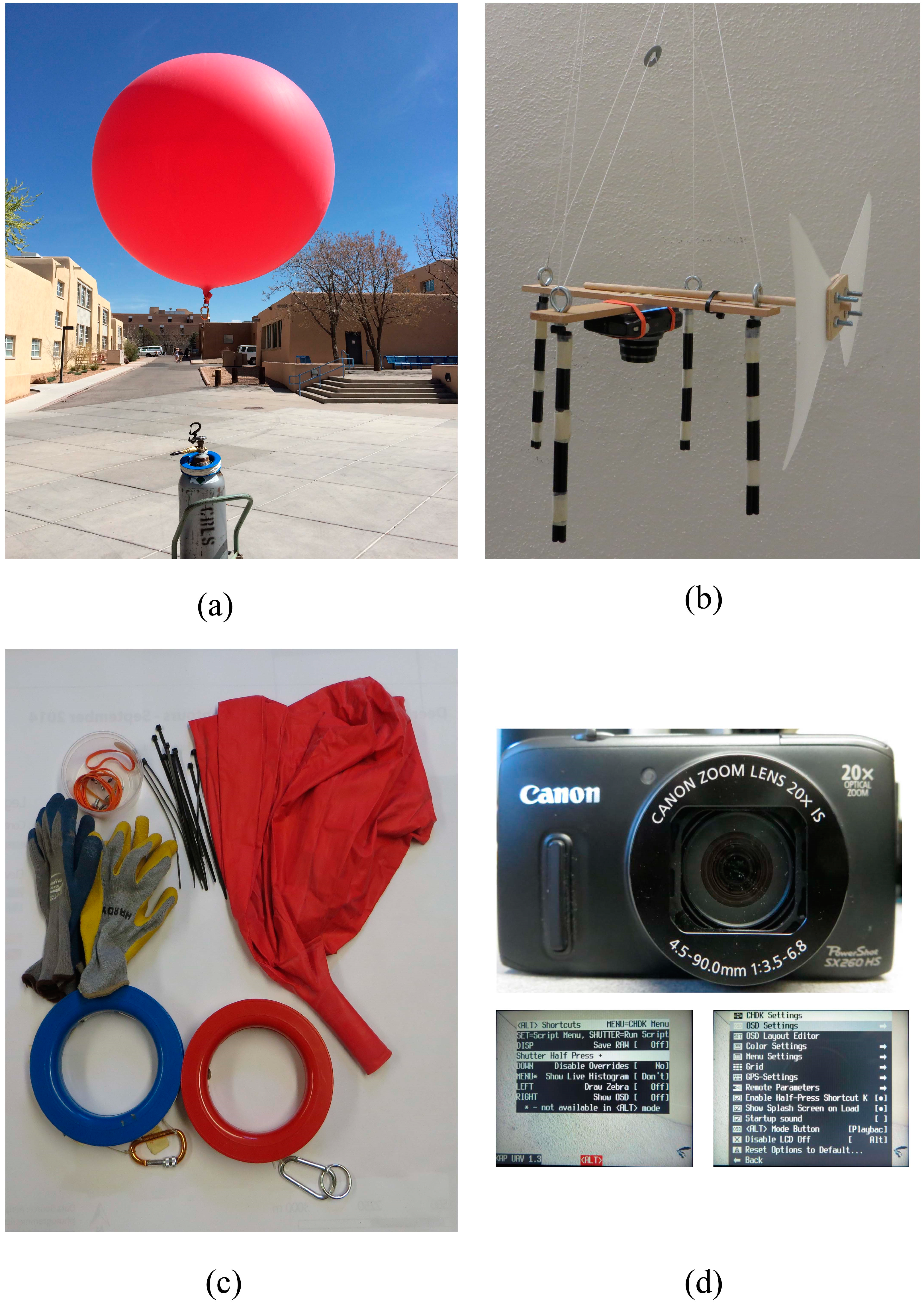
A low-altitude AGL and low-cost S-UAS was constructed to simulate the collection of HSR-AP from other untethered low altitude AGL S-UAS that are now common in the marketplace. This system includes a tethered helium weather balloon with custom-designed rigging based on the Picavet suspension system, as suggested by the Public Lab [43]. As mentioned in the previous section, a tethered helium weather balloon is permitted to fly in the United States of America as long as the flight meets the rules about location and altitude. The sensor affixed to the platform was an off-the-shelf small-format Canon SX260 HS digital camera. This camera has a 12-megapixel Complimentary Metal-Oxide Semiconductor (CMOS) detector array collecting in the visible blue, green, and red wavelength bands through Bayer array sampling and a built-in GPS unit. A firmware enhancement application known as the Canon Hack Development Kit (CHDK), was used to permit more control over the operation of the Canon SX260 HS camera, including shutter speed, shutter lag, aperture size, and intervalometer (Figure 1).

HSR-AP data were collected from 28 study sites (i.e., sections of roadway pavement surfaces) in Bernalillo County, New Mexico. Twenty-one sites were located on United States Highway 66, two sites were located on the campus of the University of New Mexico (UNM), and five sites were located on New Mexico Highway 333. All study site roadways run in a generally east-west direction. Approximately 300 overlapping HSR aerial images were acquired for each study site at about 5 m AGL to permit a nominal GSD of 0.002 m. At this AGL, the size of the ground area covered by each frame is approximately 8 × 6 m. Image acquisition was not controlled into flight lines, but was instead collected as a highly redundant block in a largely randomized pattern. However, the long side of each frame was approximately aligned perpendicular to the roadway while the short side of each frame was approximately parallel to the roadway. Crab angles were relatively stable along the roadways because balloon operators were standing along the shoulder of the roadways.

Ground control point (GCP) data were collected by a trained six-person surveying crew at each of the 28 sites. GCPs were identified using identifiable objects on the pavement surfaces, including sharp edges of cracking, intersections of cracking, and asphalt stains. GCPs were collected on the pavement surfaces using a survey grade CHC X900+ real-time kinematic (RTK) Global Navigation Satellite System (GNSS) in a base/rover configuration. Base stations were set up over National Geodetic Survey (NGS) benchmarks. Data were collected using the Carlson SurvCE software package and a WGS84 UTM Zone 13 North projection. When collecting the GCP coordinates, detailed photos of each GCP were acquired with the survey instrument in place. These detailed photos were used to facilitate the placement of GCPs on the acquired HSR aerial imagery. A total of 16 GCPs were collected for each site. The collected GCP coordinates were post-processed with the National Oceanic and Atmosphere Administration (NOAA) Online Positioning User Service (OPUS) and the ultimate root mean square (RMS) RTK accuracy achieved was 0.004 m + 1 ppm horizontally and 0.006 m + 1 ppm vertically.

A ground reference dataset of pavement surface conditions was collected by a trained two-person crew at each of the study sites. The crew performed manual measurements based on the standard evaluation protocols adopted by the HPMS Field Manual. Both inspectors assessed pavement surface distresses (rutting, alligator cracking, and transverse cracking) independently and the results were recorded as the average value of the two independent measurements. In accordance with the HPMS Field Manual, rutting depth was measured for only the rightmost driving lane for both inner and outer wheel paths at three locations along the wheel path within each site and then the depth was averaged for each wheel path. The HPMS Field Manual requires reporting the percent area of total alligator cracking to the nearest 5%. For transverse cracking, the HPMS Field Manual requires reporting an estimation of relative length in meters per kilometers (feet per mile).

2.2. Aerial Triangualtion

After excluding blurred and oblique HSR aerial images, between 120 and 300 overlapping aerial images were processed and assessed for each study site according to the protocols established by Zhang et al. [51]. As one of the most complex photogrammetric workflows, traditional AT is composed of many processes, which include image import, interior orientation, tie points determination, GCP measurements, bundle block adjustment, and quality control [52]. As in traditional AT, automated AT (or SfM) uses overlapping images acquired from multiple viewpoints [52]. However, automated AT differs from traditional AT by determining internal camera geometry using an in situ automated process and by triangulating camera position and orientation automatically without the need for a pre-defined set of visible GCPs at known 3D positions [53]. To do so, automated AT requires a high degree of overlap (ideally 75% for sidelap and 80% for forward overlap) to observe the full geometry of scene structure [46]. For this research, images were collected in a hyper redundant block pattern and the sidelap and forward overlap percentage meet or exceed the 75% and 80% requirements identified by Zhang et al. [46].

In recent years, many software packages have emerged to efficiently implement automated AT. The commercial software Agisoft Photoscan was selected as the tool of choice for this study as it permits minimal human intervention. Among the 16 GCPs, 10 were used to calibrate the automated AT process while the remaining six were reserved to evaluate the horizontal and vertical accuracy of the AT outputs, including orthophotos and DSMs.

For each of the 28 study sites, an in situ camera model was generated based on all of the input HSR aerial images. Therefore, the camera model is not identical across the sites. For each of the study sites, millions of tie points were automatically identified from the input of overlapping images to build a dense point cloud, and then a triangulation irregular network (TIN) mesh was generated based on the identified tie points. Lastly, a DSM was created based on the digital mesh and a mosaicked orthophoto was created based on input images to co-register with DSM.

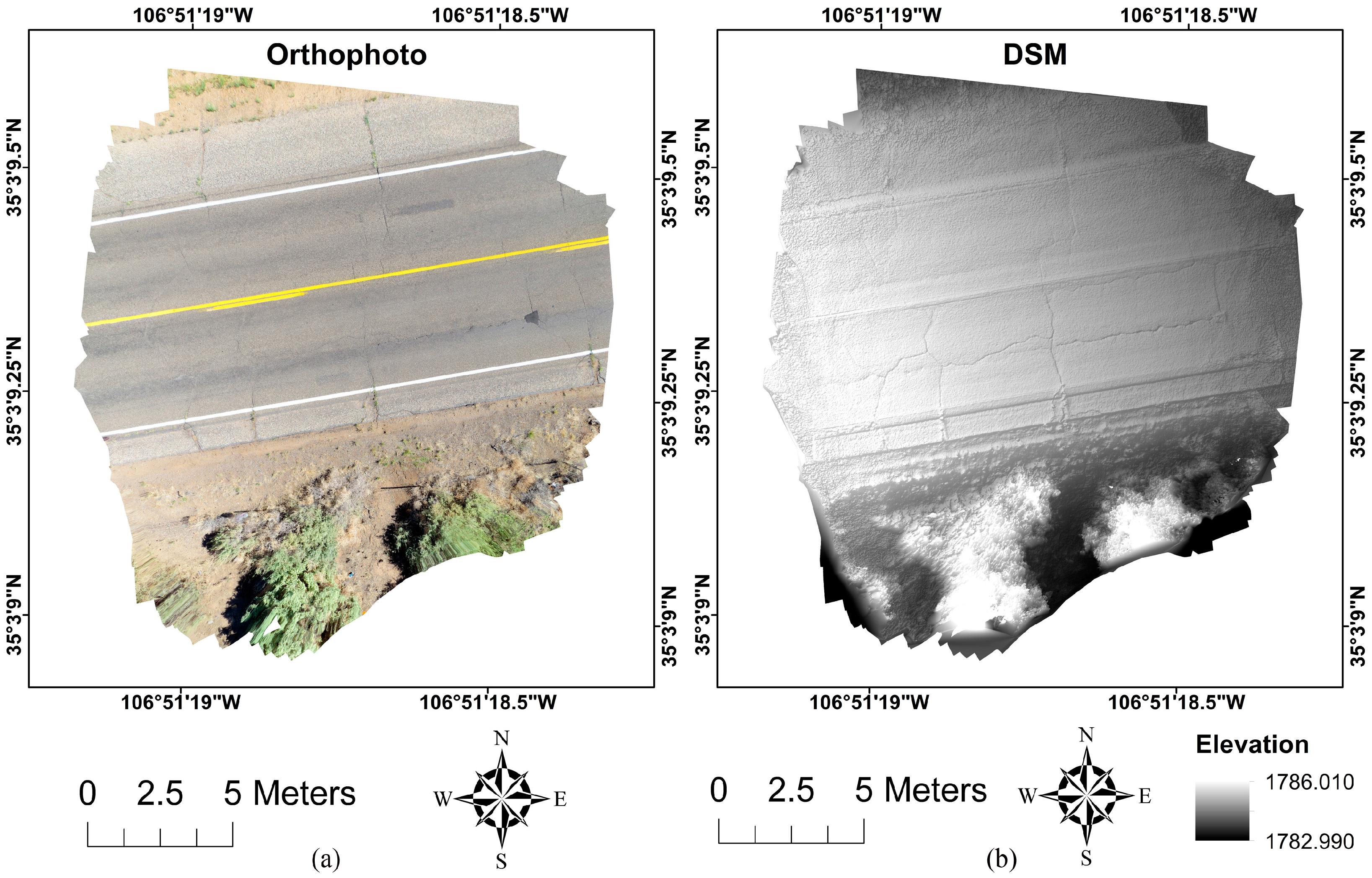
Once these processes were completed, orthophotos and the DSMs were exported as rasters in TIFF format at a spatial resolution of 0.003 m. Orthophotos and DSMs are generated in a single processing routine and are therefore tightly co-registered. An example of the orthophotos and DSM are showed in Figure 2. Orthophotos were used to assess the horizontal accuracy while DSMs were used to assess the vertical accuracy. Root-mean-squared-error (RMSE) was used to assess the accuracy [54], and the results show that the overall horizontal accuracy is 0.004 m while the overall vertical accuracy is 0.007 m. The number of overlapping images used and accuracy for each study site is reported in

Table 1. Accuracy Assessment Result (RMSE) for Each Study Site. RMSE refers to root-mean-squared-error.

Study Site	No. of Image Frames	Horizontal Accuracy (m)	Vertical Accuracy (m)
1	122	0.003	0.006
2	135	0.005	0.011
3	183	0.003	0.006
4	177	0.003	0.007
5	181	0.003	0.007
6	180	0.004	0.008
7	165	0.004	0.006
8	133	0.004	0.006
9	126	0.003	0.006
10	189	0.003	0.006
11	162	0.005	0.007
12	156	0.004	0.006
13	292	0.005	0.007
14	207	0.005	0.008
15	163	0.005	0.008
16	150	0.005	0.007
17	225	0.004	0.007
18	155	0.004	0.008
19	145	0.004	0.007
20	136	0.003	0.005
21	168	0.004	0.006
22	130	0.003	0.006
23	105	0.003	0.006
24	103	0.004	0.005
25	109	0.004	0.006
26	155	0.004	0.007
27	112	0.003	0.006
28	115	0.003	0.006
Mean	157	0.004	0.007

. More details regarding the accuracy assessment can be found in the study performed by Zhang et al. [51].

2.3. Rutting Depth Measurement

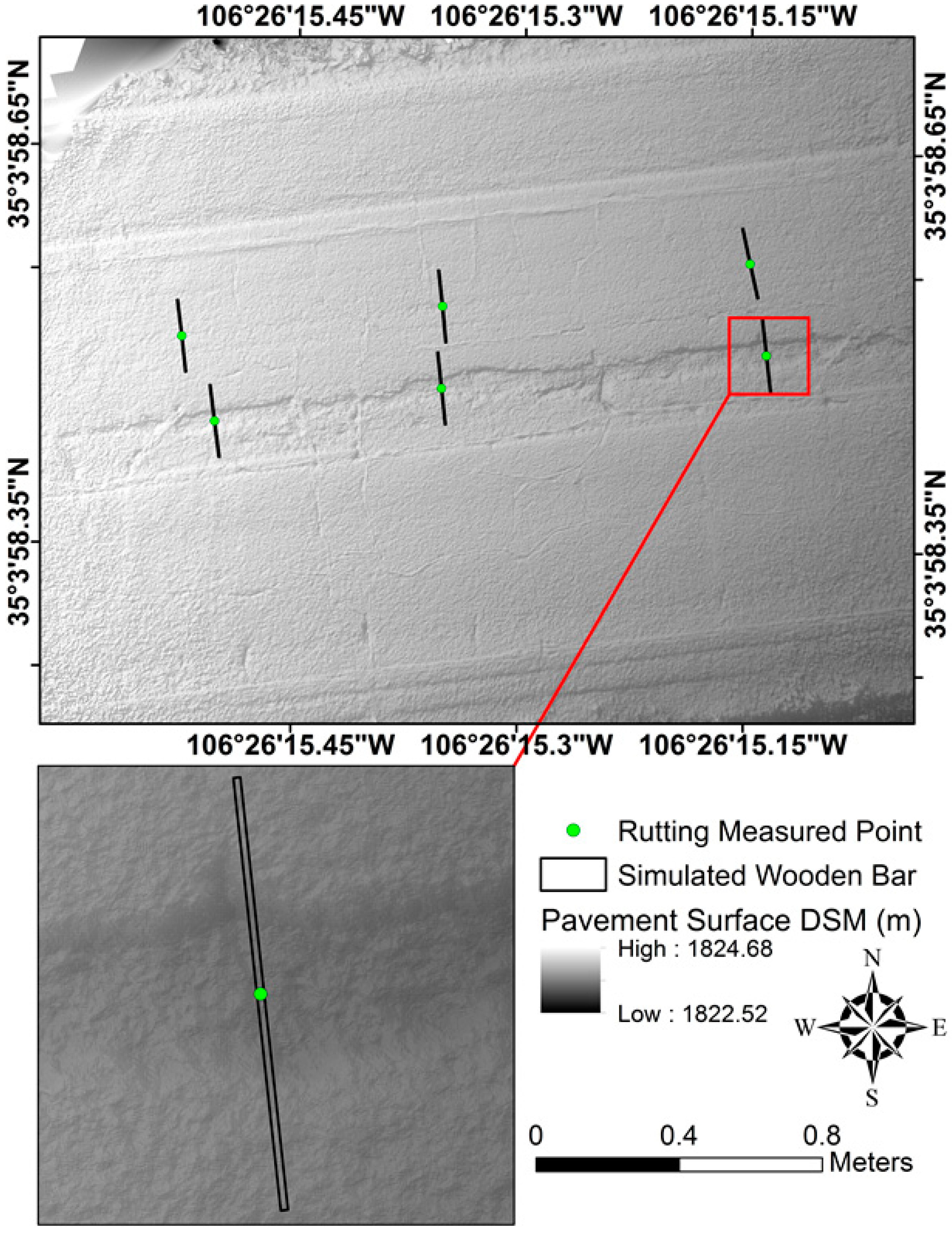
Rutting is an unrecoverable longitudinal surface depression in both inner and outer wheel paths [50]. In ground-based manual measurement, rutting depth was measured with a wooden bar and a measuring tape. The wooden bar was used as a reference line between the two highest points of the rut and the measuring tape was used to measure the distance from the lowest point on the pavement surface perpendicularly to the point at the bottom of the wooden bar that is perpendicular to the lowest point. The actual measured points in the field are the lowest points as visually determined by inspectors. The minimum scale of the measuring tape used for manual evaluation was 0.001 m. The length and width of the wooden bar is 1.22 m (48-inch) and 0.02 m (0.8-inch).

DSMs (reconstructed 3D pavement surface) were used to measure rutting depths using a digital process designed to simulate the ground-based manual measurement. Points and polygons were created on DSMs to simulate the locations of the actual measured points and wooden bars. The actual measured points in the field and the locations of the wooden bars are shown in Figure 3. With the actual measured point (as photographed in the field) as the center, two polygons (one on either side of the filed measured point) with a size of 0.61 m by 0.02 m were created to simulate the location of the wooden bar.

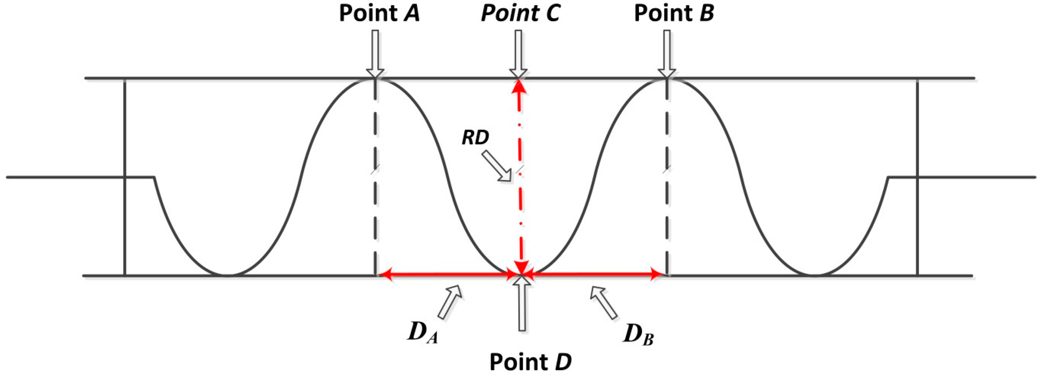
Unlike ground-based manual measurement, it is not possible to directly identify the highest point at the bottom of the wooden bar. Therefore, the following method was used to identify the highest and lowest points of rutting. Using the polygon as the boundary, the DSM pixels within the boundary were extracted and reclassified to find the highest point on both sides of the actual field measured points. If there were multiple pixels having the same highest value, the one closer to the actual measured point in the field was used. Then, as shown in Figure 4, we considered the two highest points within the two polygons as Point A and Point B, while the two measured points as Point C and Point D. The distance from Point C to Point D is the rutting depth. Points A, B, and C will have the same height if the heights of Points A and B are equal. However, under most circumstances the heights of Points A and B are different. Therefore, a weighted average method was used to calculate the height of Point C:

$$H_C= \frac{H_A*D_A+H_B*D_B}{D_A+D_B}$$

(1)

$$RD=H_C-H_D$$

(2)

where H represents the height of a given point, and therefore H_A represents the height of Point A, and H_B represents the height of Point B. D_A represents the horizontal distance from Point A to Point D, while D_B represents the horizontal distance from Point B to Point D. RD represents the rutting depth. H_A and H_B were determined from the DSMs, while D_A and D_B were determined from the orthophotos.

2.4. Alligator Cracking Measurement

Alligator cracking is interconnected cracks resembling check wire or alligator skins [50]. Longitudinal cracking (cracks that are parallel to the pavement’s centerline) should also be included as alligator cracking [49]. According to the HPMS Field Manual, alligator cracking should be reported as the percentage of the total evaluated area to the nearest 5% at a minimum. In manual evaluation, inspectors measure the cumulative length of alligator cracking and mark the location of occurrence in one or two wheel paths. For example, typically the width of the driving lane is 3.66 m (12 ft), and therefore, for a 100 m (328 ft) section, the total area is 366 m² (3940 ft²). If alligator cracking exists for both wheel paths, and for each wheel path the total length of the measured alligator cracking is 15 m (49 ft) while the width is 0.5 m (1.64 ft), the total area of the measured alligator cracking is 15 m² (15 × 0.5 × 2 = 15). There the total area percentage should be 5 percent (15/366 × 100 = 4.09%, which should be rounded up to the nearest 5 percent, which is 5%).

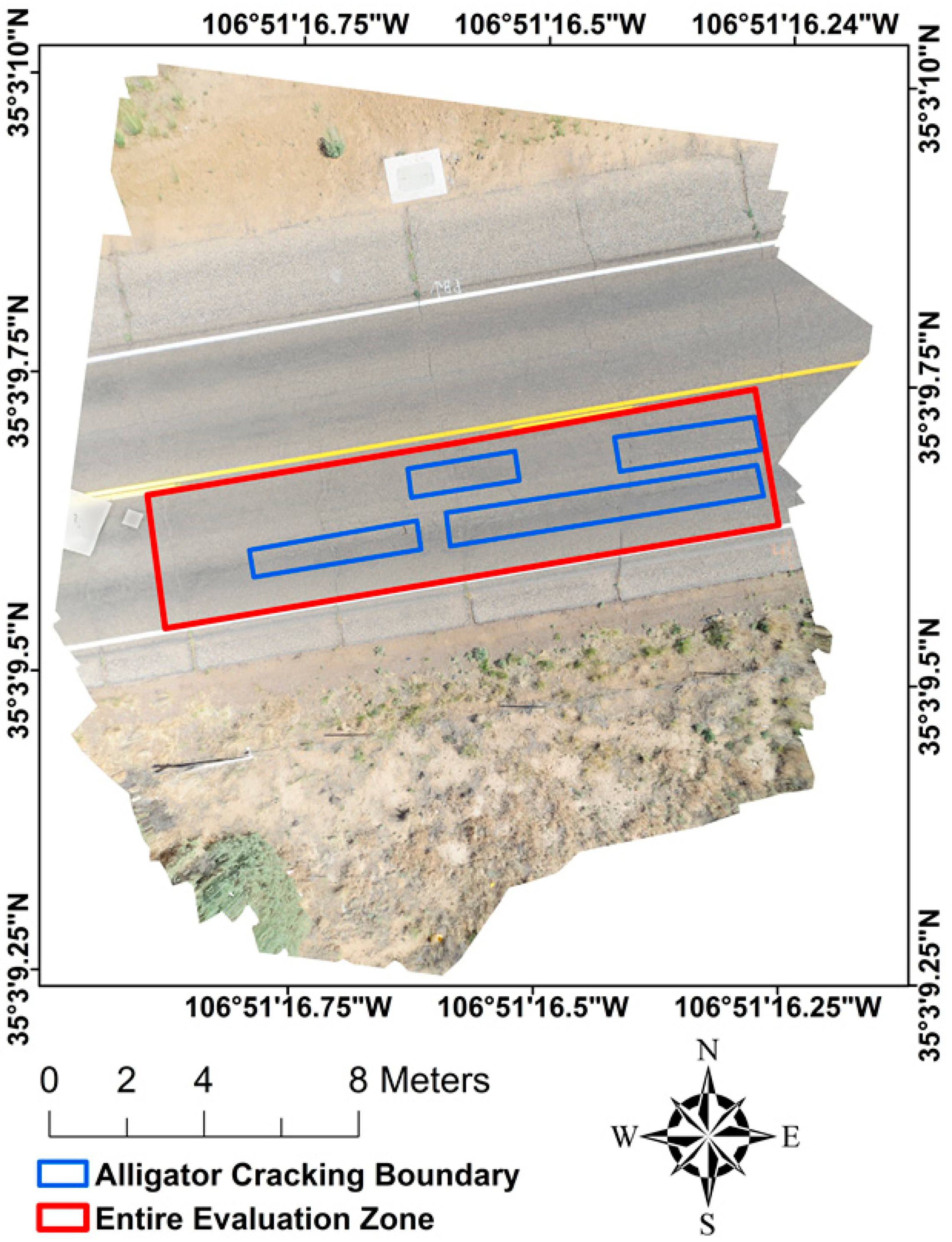
In order to simulate the alligator cracking measurement prescribed by the HPMS Field Manual, orthophotos were visually analyzed to locate alligator cracks and then mark them with on-screen digitization in GIS software. Polygons were digitized to represent both the entire evaluated pavement section and the sections that alligator cracking occurred. The polygon defining the entire evaluated pavement section was used to calculate the total evaluated area, while the polygons defining alligator cracking were used to calculate the total area of alligator cracking. The area percentage of alligator cracking was then calculated by comparing the areas of the two sets of polygons. The use of polygons to determine area percentage of alligator cracking is shown in Figure 5. It should be noted that both actual area percentage and rounded area percentage were calculated for each site, but only rounded area percentage was used for comparison to ground-based manual measurements.

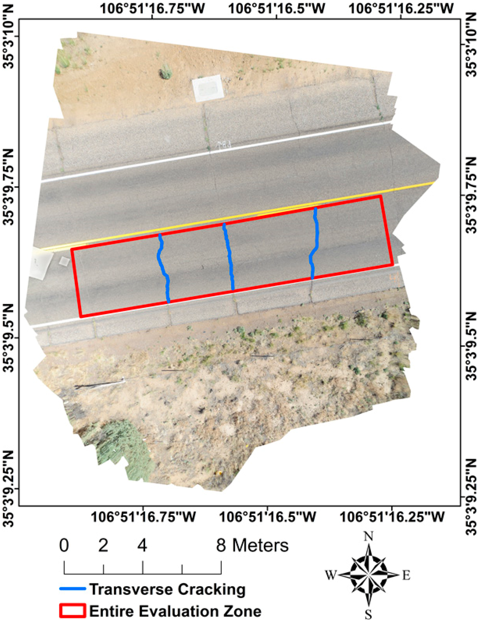
2.5. Transverse Cracking Measurement

Transverse cracking are cracks that are perpendicular to the pavement’s centerline [50]. According to the HPMS Field Manual, field inspectors should measure the length of each transverse crack that extends at least half of the lane width (1.83 m [6 ft] or longer cracks) to calculate the total length of transverse cracking. The total length of transverse cracking will be normalized by the total length of the evaluated pavement section, and therefore, the final results will be delivered in the format of meter per kilometer (or feet per mile).

In order to simulate the transverse cracking measurement prescribed by the HPMS Field Manual, orthophotos were visually analyzed and any transverse cracks longer than 1.83 m (6 feet) were identified and digitized in GIS software as polylines to facilitate the calculation of total length of transverse cracking (Figure 6). The same polygon created for the alligator cracking measurement representing the entire evaluated pavement section was used to measure the total length of the evaluated pavement section.

2.6. Measurement Results Comparision

For each study site, rutting depth (for both wheel paths), alligator cracking area percentage, and transverse cracking length measured from the DSMs and orthophotos were compared with ground-based manual measurement results to examine the utility of using HSR-AP derived products to detect and assess detailed pavement surface distresses. In order to select the most appropriate statistical test, the sample size of each set of measurements was examined. Most statistical researchers and scientists accept that non-parametric statistical tests should be employed if the sample size is less than 30 [55,56,57,58], even if sample values are normally distributed. The examination revealed that the sample size for each set of measurements was 28, and therefore, non-parametric statistical tests were used to compare ground-based measurements with HSR-AP derived products based measurements.

Measurement comparisons were performed as a paired group and unpaired group. Paired group tests are more appropriate if two groups of measurements are dependent (i.e., repeated measurements for the same subject but at two different times). Unpaired group tests are more appropriate if two groups of measurements are independent (i.e., measurement for one sample in Group A has no bearing on the measurement for one sample in Group B). The relationship between ground-based manual measurements and HSR-AP derived products measurements can be interpreted in both a dependent way and an independent way. In the dependent way, repeated measurements of a specific distress at a study site were performed on the ground and from HSR-AP derived products at two different times, and therefore, they are dependent. In the independent way, the ground-based measurement of a specific distress at a study site has no bearing on the HSR-AP derived product based measurement of a specific distress at the same study site since they are measured from two different data sources. Since the relationship can be interpreted in both ways, to err on the side of caution, this research used both paired group and unpaired group statistical tests to examine if the detailed pavement surface distress rates measured from HSR-AP derived products and distress rates manually measured on the ground are statistically different.

In the paired group comparisons, repeated measurements (i.e., ground-based measurement and HSR-AP derived products based measurement) of a specific distress (e.g., alligator cracking) for a specific study site (e.g., site 20) constitute a pair, and the purpose of this comparison is to examine whether the median difference between the two sets of paired measurements is zero. Nonparametric Wilcoxon Signed Rank test [59], which does not assume normality in the data, was used in this study as a robust alternative to parametric Student’s t-test.

In the unpaired group comparisons, two sets of measurements (i.e., the ground-based measurement and the HSR-AP derived products based measurement) of a specific distress constitute two independent groups, and the purpose of this comparison is to examine whether two independent groups of samples exhibit the same distribution pattern (i.e., shape and spread) or have differences in medians. Nonparametric Mann-Whitney U test [60], also known as Wilcoxon Rank-Sum test, which also does not assume normality in the data, was used to detect differences in shape and spread as well as differences in medians.

3. Results

For rutting depth, the ground-based and DSM-based measurements are summarized in

Table 2. Rutting Depth Measurements for Inner and Outer Wheel Path (in m).

Site ID	Inner Wheel Path		Outer Wheel Path
	Ground Depth	DSM Depth	Ground Depth	DSM Depth
1	0.021	0.024	0.006	0.009
2	0.012	0.020	0.009	0.017
3	0.015	0.016	0.007	0.007
4	0.017	0.017	0.008	0.013
5	0.022	0.019	0.018	0.015
6	0.019	0.016	0.021	0.017
7	0.017	0.022	0.018	0.023
8	0.022	0.018	0.018	0.017
9	0.013	0.013	0.016	0.018
10	0.008	0.010	0.015	0.016
11	0.020	0.016	0.024	0.021
12	0.023	0.019	0.014	0.014
13	0.017	0.018	0.010	0.013
14	0.010	0.015	0.007	0.009
15	0.010	0.014	0.011	0.012
16	0.017	0.014	0.018	0.012
17	0.008	0.013	0.007	0.011
18	0.014	0.014	0.015	0.011
19	0.007	0.010	0.011	0.011
20	0.016	0.013	0.007	0.009
21	0.015	0.011	0.017	0.014
22	0.010	0.007	0.009	0.006
23	0.010	0.005	0.006	0.008
24	0.003	0.006	0.010	0.005
25	0.003	0.005	0.007	0.006
26	0.003	0.007	0.003	0.007
27	0.002	0.004	0.004	0.004
28	0.024	0.031	0.025	0.033

. It should be noted that the results are organized by inner and outer wheel paths for each study site.

Table 3. Alligator Cracking Area Percentage and Transverse Cracking Length Measurements.

Site ID	Alligator Cracking Area Percentage (%)		Transverse Cracking Length (m/km)
	Ground Measure	Orthophoto Measure	Ground Measure	Orthophoto Measure
1	10	10	638	660
2	5	5	728	783
3	5	5	606	589
4	15	15	1326	1290
5	5	10	1395	1410
6	25	20	1032	1064
7	20	25	774	766
8	20	20	1113	1098
9	15	10	1136	1148
10	25	25	653	632
11	20	20	814	771
12	35	35	1141	1121
13	30	30	1145	1212
14	25	25	1186	1136
15	20	25	859	905
16	45	45	1219	1256
17	25	25	649	682
18	30	30	839	815
19	25	25	1135	1102
20	25	25	958	978
21	15	15	665	683
22	5	5	264	280
23	5	5	369	359
24	5	10	175	202
25	10	10	248	284
26	10	10	263	290
27	0	0	0	0
28	35	35	534	500

summarizes the ground-based and orthophoto-based measurements for alligator cracking area percentage and transverse cracking length.

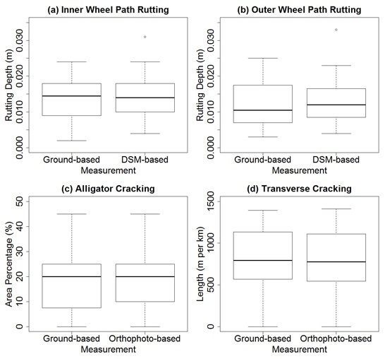
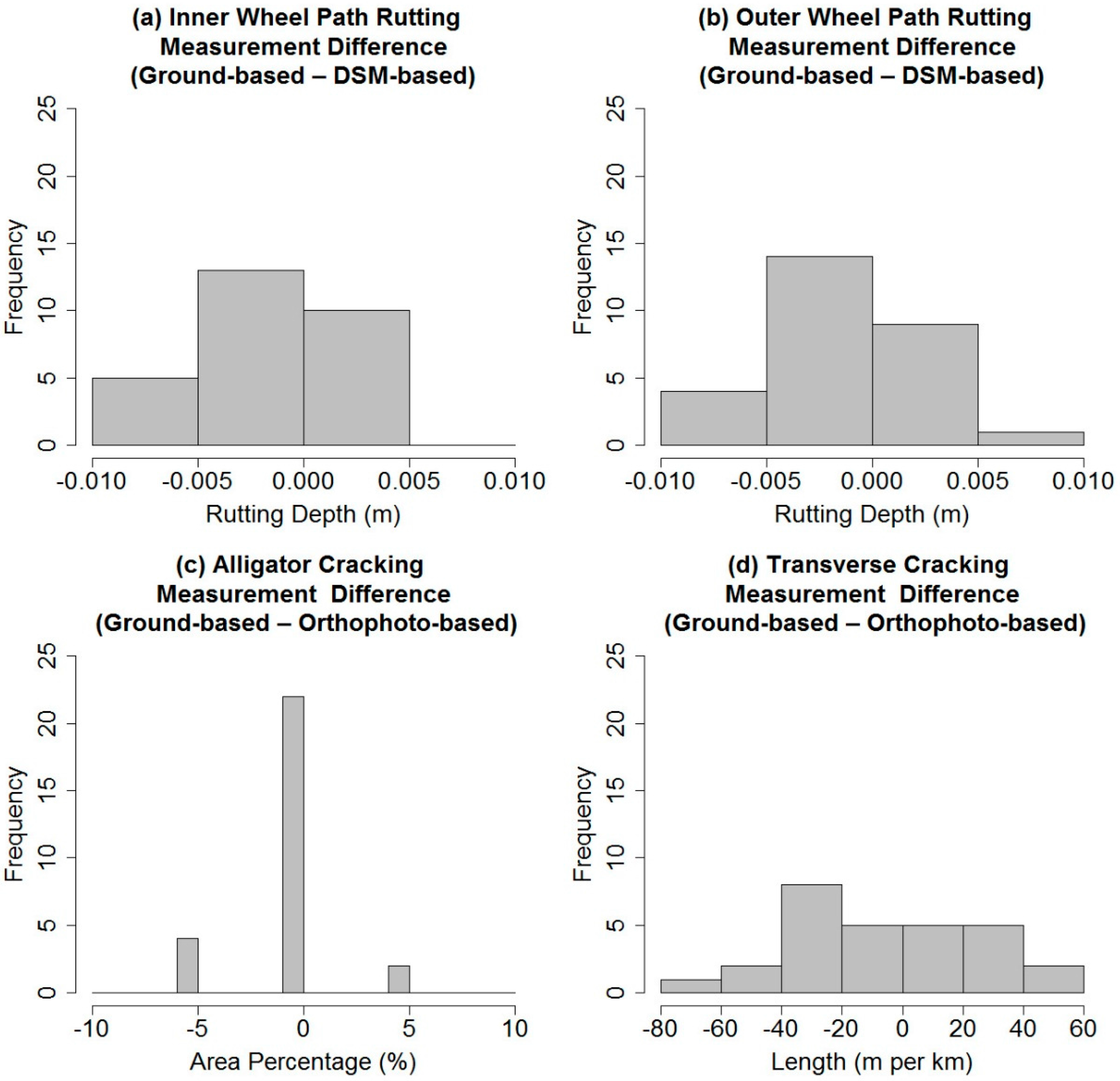
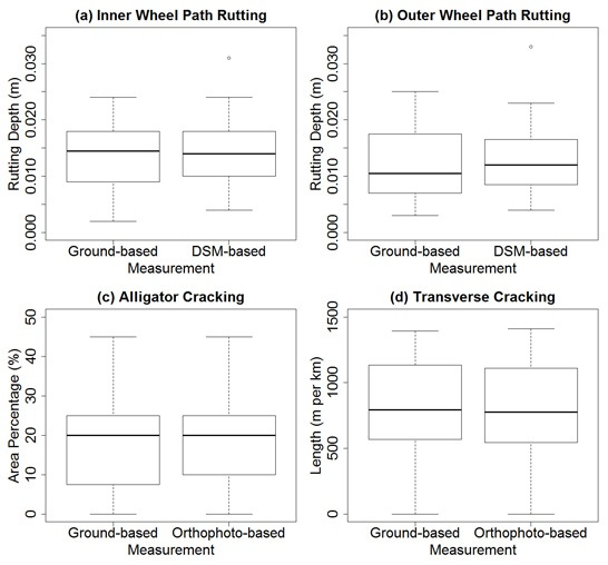
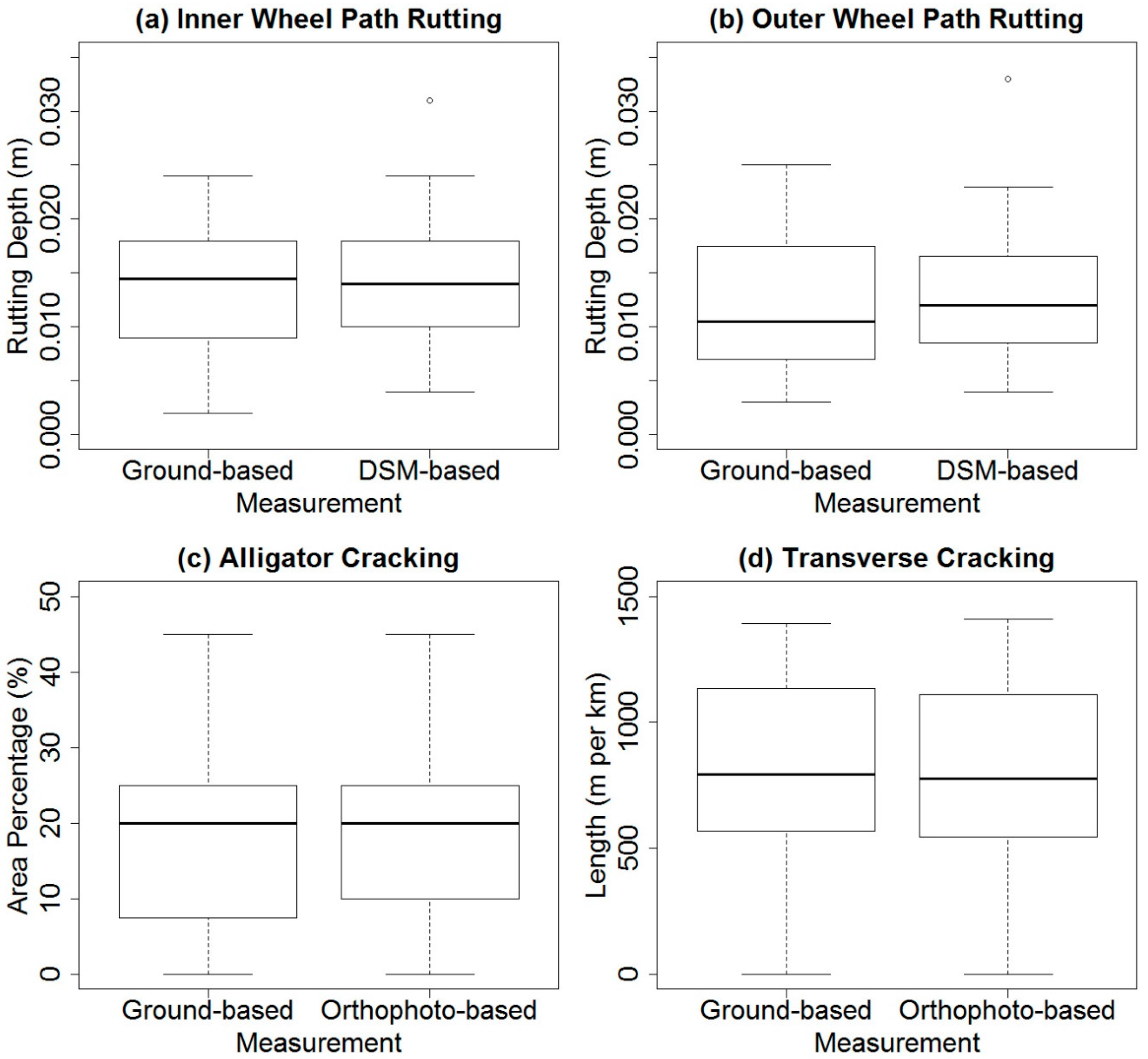
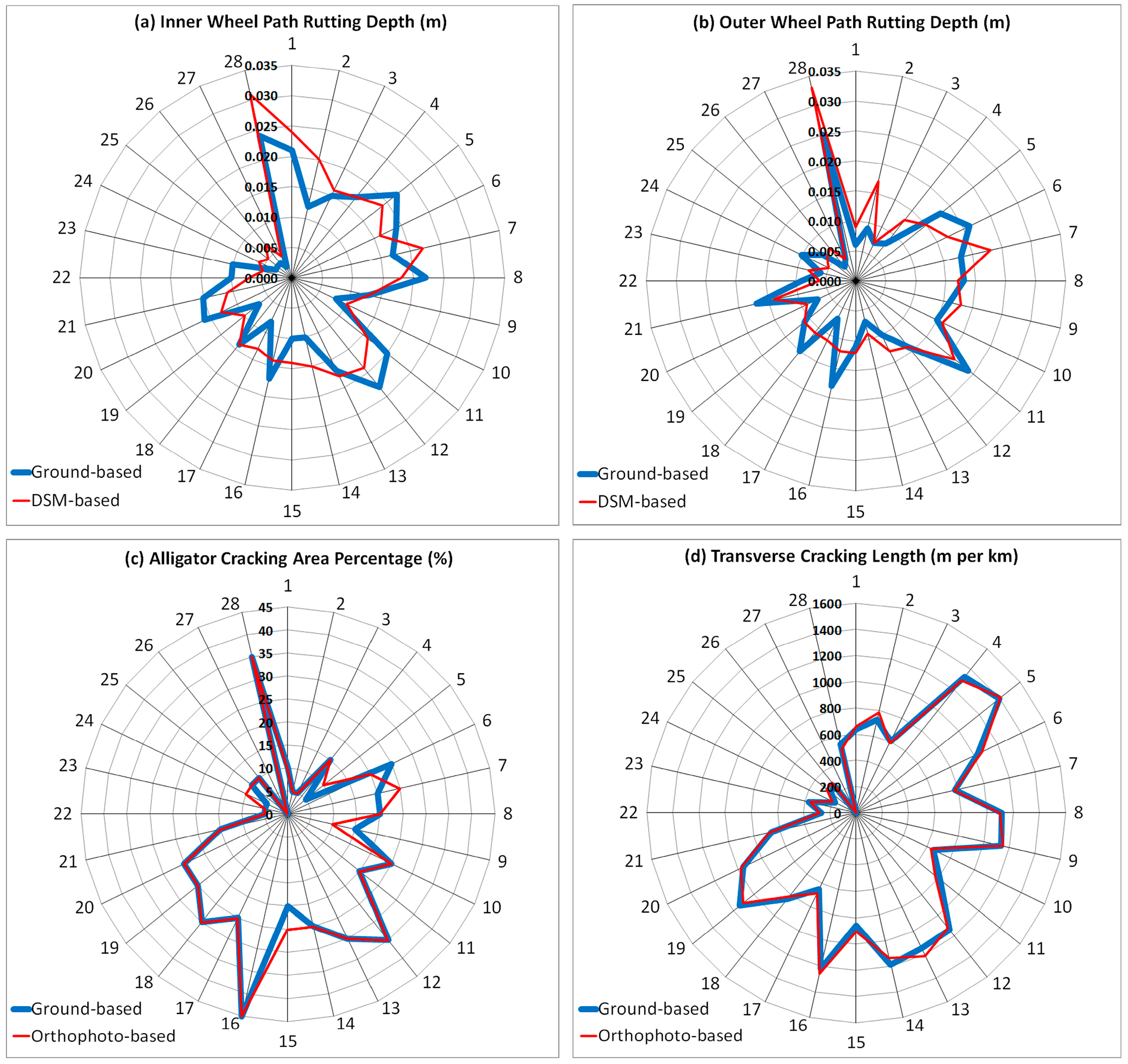
The box plots, histogram plots, and radar plots displaying each set of measurements were visually examined and are shown in Figure 7, Figure 8 and Figure 9. Box plots revealed that only DSM-based rutting measurement showed evidence of outliers (dots found above the whiskers). However, box plots did not show a substantial difference in the medians between ground-based measurements and HSR-AP derived products based measurements. There also did not appear to be a substantial difference in the box sizes. Histogram plots provide a visual presentation of the frequency distribution of each distress’ measurement differences (residuals). Measurement difference was defined as the difference between ground-based measurement and HSR-AP derived products based measurement. The plots did not show a substantial difference in the two sets of measurements for each distress. Most of the residuals were distributed around the value of zero. Radar plots provide another visual presentation of the measured distress rates for each study site. The plots did not reveal a substantial difference in the shape and spread of distribution between the two sets of measurements for each distress.

Continuing with visual analysis, formal statistical tests were performed. The Wilcoxon Signed Rank test was performed to compare the measurement results of each type of distress at the paired group level. For rutting depth, the test was performed for both the inner wheel path and outer wheel path. For each comparison test, the null hypothesis is that the median difference between each pair of measurements is zero. Test results are summarized in

Table 4. Wilcoxon Signed Rank Test Results for Each Distress.

Test ID	Distress	Null Hypothesis	p-Value
1	Inner Wheel Path Rutting Depth	The median difference between the two paired measurements (ground-based measurement vs. DSM-based measurement) is zero	0.424
2	Outer Wheel Path Rutting Depth	The median difference between two paired measurements (ground-based measurement vs. DSM-based measurement) is zero	0.541
3	Alligator Cracking Area Percentage	The median difference between two paired measurements (ground-based measurement vs. orthophoto-based measurement) is zero	0.688
4	Transverse Cracking Length	The median difference between two paired measurements (ground-based measurement vs. orthophoto-based measurement) is zero	0.701

. For each pair of measurements, p-values are greater than 0.05, and therefore the null hypothesis should be accepted; thereby indicating that for each distress the median difference between the paired ground-based measurement and HSR-AP derived products based measurement is zero at a 95% confidence interval. In other words, for rutting, alligator cracking, and transverse cracking, ground-based measurements and HSR-AP derived products based measurements are not statistically different at a 0.05 significance level.

The Mann-Whitney U test was performed to compare the measurement results of each distress unpaired, as a group. For rutting depth, the test was again performed for both the inner wheel path and outer wheel path. Although the Mann-Whitney U test does not require normally distributed data, it does not mean that it is assumption free. For the Mann-Whitney U test, data from each population must be an independent random sample, and the population must have equal variances. For non-normally distributed data, the Levene’s test and Barlett’s test are usually adopted to determine variance equability.

For the Levene’s test and the Barlett’s test, the null hypothesis is that the population variances are equal. Test results are summarized in

Table 5. Levene’s Test and Bartlett’s Test Results.

Distress	Comparison	Null Hypothesis	Variance Test p-Value
			Levene’s Test	Bartlett’s Test
Inner Wheel Path Rutting Depth	Ground-based Measure vs. DSM-based Measure	Population variances are equal	0.481	0.832
Outer Wheel Path Rutting Depth	Ground-based Measure vs. DSM-based Measure	Population variances are equal	0.546	0.866
Alligator Cracking Area Percentage	Ground-based Measure vs. DSM-based Measure	Population variances are equal	0.987	0.929
Transverse Cracking Length	Ground-based Measure vs. DSM-based Measure	Population variances are equal	0.946	0.962

. For each comparison, the p-value is greater than 0.05, and therefore the null hypothesis should be accepted; thereby indicating that the population variances for each pair of comparisons are equal at a 95% confidence interval. Therefore, the Mann-Whitney U test is appropriate for all metrics.

For each of the Mann-Whitney U tests, the null hypothesis is that there is no difference in the distribution (shape and spread) of ground-based measurement and HSR-AP derived products based measurement. For all tests, the null hypothesis was retained, meaning that there is no significant difference in the distribution pattern (

Table 6. Mann-Whitney U Test for Each Distress.

Test ID	Distress	Null Hypothesis	p-Value
1	Inner Wheel Path Rutting Depth	The distribution pattern (shape and spread) of measurement values for ground-based measure vs. DSM-based measure is the same	0.850
2	Outer Wheel Path Rutting Depth	The distribution pattern (shape and spread) of measurement values for ground-based measure vs. DSM-based measure is the same	0.786
3	Alligator Cracking Area Percentage	The distribution pattern (shape and spread) of measurement values for ground-based measure vs. orthophoto-based measure is the same	0.855
4	Transverse Cracking Length	The distribution pattern (shape and spread) of measurement values for ground-based measure vs. orthophoto-based measure is the same	0.948

) at a 95% confidence interval.

4. Discussion

Formal statistical test results revealed that there is no evidence showing that detailed pavement surface distress (i.e., rutting, alligator cracking, and transverse cracking) rates measured from HSR-AP derived products and distress rates manually measured on the ground using standard protocols are statistically different at a 0.05 significance level. Visual comparison of the results supports this finding. Ultimately, these results show that orthophotos and DSMs generated from HSR-AP acquired from S-UAS can be effectively used to characterize detailed pavement surface distress that is comparable to ground-based manual measurement.

It should be noted that current manual evaluation methods operationally used by transportation management agencies rely on only visual observation to estimate distress rates (e.g., estimate the length of the cracks), which is highly subjective [21]. However, inspectors of this research physically measured the distress rates to collect ground reference data, which is objective. When using the on-screen analysis and digitization to detect and assess distress, the inspectors did not digitize a crack unless it exists and the inspectors were able to identify it, which is also objective. Given the horizontal and vertical accuracy (RMSE = 4 mm and 7 mm, respectively) of the orthophotos and DSMs, the discrepancy between the ground-based manual measurement method and the HSR-AP method could be from either method. This is because distress measurements made by inspectors involves random errors which cannot be avoided [61,62].

Further investigation of the measurements for each type of distress revealed a more detailed pattern. For the inner and outer wheel path rutting depth, DSM-based measurements are generally higher than ground-based measurements, with 15 sites showing higher DSM-based rutting depth and only ten sites exhibiting higher ground-based rutting depth. The measured vertical accuracy (RMSE = 7 mm) of the DSMs can be interpreted as an indication that much of the discrepancy between the two methods is likely a product of variability in the reconstructed DSMs. This also indicates that DSM-based measurement has a tendency to overestimate rutting depth. Increasing the vertical accuracy of DSMs may be able to reduce the variability in the reconstructed DSMs, and ultimately reduce the variability in rutting depth measurement.

For alligator cracking area percentage, 22 sites have equal orthophoto-based measurements and ground-based measurements. For transverse cracking, the percent difference between orthophoto-based measurements and ground-based measurements for 20 sites are less than 5%. The measured horizontal accuracy (RMSE = 4 mm) of the orthophotos can be interpreted as an indication that much of the discrepancy between the two methods is likely a product of variability in the field measurements. Field measurement is prone to disturbances originated from traffic, weather conditions, physical conditions, and so on. However, on-screen digitization is not affected by these factors.

Formal statistical test results and visual comparison of results also reveal that discrepancies in the vertical (i.e., rutting) are higher than in the horizontal (i.e., alligator cracking and transverse cracking). However, these results may not indicate that the proposed method works more effectively for characterizing horizontal pavement surface distresses such as cracking. This is because cracking measurements were rounded (for alligator cracking) or normalized (for transverse cracking), which would increase apparent accuracy. In contrast, rutting measurement in the field or on DSMs was error prone, which would decrease apparent accuracy.

Although the novel aspect of this research lies in evaluating whether HSR-AP acquired from S-UAS can be used to characterize detailed pavement surface distress conditions, the remote sensing techniques and methods (e.g., S-UAS based hyper-spatial resolution imaging, SfM, and digitization) associated with this research are readily deployable for detailed pavement surface condition assessment once restrictions on S-UAS operations are lifted. SfM enabled AT to leverage graphic processing units to permit the generation of tightly co-registered orthophotos and DSMs from large HSR aerial image sets. Collectively, these techniques enabled the 3D characterization of pavement surfaces at unprecedented millimeter scales. In a broader context, the proposed method can be used for myriad other infrastructure condition inspection tasks. These results can be replicated by researchers or practitioners from the infrastructure management and asset management communities to assess whether HSR-AP acquired from S-UAS can be used characterize their managed infrastructure or assets such as oil and gas pipelines, bridges, and dams.

Although detailed pavement surface distress conditions are detected and assessed through manual digitizing, it is actually less labor-intensive, less expensive, and more accurate when compared with operationally used ground-based manual observation. The physical and financial requirements for digitization are less than for ground-based manual observation. This is because inspectors are not required to drive to the evaluation destination and walk or drive along the roadways to perform inspection. When inspectors are conducting ground-based physical measurement, at least three people are required because one of them is designated as the safety spotter (inspectors do not have the authority to stop the traffic) and two of them perform the physical measurements. The time for the three-people crew to complete an evaluation for a pavement section with a size of 8 m by 6 m is approximately 20 min. However, evaluating the same pavement section with HSR-AP derived products will only need one inspector for approximately 10 min.

Undeniably, there are costs associated with acquiring HSR-AP from S-UAS, but the cost of using S-UAS acquired aerial data has been substantially reduced in recent years [42]. In addition, the cost can be reduced by collaborating with various government agencies such as the U.S. Geological Survey (USGS), U.S. Department of Agriculture (USDA), and U.S. Department of Homeland Security (USDHS) because these agencies also need HSR aerial imagery data for their managerial activities. Long-term archived HSR aerial imagery records also provide transportation management agencies with the capability to identify spatial and temporal patterns of pavement surface distress conditions from a primary record. It should also be noted that high costs cannot prevent a method from deployment if it has other advantages. For example, New Mexico Department of Transportation (NMDOT) had been using visual observation methods to annually evaluate their 12,500 miles of roadways for many years at an annual cost of approximately $720,000. However, recently NMDOT adopted survey vehicle-based automated evaluation methods and the annual cost jumped to approximately $2,100,000 [63].

More importantly, manual digitization is much more accurate than currently adopted manual observation methods which are based on only subjective judgement (no physical measurement). Formal statistical test results reveal that HSR-AP derived products based measurements are comparable to ground-based measurements. For this research, inspectors performed physical measurements to ensure consistent and reliable measures of distress on which to evaluate the efficacy of HSR-AP derived measures.

Even if the proposed methods are readily deployable, the next logical step is automating the extraction of pavement surface distress metrics given the data quantities involved [42]. Automation will reduce the cost of scaled operational deployment as the U.S. Federal Aviation Administration (FAA) establishes regulations and clears restrictions for S-UAS work in the near future. One potential approach to automate the extraction of alligator cracking and transverse cracking is geographic object-based image analysis (GEOBIA) methods [64]. One potential approach to automate the extraction of rutting depth is having digitized wheel path polygons stored in a GIS database and then routinely monitoring their height change by comparing DSMs acquired at different times (e.g., yearly). Nevertheless, significant algorithm development will be required for both potential approaches, especially for cracking detection and assessment. It might be comparatively easy to identify transverse cracking, but the path to computational rules defining alligator cracking is less clear. For example, according to the HPMS manual, longitudinal cracking should be considered alligator cracking if it occurs in inner or outer wheel paths.

To summarize, S-UAS based hyper-spatial resolution imaging and AT techniques can be used to provide detailed and reliable primary observations suitable for characterizing detailed pavement surface distress conditions, which lays the foundation for the future application of these techniques for automated detection and assessment of detailed pavement surface distress conditions. Operationally HSR-AP based pavement surface evaluation could be implemented as a service internally by transportation agencies or implemented through consulting firms. Eventually the extraction of distress metrics from HSR-AP should be automated to enable cost effective scaling of S-UAS based asset management, requiring end users (i.e., federal, state, or local transportation management agencies) only to design a flight plan and select the distresses to be evaluated, with all other processes being automated.

5. Conclusions

This research evaluated whether HSR-AP acquired from S-UAS can be used to characterize detailed roadway pavement surface distress conditions. Research results indicate that using HSR-AP acquired from S-UAS as input, AT can be used to generate millimeter scale orthophotos and DSMs and these products can be effectively used to characterize detailed pavement surface distresses comparable to ground-based manual measurement. This finding lays the foundation for future research into automated pavement surface distress detection and assessment by demonstrating that HSR-AP has the capability to provide accurate and reliable information to characterize detailed pavement surface distress conditions; automation is the logical next step. In recent years, many other sensors such as thermal infrared (IR) and LiDAR are becoming commercially available in miniaturized forms suitable for operation on S-UAS. Many of these sensors, while more expensive per sensor, have the potential to improve detailed pavement surface distress evaluation. In the near term, the proposed digitization method could be used to measure pavement surface conditions in situations where field inspectors cannot evaluate without considerable labor costs (e.g., sections in remote areas) or where survey vehicles cannot gain access; however, in the long term, the proposed method is capable of completely replacing field pavement surface distress evaluation due to its high accuracy, potential for full automation, and the potential to dramatically reduce long-term cost.