Abstract
To alleviate the severe rocky desertification and improve the ecological conditions in Southwest China, the national and local Chinese governments have implemented a series of Ecological Restoration Projects since the late 1990s. In this context, remote sensing can be a valuable tool for conservation management by monitoring vegetation dynamics, projecting the persistence of vegetation trends and identifying areas of interest for upcoming restoration measures. In this study, we use MODIS satellite time series (2001–2013) and the Hurst exponent to classify the study area (Guizhou and Guangxi Provinces) according to the persistence of future vegetation trends (positive, anti-persistent positive, negative, anti-persistent negative, stable or uncertain). The persistence of trends is interrelated with terrain conditions (elevation and slope angle) and results in an index providing information on the restoration prospects and associated uncertainty of different terrain classes found in the study area. The results show that 69% of the observed trends are persistent beyond 2013, with 57% being stable, 10% positive, 5% anti-persistent positive, 3% negative, 1% anti-persistent negative and 24% uncertain. Most negative development is found in areas of high anthropogenic influence (low elevation and slope), as compared to areas of rough terrain. We further show that the uncertainty increases with the elevation and slope angle, and areas characterized by both high elevation and slope angle need special attention to prevent degradation. Whereas areas with a low elevation and slope angle appear to be less susceptible and relevant for restoration efforts (also having a high uncertainty), we identify large areas of medium elevation and slope where positive future trends are likely to happen if adequate measures are utilized. The proposed framework of this analysis has been proven to work well for assessing restoration prospects in the study area, and due to the generic design, the method is expected to be applicable for other areas of complex landscapes in the world to explore future trends of vegetation.
1. Introduction
Vegetation has considerable impacts on almost all land surface energy exchange processes acting as an interface between land and atmosphere. It affects local and regional climate [1,2] and hydrologic balance of the land surface [3]. The dynamics of vegetation have been recognized as being of primary importance in global change of terrestrial ecosystems [4,5]. Karst regions in Southwest China are some of the largest exposed carbonate rock areas in the world, covering about 540,000 km2, within which more than 30,000,000 people under poverty [6]. Under intensive anthropogenic disturbances, these fragile karst regions have been reported to undergo severe rocky desertification. This type of land degradation is a process where a karst area covered by vegetation and soil transforms into a rocky barren landscape, which is considered to be one of the most dangerous ecological and environmental problems in China [7,8,9]. Vegetation plays an important role in ecological conservation and restoration [10]. To alleviate the severe rocky desertification in Southwest China, national and local Chinese governments have implemented a series of Ecological Restoration Projects (ERPs) to improve vegetation and ecosystem conditions since the late 1990s. Examples are the Natural Forest Protection Project, the Grain to Green Program, the Public Welfare Forest Protection and the Karst Rocky Desertification Comprehensive Control and Restoration Project. A rapid and area-wide mapping of the dynamics and spatial patterns of vegetation changes as well as the prediction of future vegetation trends are thus essential for further ecological measures and sustainable development.
Remote sensing data have been increasingly used for ecological studies [11]. The Normalized Difference Vegetation Index (NDVI), a proxy for photosynthetically active vegetation, is strongly correlated with variables like Leaf Area Index, aboveground biomass, and percentage vegetation cover. NDVI is also widely used for phenological change studies [12,13,14,15]. Thus, trends and dynamics in NDVI can be used to monitor changes in vegetation cover, productivity, and health status at both large spatial and long temporal scales [16,17,18,19]. Moderate Resolution Imaging Spectroradiometer (MODIS) data have been considered state-of-the-art since the launch of the Terra platform in 1999 and dense temporal resolution NDVI products are widely used for vegetation dynamic research [20,21]. Several studies have been conducted in Southwest China using NDVI time series [22,23,24,25,26]. However, few studies analyzed the persistence of vegetation trends, which can provide information about the long-term memory of vegetation trends beyond the period of analysis and data availability. The long-term memory effects can be captured by the auto-covariance function that decays exponentially, with a spectral density that tends to infinity [27,28]. The Hurst exponent, based on auto-covariance, estimated via Rescaled Range Analysis (R/S analysis), is a parameter which can be applied to quantitatively detect the persistence of time series data of natural phenomena. The Hurst exponent has been widely used in the fields of hydrology [29], climatology [30], geology [31] and economics [32]. Only recently has it been applied in the time series detection of vegetation variations [33,34,35], though not yet in a complex terrain region like the karst regions of Southwest China.
Vegetation dynamics could be controlled by environmental variables, such as water availability, temperature, and incident radiation [18,36]. Topographic heterogeneity imposes environmental constraints on vegetation dynamics by producing complex substrates with variable structure, hydrology, and chemistry [37]. In particular, elevation determines the altitudinal zonality of soil [38,39] and slope controls the velocity of surface flows [40]. The aspect affects the direction of flows, insolation and the intensity of evaporation [41]. The surface curvature influences water migration and accumulation in landscapes by gravity [42]. A combination of these topographic factors (elevation, slope, aspect and surface curvature) determines the conditions for the growth and the distribution of vegetation [43,44].
To the authors’ best knowledge, previous research did not include the combined effects caused by topographic variability in vegetation dynamic studies, and also the spatial pattern of future vegetation dynamics along a topographic gradient has not yet been explored.
In the context of monitoring ecological conservation projects in Southwest China, this paper aims to provide information on the persistence of vegetation trends in karst terrains of varying complexity. The specific objectives of this study are, to (1) analyze the spatio-temporal vegetation trends during 2001–2013 and classify the study area according to predicted future trends; and (2) identify terrain types suited for restoration but also quantify the uncertainty of future trends under different terrain conditions. The findings of this study are relevant for decision-making processes in vegetation restoration programs and the generic design of the framework allows for applications in other regions of complex landscapes around the world.
2. Materials and Methods
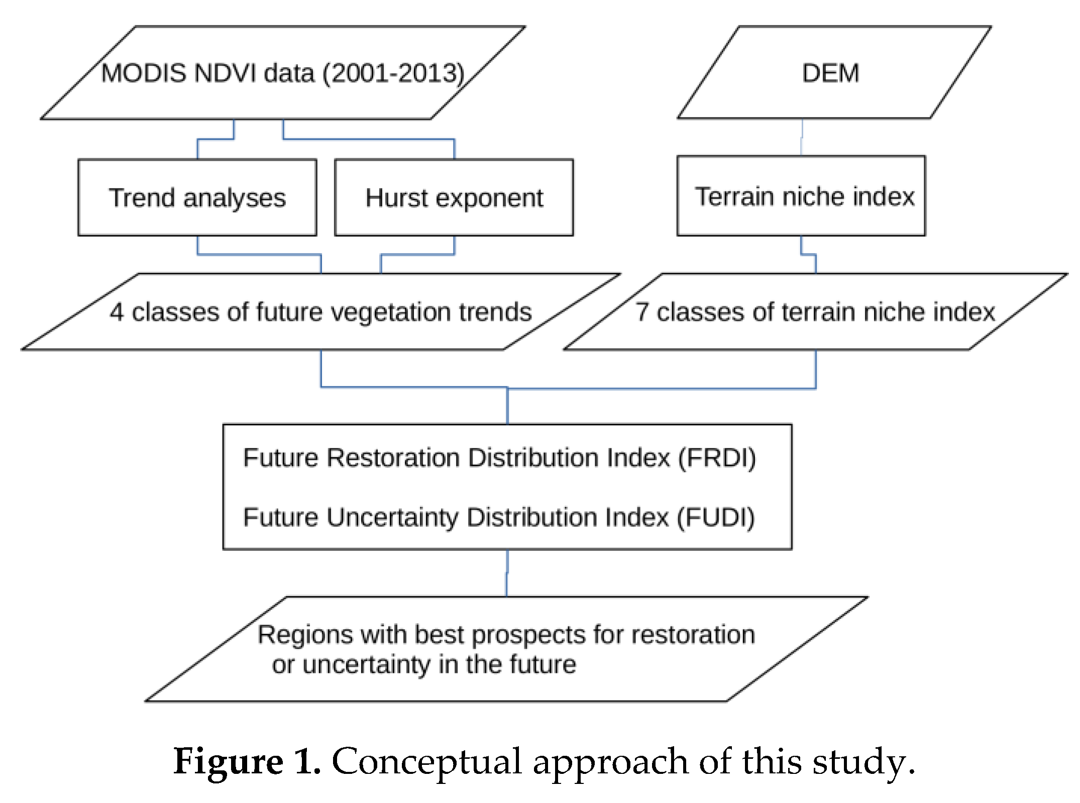
MODIS NDVI data are utilized to generate growing season NDVI (GSN) for each year from 2001 to 2013 to identify regions with the best prospects/high uncertainty for future vegetation restoration in Southwest China (Figure 1). Linear trend analysis and Hurst exponent are used to produce maps of vegetation trends and their persistence. Based on this, a future vegetation trend is generated. Elevation and slope are extracted from a digital elevation model (DEM) and a terrain niche index (TNI) map is calculated, which is classified into 7 separate classes. Two distribution indexes, namely Future Recovery Distribution Index (FRDI) and Future Uncertainty Distribution Index (FUDI), are proposed to explore the distribution of future vegetation dynamics and to identify areas where vegetation has the best prospects for restoration or where future trends are uncertain.
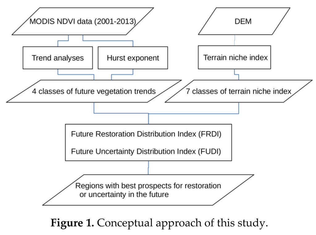
Figure 1.
Conceptual approach of this study.
2.1. Study Area
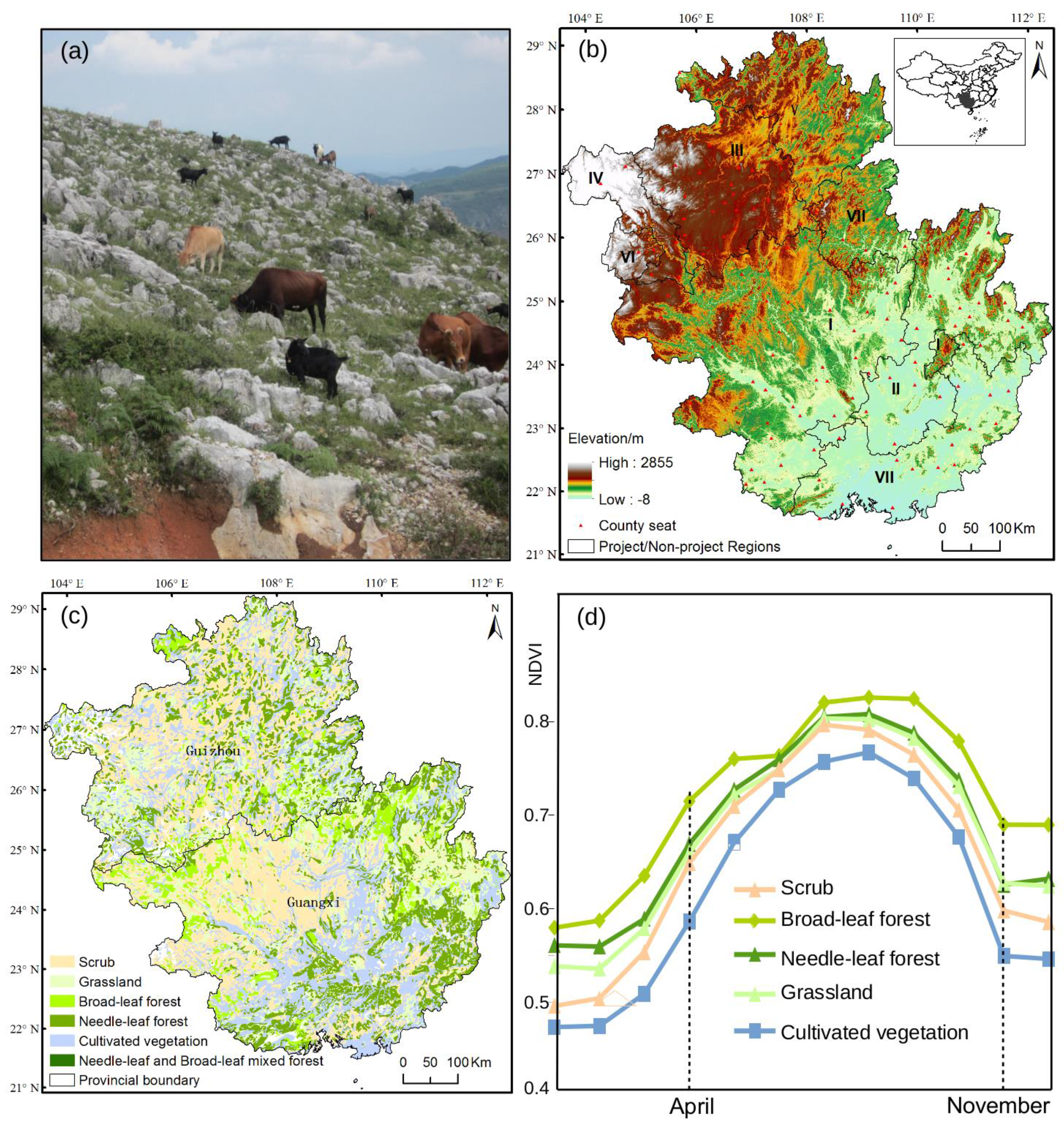
The study area is the Guizhou and Guangxi provinces in Southwest China (20°54′–29°13′N and 103°36′–112°04′E). The area has a total coverage of 4.13 × 10⁵ km2 and a population of 87.84 million people. The elevation ranges from −8 to 2855 m.a.s.l., with maximum heights in the northwest and the minimum in the southeast (Figure 2b). The climate is a subtropical and tropical monsoon climate, with 1465 mm falling during the growing season from April to November. The precipitation from April to September accounts for 70%–85% of the annual total precipitation [45] and the mean growing season temperature is 25 °C. A Total of 45% and 15% of the bedrocks are pure carbonate and impure carbonate (karst region), respectively. The fragile soils of the karst areas are prone to rocky degradation if over-utilized (e.g., by livestock farming, Figure 2a). The bedrock for the rest of the region consists of clastic rocks (non-karst region) [46]. Governmental rocky desertification control projects implemented in karst regions can be divided into six main project regions [47] shown in Figure 2b. The main vegetation cover types are cultivated vegetation (29%), scrub (28%), grassland (17%), needle-leaf forest (16%), and broad-leaf forest (5%) (Figure 2c). Although the seasonal cycle of the main vegetation types differs, the general pattern is uniform, reflecting a growing season from April to November (Figure 2d).

Figure 2.
Rocky karst landscape in Southwest China used for livestock grazing (photo taken in August 2014, Tong). (a) Location of the study area and the distribution of project regions and county seats overlaying a digital elevation model (DEM); (I) peak cluster depression; (II) peak forest plain; (III) karst plateau; (IV) karst gorge; (V) karst trough valley; (VI) karst basin and (VII) non-project regions respectively (b); The spatial distribution of vegetation cover types is shown in (c); The seasonal variations of the main vegetation types based on the mean monthly NDVI from 2001 to 2013 (d).
2.2. Data and Processing
NDVI data used in this study are MODIS (MOD13Q1) from 2001 to 2013 with a temporal resolution of 16 days. The images have a spatial resolution of 250 m and are retrieved from daily, atmospherically corrected surface reflectance. They have been composited using methods based on product quality assurance metrics to remove low quality pixels and the highest quality pixels were chosen for each 16 day composite [48]. For this study, we used the maximum value composite (MVC) method to select the higher value of two 16-day composite images and obtain the monthly NDVI. This further minimizes atmospheric and scan/angle effects, cloud contamination and high solar zenith angle effects [49]. Then the NDVI values from April to November were averaged to obtain the GSN for each year from 2001 to 2013 (see Figure 2d).
A SRTM DEM with 90 m resolution was downloaded from the International Scientific Data Service Platform [50] and used as the source for elevation and slope. The DEM was resampled to 250 m spatial resolution using a nearest neighbor resampling algorithm to match the MODIS NDVI data.
Monthly temperature and rainfall data for 53 weather stations from 2001 to 2013 were obtained from the China Meteorological Data Sharing Service System [51]. The human population data in 2005 and 2010 were provided by the Data Center for Resources and Environmental Sciences, Chinese Academy of Sciences (RESDC) [52].
2.3. Methods
A linear regression between annual GSN and time was applied to derive the slope as an indication of the direction and magnitude of linear trends in the time series. Whereas a positive slope value indicates a positive trend in vegetation (e.g., successful conservation projects), a negative slope value refers to negative vegetation trends which can be an indicator of degradation (e.g., erosion due to anthropogenic overuse). The trends are considered statistically significant if the p value of the regression is smaller than 0.05. If the p value is larger 0.05, no significant change is detected and the pixel is considered to be stable. We thus categorize GSN trends as three types: increasing (slope > 0 and p < 0.05), decreasing (slope < 0 and p < 0.05) and stable (p ≥ 0.05).
The rescaled range (R/S) analysis developed by Hurst is a method used to estimate auto-correlation properties of time series [53]. We apply the Hurst exponent (H), estimated by the R/S analysis, as a measure of the long-term memory in our GSN time series (annual data). The main calculation steps are [54]:
- To divide the time series (τ = 1, 2…, n) into τ sub series , and for each sub series t = 1,…, τ.
- To define the mean sequence of the time series,
- To calculate the cumulative deviation,
- To create the range sequence,
- To create the standard deviation sequence,
- To rescale the range,
The values of the H range between 0 and 1. A value of 0.5 indicates a true random walk. In a random walk there is no correlation between any element and a future element. An H value between 0.5 and 1 (H, 0.5 < H < 1) indicates “persistent behavior” (i.e., a positive autocorrelation). The closer the H values are to 1, the more persistent is the time series. An H value below 0.5 (H, 0 < H < 0.5) means a time series with “anti-persistent behavior” (or negative autocorrelation). The closer the H values are to 0, the more anti-persistent is the time series [55]. The H value was calculated for each pixel to test the persistence of the GSN time series.
Based on the GSN trends and the H value, we categorized the supposed future vegetation trends into six types (Table 1). When a pixel showed a positive trend and its H value was higher than 0.5 (i.e., the positive trend is likely to continue), the vegetation in this pixel is supposed to have an overall positive development (PD) after the time series ends in 2013. If the trend is positive but its H value was less than 0.5 (the positive trend is not likely to continue), the vegetation in this pixel has an anti-persistent positive development (APD) after 2013. When a pixel showed a negative trend and its H value was higher than 0.5 (the negative trend is likely to continue), the vegetation in this pixel is supposed to experience a negative development (ND) after 2013. If the trend is negative and its H value was less than 0.5, (i.e., the negative trend is not likely to continue), the vegetation in this pixel is characterized by an anti-persistent negative development (AND) after 2013. When a pixel was detected to have no significant trend and its H value was higher than 0.5, the vegetation in this pixel is supposed to have a stable and steady development (SSD) after 2013. If its H value was less than 0.5, the future vegetation trend in this pixel is uncertain, which means the trend after 2013 is an undetermined development (UD).

Table 1.
Future vegetation trends based on vegetation dynamics (2001–2013) and the H value.
The terrain niche index (TNI) was utilized to characterize the topographic variation in Southwest China [56]. It was calculated as:
where and are the elevation of the pixel and the average elevation of the study area respectively, whereas and signify the slope of the pixel and the average slope of the study area. Large TNI values correspond to higher elevation and larger slope angles, being typical for karst plateaus and gorges. In contrast, smaller TNI values indicate lower elevation and smaller slope angles. Medium TNI values are found in areas of a higher elevation but small slope angle, or low elevation but with larger slope angles, or moderate elevation and slope angle. In this study the TNI values were categorized into 7 classes with an interval of 0.2.
To characterize the status of the vegetation for each terrain interval beyond 2013, the future vegetation trend classes shown in Table 1 were used as reference. All pixels within each of the 7 terrain intervals were classified according to one of the future trend classes and the overall sum of the classes was calculated (where ND has −1, others have the value 1) for each terrain interval. To account for different area sizes of the terrain intervals and capture supposed future change for each specific interval, we propose two distribution indexes, FRDI (identifying areas where vegetation has the best prospects for restoration) and FUDI (showing the distribution of the uncertainty). These two comprehensive indexes are calculated as follows:
where refers to the 7 terrain intervals; and ( = 1 (PD), 2 (SSD), 3 (ND), 4 (UT), 5 (APD) and 6 (AND)) are the area of the six future vegetation trends (Table 1) in each terrain interval and the study area; and and A refer to the area of the terrain interval and the study area, respectively. and are standardized and dimensionless indexes. If > 1, the corresponding terrain interval is supposed to be more favorable for vegetation restoration in the future than other terrain intervals. The larger the is, the better the future prospect changes. If the is lower than 1, the terrain interval is supposed to have less favorable prospects. If > 1, trend predictions in the terrain interval have a higher uncertainty than other terrain intervals. A lower reduces prediction uncertainty and a below 1 implies more certain prospects.
3. Results
3.1. Vegetation Patterns and Dynamics during 2001–2013
The growing season vegetation in the study area has an average GSN of 0.72 for the period 2001–2013 with a high spatial heterogeneity between the land-cover classes (Figure 3a). For the Guangxi Province, the average GSN is 0.74, which is slightly higher than in the Guizhou Province (0.69). The vegetation type of the needle-leaf and broad-leaf mixed forest class has the highest mean GSN (0.78), followed by broad-leaf forest (0.77), needle-leaf forest (0.74), grassland (0.73), scrub (0.72), and cultivated vegetation (0.68). The average GSN in the non-project region (0.74) is slightly higher than in the project regions (0.71). The regions with a GSN higher than 0.8 are mainly located in Guangxi Province, such as Ninming, Baise, Tianlin, Zhaoping, Cangwu, Tiane, Yongfu County, dominated by broad-leaf forest and needle-leaf forest. The areas with a GSN less than 0.5 are associated with scrubs, cultivated vegetation and built-up areas. These regions are close to roads and railways and correspond to county seats, especially in large cities, such as Nanning, Liuzhou and Guiyang. At the county scale, we found the average GSN of the past 13 years had a significant positive relationship with the distance to roads (p < 0.01) and a significant negative relationship with the population density change from 2005 to 2010 (p = 0.016). Moreover, areas of low GSN are found in mountainous regions dominated by ethnic minorities, such as Weining County populated by the Yi nationality and the Fuchuan County inhabited by the Yao nationality. At the county scale, we found significant positive correlations (p < 0.01) between GSN and growing season climatic factors (temperature and precipitation). GSN was more strongly and positively correlated with temperature (R2 = 0.25) than with precipitation (R2 = 0.11) during 2001–2013.

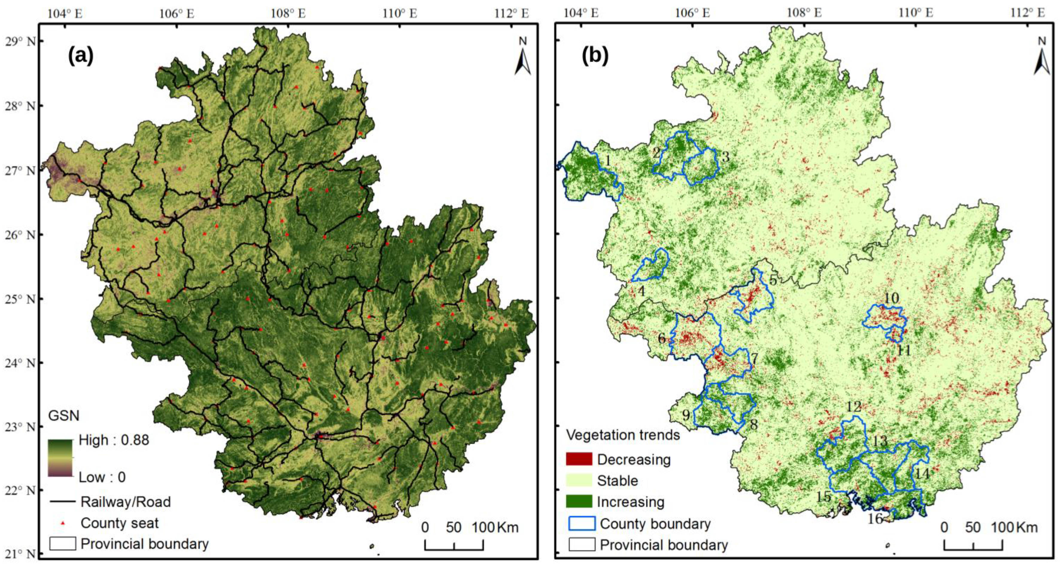
Figure 3.
The vegetation patterns (a) and dynamics (b) in Southwest China based on MODIS NDVI from 2001 to 2013. The numbers in (b) represent counties: (1) Weining; (2) Dafang; (3) Qianxi; (4) Xingren; (5) Tiane; (6) Tianlin; (7) Baise; (8) Debao; (9) Jingxi; (10) Liucheng; (11) Liuzhou; (12) Yongning; (13) Lingshan; (14) Pubei; (15) Qinzhou; (16) Hepu.
Figure 3b shows the trends in annual GSN with distinct spatial differences. An uptrend (slope > 0) is found in 67% of the study area, with 23% of these trends being significant (p < 0.05). These pixels are mainly in Qinzhou and Beihai of Guangxi and Bijie of Guizhou, where the dominant vegetation types are scrubs and cultivated vegetation (i.e., agro-forestry, such as eucalyptus plantation and oil-tea camellia plantation). Furthermore, 33% of the pixels are detected to have a downtrend (slope < 0), with 10% being significant. These pixels are mainly located in Baise and Liuzhou, Guangxi. In addition, the dominating vegetation types of these areas are cultivated vegetation, scrubs and grasslands. Consequently, three vegetation trend types, increasing, decreasing and stable (not significant; p ≥ 0.05) accounted for 15%, 3% and 82%, respectively.
3.2. Future Vegetation Trends after 2013
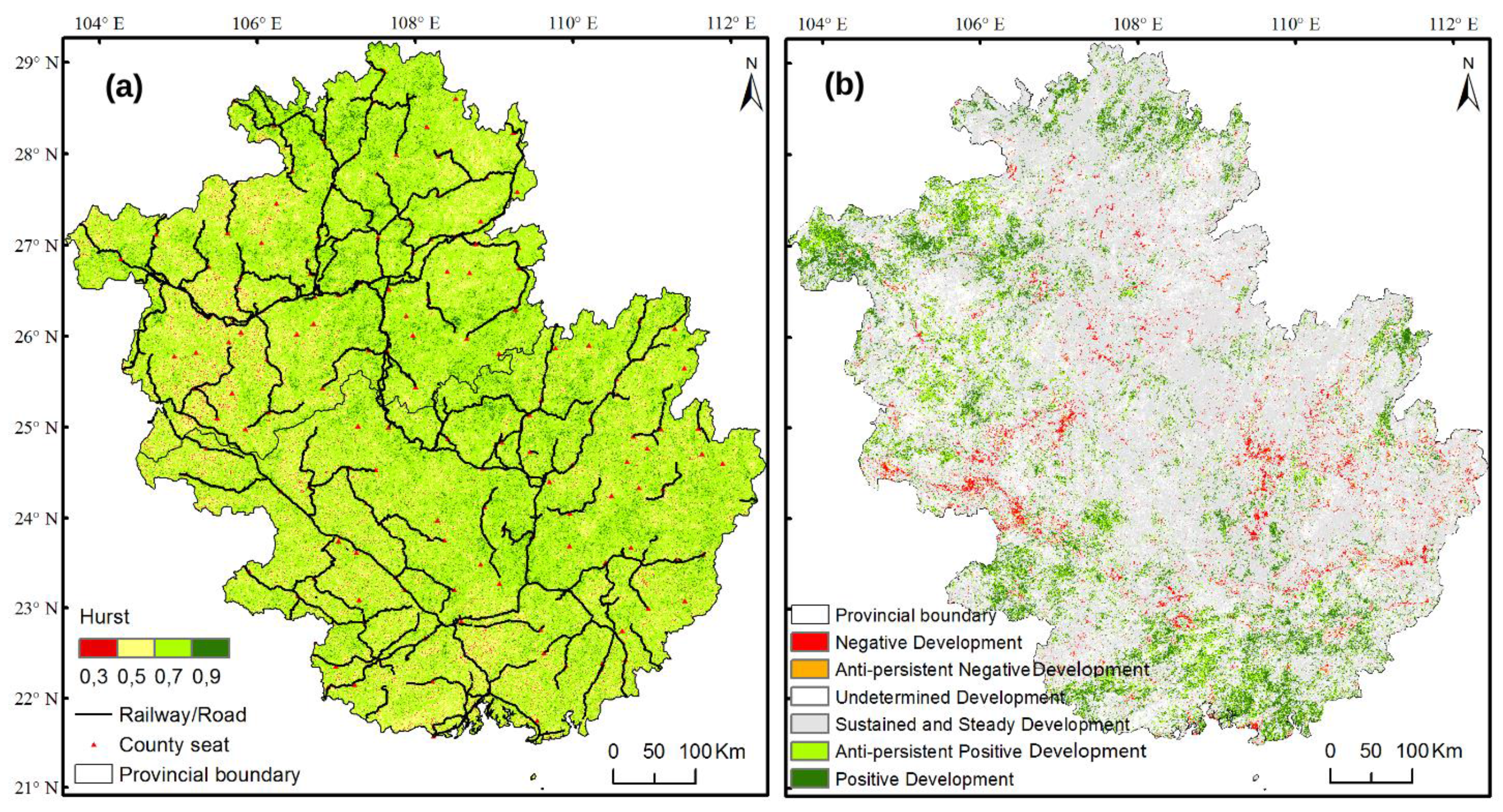
Values of the H range from 0.02 to 0.86 (Figure 4a). The mean H value of the whole study area is 0.55, indicating an overall moderately persistent vegetation trend in the two provinces in Southwest China, suggesting that future vegetation trends are likely to be similar to those of the past 13 years. In particular, the H values between most of the vegetation cover types are relatively similar: broad-leaf forest has a mean H value (0.552), followed by needle-leaf forest (0.551), grassland (0.548), scrub (0.547), and cultivated vegetation (0.546). Only the class needle-leaf and broad-leaf mixed forest is below 0.5 (0.473). In 69% of the study area the H value is above 0.5. Areas with a low persistence were located in the west and the south of the study area. In the west, the regions with low H values were mostly corresponding to the road network, while in the south, the regions with low persistence are close to county seats (Figure 4a).
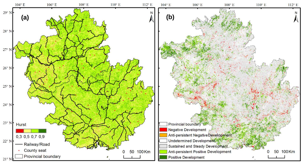
Figure 4.
Maps showing the Hurst exponent (a); and the distribution of future vegetation trends (b) based on observed vegetation trends (2001–2013) in Southwest China.
The vegetation dynamics and the H values were combined into different classes (Table 1) to indicate future vegetation trends (Figure 4b). The future vegetation trends in most parts of the study area (57%) are stable and steady, and particularly vegetation belonging to scrub and cultivated vegetation (Figure 1c) is detected to have no significant trend in the past 13 years and this state will be persistent (H > 0.5). However, 10% of the study area is expected to have a positive development in the future (vegetation had a persistent positive trend). These areas consist primarily of scrubs and are mainly distributed in the north and northwest Guizhou and in southern Guangxi. Areas with a negative development (where vegetation was detected to have a persistent decreasing trend), cover 3% of the study area and the main land cover of these areas is cultivated vegetation. Vegetation showing no trend and no persistence occupy 24% of the study area, where the main land cover types are scrubs and cultivated vegetation. Regions with an anti-persistent negative development cover 1% of the study area. The main land cover of these regions is cultivated vegetation. Areas with an anti-persistent positive development cover 5% of the study area, with scrub being the main land cover class.
3.3. Vegetation Trends and Future Vegetation Trends in Different Project Regions
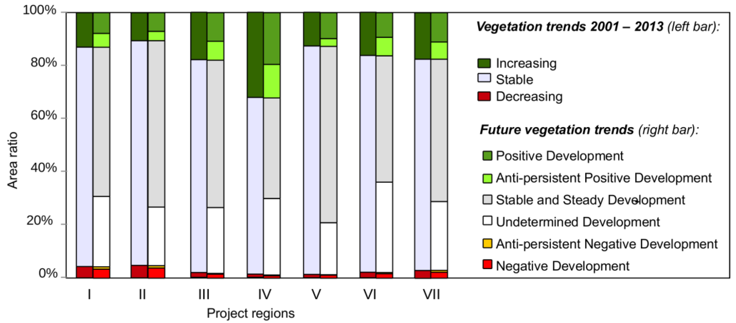
Some differences in vegetation trends and future vegetation trends can be observed (Figure 5) in different regions (Figure 2b). Apart from the karst gorge region (IV) and non-project region (VII), vegetation in 80% of other project regions is rather stable. Vegetation in 32% of the karst gorge region (IV) (having the lowest average GSN with 0.62) shows a significant increasing trend, indicating an improvement of the vegetation in this region. Overall, only a small percentage of the pixels in the project regions have a decreasing trend. With 5% in the peak forest plain region (II), 4% in the peak cluster depression region (I) and 3% in the non-project region (VII), these regions are the only ones with a noticeable share of pixels characterized by significant decreasing trends.

Figure 5.
The area ratio (percentage cover) of different vegetation trends (2001 to 2013) (left bar) and future vegetation trends (right bar) in different project regions (see Figure 2b).
The future vegetation trends with a stable and steady development after 2013 cover 58% and 54% of all project region and non-project region pixels, respectively. In particular, the karst trough valley region (V) and the peak forest plain region (II) account for 66% and 63% respectively, having the highest share of steady trends among the project regions. Overall, 19% of the karst gorge region (IV) and 11% of the karst plateau region (III) are predicted to have a positive development after 2013. However, 37% of the overall positive trends are anti-persistent. In particular, the karst gorge region (IV) needs attention, with 13% of the vegetation showing a positive but anti-persistent development. A total of 25% of the pixels in the project regions have an undetermined trend. More specifically, in 34% of the karst basin region (VI) and 28% of the karst gorge region (IV), the future vegetation trends cannot be determined. The highest share of negative development was found in the peak forest plain region (II) (4%). In general, the share of anti-persistent negative development is small for all project regions (0.5%), indicating some efforts in preventing degradation.
3.4. Distribution of Future Vegetation Trends for Different Terrain Conditions
The TNI values in the study area (ranging from −0.0006 to 1.4) show a pattern of decrease from the northwest to the southeast (Figure 6a), which in general is consistent with the distribution of elevation and slope. The karst gorge region (IV) has the highest TNI (0.85), followed by the karst basin region (VI) (0.84), the karst plateau region (III) (0.70), the karst trough valley region (V) (0.67), the peak cluster depression region (I) (0.54), and the peak forest plain region (II) (0.40). The distribution of future vegetation trends varies between TNI groups (i.e., with the terrain) (Figure 6b). The largest shares of negative and positive development are found in regions with low elevation and slope, which are also the areas characterized by the highest anthropogenic influence. The negative development decreases and the undetermined development increases as the TNI increases. This indicates a decline of anthropogenic impact in rough terrain and a more difficult prediction of future trends.
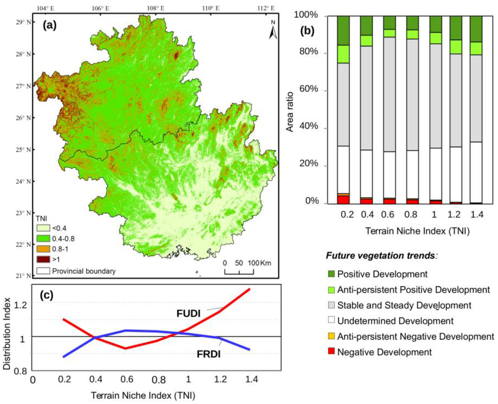
Figure 6.
The terrain niche index (TNI) in Southwest China based on DEM data (a); the area ratio of future vegetation trends for different TNI intervals (b); and the distribution of FRDI and FUDI in different terrain niche indexes (TNI’s) (c).
The distribution of the FRDI and FUDI along the seven terrain intervals (Figure 6c) shows that FRDI (representing the areas with best future prospects) is low in areas with a low TNI but is larger than 1 when the TNI is in the range between 0.4 and 1 (areas with a moderate slope and elevation). The uncertainty for future predictions (FUDI) is high in areas of low TNI, but low in areas with a TNI between 0.4 and 1, being in line with the FRDI. Thus, these terrain niche intervals are identified as regions with the best prospects for vegetation restoration in the future. The FUDI increases again with higher TNI, indicating that regions with a small slope and low elevation or a large slope and high elevation contain the highest uncertainty in future prospects.
Most pixels with TNI between 0.4 and 1 are found in the peak cluster depression region (I) (36%), the karst plateau region (III) (19%) and the karst trough valley region (V) (16%) (Figure 7a). Therefore, the future vegetation restoration has the best prospects in these project regions. The areas with a TNI greater than 0.8 are mainly distributed in the peak cluster depression region (I) (25%), the karst plateau region (III) (19%) and the karst gorge region (IV) (17%). The future vegetation trends in these project regions have a high uncertainty. However, based on the ratio of each terrain interval in every project region (Figure 7b), we found the largest share of TNI between 0.4 and 1 in the karst plateau region (III) (95%) and the karst trough valley region (V) (89%). Thus, the share of pixels prospecting from future vegetation restoration in the karst plateau region (III) and the karst trough valley region (V) will be greater than in other regions. The largest shares of TNI greater than 0.8 are found in the karst gorge region (IV) (62%) and the karst basin region (VI) (61%), while the largest shares of TNI smaller than 0.2 are found in the non-project region (VII) (35%) and the peak forest plain region (II) (33%). Both high and low TNI values indicate a high future vegetation uncertainty in these regions.
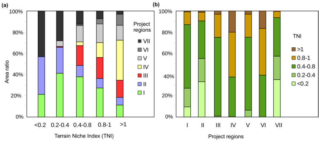
Figure 7.
The ratio of pixels per TNI interval for the different project/non-project regions (a) and the ratio of pixels per region for the different TNI intervals (b).
3.5. Validation of the Method
The time series was split into two parts (2001–2007 and 2008–2013) and pixels with a significant (p < 0.05) trend for both periods were chosen for validating the future trend prediction methodology (Table 2). In spite of the short time periods, the prediction performs well for most classes—only the prediction for negative persistent trends does not apply.
Table 2.
For validation, the time series was split into two periods and pixels with significant (p < 0.05) trends in both periods were analyzed. Due to the short periods, the numbers of pixels meeting these assumptions are limited (shown in brackets in the first column). The mean slopes (GSN year−1) for these pixels (both periods) are shown. The predictions are based on the first period (2001 to 2007).
4. Discussion
4.1. Drivers of Vegetation Conditions and Dynamics
Many studies have suggested that climate change is one of the main drivers of trends in vegetation productivity in China [57,58]. However, in our study the role of average growing season temperature and precipitation is limited since the coefficients of determination of both relationships are rather low (yet statistically significant), confirming the results of Hou et al. [59]. Furthermore, the relationship between GSN and precipitation is weaker than for temperature, which is consistent with the study by Wang et al. [60]. This might be due to Southwest China being located in the subtropical monsoon climate zone, with rich precipitation and moderate temperature, and thereby slight changes in precipitation will not heavily affect vegetation growth. On the other hand, the above and below-ground hydrological structures of the karst region leads to a significant drain and runoff [61], which suggests that precipitation cannot be effectively utilized for vegetation growth.
Anthropogenic influences, such as ecological projects, population growth, and urbanization, were found to be more important factors that affect vegetation change [62,63,64,65]. A few previous studies highlighted the positive impacts of ecological restoration projects on vegetation dynamics [66,67,68,69]. The accumulative afforested area by aerial seeding and forest plantation in Southwest China had increased quickly from 65,744 ha in 2000 to 1,709,366 ha in 2011. Furthermore, the overall deteriorated trends of rocky desertification had been transformed from net increase to net decrease since 2011 in karst regions, Southwest China [70]. With the implementation of the Karst Rocky Desertification Comprehensive Control and Restoration Project, the soil fertility and surface vegetation cover rate in karst regions have been improved [71,72,73]. Partly due to the ecological projects in the past 15 years, most vegetation communities in the present study area have achieved a stable growing stage with a relatively high GSN and show thus no significant trend (Figure 3b). However, some regions with a significant decrease in vegetation have been detected. These areas are usually around county seats or in proximity to roads, identifying rapid urbanization and road construction to lead to the degradation of vegetation. Generally, the average cover and successional rate of vegetation are lower in karst regions as compared to non-karst regions [74]. In our study, the average GSN in project regions (karst region) is still lower than in non-project region (non-karst region). However, the annual increase of GSN from 2001 to 2013 in project regions (0.0024 GSN year−1) is higher than in non-project region (0.0023 GSN year−1), indicating that vegetation cover grows more quickly under the implementation of ERPs.
4.2. Influence of Terrain Conditions on Vegetation Distribution
A framework for governmental decision makers is proposed to highlight regions that need more attention when implementing ecological projects. The FRDI and FUDI indexes, based on the future vegetation trends and the TNI, were utilized to detect specific areas where vegetation had the best prospects to be restored or the highest uncertainty in the future. The results showed that regions with a TNI between 0.4 and 1 were the most advantageous intervals for vegetation restoration in the future. In the past 13 years, the average growing season temperature and precipitation dropped as the TNI increased. In regions with TNI less than 0.4, the average growing season temperature and precipitation are 28 °C and 1721 mm respectively, whereas in regions with TNI between 0.4 and 1, averages are 25 °C and 1355 mm, and in regions with TNI greater than 1, 20 °C and 1218 mm. In the region studied, areas with a low TNI (less than 0.4) have the best combined conditions of air temperature and water favoring vegetation growth. In addition, the Returning Farmland to Forest Program has been implemented in regions with slope greater than 25°, which supports vegetation restoration. Therefore, vegetation in these regions is likely to have reached a stable condition, and the room for further improvement is less than in other regions. The conditions of air temperature and water in regions with a TNI between 0.4 and 1 are less ideal compared to areas with a lower TNI but better than for areas with a higher TNI. Therefore, vegetation in these regions has a higher chance of improvement under the implementation of projects than in regions with a higher TNI. According to the distribution of FUDI in areas with different TNIs, vegetation development in regions with a high TNI (greater than 0.8) has a higher uncertainty. These regions with high elevation and large slope angles can induce soil erosion under heavy rainfall. Besides, vegetation in these areas suffers more easily under droughts since the steep terrain condition is not suitable for water conservation [75]. Thus, vegetation in these regions is likely to be more strongly influenced by climatic conditions than other regions and fluctuate along with climate variations. Areas with TNI smaller 0.2 are found in the non-project region (VII) and the peak forest plain region (II). These areas are well suited for vegetation growth and are characterized by high anthropogenic influence. The anthropogenic disturbances lead to a generally uncertain (reflected in a high FUDI) and negative vegetation development.
4.3. Limitations and Future Research Directions
For validation, the time series was divided into two periods. Results showed that the prediction performs well for most classes except the prediction for negative persistent trends. This could be interpreted as an indication of the successful implementation of anthropogenic projects preventing further degradation. However, both periods are rather short due to the length of the full time series based on the use of MODIS data (2000–2013). Thus, the validation is based on trends and predictions characterized by high uncertainty and a longer time series is needed for a more robust validation. Moreover, the TNI was utilized to characterize the terrain conditions and the two indexes (FRDI and FUDI) were an effective approach for identifying the most advantageous intervals for vegetation restoration in the future and the corresponding prediction uncertainty. However, we were not able to quantify the specific elevation and slope of these regions. Thus, more work is needed to analyze the relationship between the vegetation variations and topographical conditions and to explore the exact ranges of elevation and slope suited for specific purposes. The variations of the vegetation trends were affected by climate and human activities, especially national/local policies. We explored the driving forces associated with vegetation variations but did not statistically distinguish the effects caused by climate and human activities on vegetation dynamics, which facilitates a quantification of the efficiency of human-induced effort on vegetation restoration.
5. Summary and Conclusions
- (1)
- Overall, Southwest China was shown to be characterized by good vegetation condition during 2001 and 2013 without signs of widespread vegetation degradation. The average temperature and precipitation of a growing season were shown to have limited impact on vegetation change. Road construction and increasing urbanization have led to vegetation with lower growing season Normalized Difference Vegetation Index, such as scrubs and cultivated vegetation.
- (2)
- Most of the vegetation shows no significant trend in the past 13 years. The percentage of pixels with an increasing trend is greater than that of decreasing trends. The karst gorge region has the largest share of increasing trends amongst the 6 project regions. The peak forest plain region and the peak cluster depression region are found to have a noticeable share of pixel showing a significant decreasing trend.
- (3)
- The vegetation trends in Southwest China are rather persistent. For the whole study area, the future vegetation with a stable and steady development is dominant, especially in the karst trough valley and the peak forest plain. The percentage of vegetation with positive development is greater than that of negative development. The karst gorge has the highest share of pixels showing positive development and anti-persistent development. The karst peak forest plain region has the highest share of pixels with negative development. The karst basin has the highest share of pixels characterized by an undetermined trend.
- (4)
- Most negative future development is found in areas of high anthropogenic influence, as compared to areas of rough terrain.
- (5)
- The regions with terrain niche index (TNI) between 0.4 and 1 have the best prospects for vegetation restoration in the future (especially in the karst plateau region and the karst trough valley region). Moreover, regions with TNI greater than 1 show the highest uncertainty for future prospects (especially in the karst gorge region and the karst basin region). It is here suggested that governmental restoration projects should duly pay attention to these regions to prevent vegetation degradation.
- (6)
- We have shown that the framework of the present analysis works well for assessing restoration prospects in the study area. Due to its generic design, the method used is expected to be applicable for studies located in other areas of complex landscapes in the world, exploring future vegetation trends.
Acknowledgments
This work was supported by the National Natural Science Foundation of China (Grant No. 41471445, 41371418), Science and Technology Service Network Initiative (No. KFJ-EW-STS-092), Chinese Academy of Sciences “Light of West China” Program, and European Union’s Horizon 2020 research and innovation programme under the Marie Sklodowska-Curie (Grant No. 656564). The authors wish to thank MODIS NDVI Group for producing and sharing the NDVI dataset. NASA and NIMA are thanked for sharing DEM data. The team behind the weather data is thanked for sharing the climatic data. The authors want to thank Yanfang Xu for helping with data processing, and Chunhua Zhang and Mingyang Zhang for their helpful comments on the manuscript. We also thank the journal editor and the anonymous reviewers for their useful comments and great efforts on this paper.
Author Contributions
All authors contributed significantly to this manuscript. To be specific, Kelin Wang and Yuemin Yue designed this study. Xiaowei Tong and Chujie Liao were responsible for the data processing and analysis. Xiaowei Tong wrote the draft with support of Martin Brandt and Rasmus Fensholt.
Conflicts of Interest
The authors declare no conflict of interest.
References
- Arora, V. Modeling vegetation as a dynamic component in soil-vegetation-atmosphere transfer schemes and hydrological models. Rev. Geophys. 2002, 40. [Google Scholar] [CrossRef]
- Douville, H.; Planton, S.; Royer, J.-F.; Stephenson, D.B.; Tyteca, S.; Kergoat, L.; Lafont, S.; Betts, R.A. Importance of vegetation feedbacks in doubled-CO2 climate experiments. J. Geophys. Res. Atmos. 2000, 105, 14841–14861. [Google Scholar] [CrossRef]
- Eugster, W.; Rouse, W.R.; Pielke, S.R.A.; Mcfadden, J.P.; Baldocchi, D.D.; Kittel, T.G.F.; Chapin, F.S.; Liston, G.E.; Vidale, P.L.; Vaganov, E.; et al. Land-atmosphere energy exchange in Arctic tundra and boreal forest: Available data and feedbacks to climate. Glob. Chang. Biol. 2000, 6, 84–115. [Google Scholar] [CrossRef]
- Suzuki, R.; Masuda, K.; Dye, D.G. Interannual covariability between actual evapotranspiration and PAL and GIMMS NDVIs of northern Asia. Remote Sens. Environ. 2007, 106, 387–398. [Google Scholar] [CrossRef]
- Kelly, M.; Tuxen, K.A.; Stralberg, D. Mapping changes to vegetation pattern in a restoring wetland: Finding pattern metrics that are consistent across spatial scale and time. Ecol. Indic. 2011, 11, 263–273. [Google Scholar] [CrossRef]
- Jiang, Z.C.; Lian, Y.Q.; Qin, X.Q. Rocky desertification in Southwest China: Impacts, causes, and restoration. Earth Sci. Rev. 2014, 132, 1–12. [Google Scholar] [CrossRef]
- Daoxian, Y. Rock Desertification in the Subtropical Karst of South China; Gerbüder Borntraeger: Stuttgart, Germany, 1997. [Google Scholar]
- Chinese Academy of Sciences. Several suggestions for the comprehensive taming to karst mountain areas in Southwest China. Bull. Chin. Acad. Sci. 2003, 3, 169. [Google Scholar]
- Yue, Y.M.; Zhang, B.; Wang, K.L.; Liu, B.; Li, R.; Jiao, Q.J.; Yang, Q.Q.; Zhang, M.Y. Spectral indices for estimating ecological indicators of karst rocky desertification. Int. J. Remote Sens. 2010, 31, 2115–2122. [Google Scholar] [CrossRef]
- Huang, Q.H.; Cai, Y.L. Spatial pattern of karst rock desertification in the middle of Guizhou Province, Southwestern China. Environ. Geol. 2006, 52, 1325–1330. [Google Scholar] [CrossRef]
- Pettorelli, N.; Vik, J.O.; Mysterud, A.; Gaillard, J.-M.; Tucker, C.J.; Stenseth, N.C. Using the satellite-derived NDVI to assess ecological responses to environmental change. Trends Ecol. Evol. 2005, 20, 503–510. [Google Scholar] [CrossRef] [PubMed]
- Tucker, C.J.; Vanpraet, C.L.; Sharman, M.J.; Van Ittersum, G. Satellite remote sensing of total herbaceous biomass production in the Senegalese Sahel: 1980–1984. Remote Sens. Environ. 1985, 17, 233–249. [Google Scholar] [CrossRef]
- Badeck, F.W.; Bondeau, A.; Böttcher, K.; Doktor, D.; Lucht, W.; Schaber, J.; Sitch, S. Responses of spring phenology to climate change. New Phytol. 2004, 162, 295–309. [Google Scholar] [CrossRef]
- Levin, N.; Shmida, A.; Levanoni, O.; Tamari, H.; Kark, S. Predicting mountain plant richness and rarity from space using satellite-derived vegetation indices. Divers. Distrib. 2007, 13, 692–703. [Google Scholar] [CrossRef]
- Ma, W.; Fang, J.; Yang, Y.; Mohammat, A. Biomass carbon stocks and their changes in northern China’s grasslands during 1982–2006. Sci. China Life Sci. 2010, 53, 841–850. [Google Scholar] [CrossRef] [PubMed]
- Myneni, R.B.; Keeling, C.D.; Tucker, C.J.; Asrar, G.; Nemani, R.R. Increased plant growth in the northern high latitudes from 1981 to 1991. Nature 1997, 386, 698–702. [Google Scholar] [CrossRef]
- Tucker, C.J.; Slayback, D.A.; Pinzon, J.E.; Los, S.O.; Myneni, R.B.; Taylor, M.G. Higher northern latitude normalized difference vegetation index and growing season trends from 1982 to 1999. Int. J. Biometeorol. 2001, 45, 184–190. [Google Scholar] [CrossRef] [PubMed]
- Nemani, R.R.; Keeling, C.D.; Hashimoto, H.; Jolly, W.M.; Piper, S.C.; Tucker, C.J.; Myneni, R.B.; Running, S.W. Climate-driven increases in global terrestrial net primary production from 1982 to 1999. Science 2003, 300, 1560–1563. [Google Scholar] [CrossRef] [PubMed]
- Cleland, E.E.; Chuine, I.; Menzel, A.; Mooney, H.A.; Schwartz, M.D. Shifting plant phenology in response to global change. Trends Ecol. Evol. 2007, 22, 357–365. [Google Scholar] [CrossRef] [PubMed]
- Fensholt, R.; Proud, S.R. Evaluation of Earth Observation based global long term vegetation trends—Comparing GIMMS and MODIS global NDVI time series. Remote Sens. Environ. 2012, 119, 131–147. [Google Scholar] [CrossRef]
- Wu, Z.T.; Wu, J.J.; Liu, J.H.; He, B.; Lei, T.J.; Wang, Q.F. Increasing terrestrial vegetation activity of ecological restoration program in the Beijing–Tianjin sand source region of China. Ecol. Eng. 2013, 52, 37–50. [Google Scholar] [CrossRef]
- Zheng, Y.F.; Liu, H.J.; Wu, R.J.; Wu, Z.P.; Niu, N.Y. Correlation between NDVI and principal climate factors in Guizhou Province. J. Ecol. Rural Environ. 2009, 25, 12–17. (In Chinese) [Google Scholar]
- Zhang, Y.D.; Zhang, X.H.; Liu, S.R. Correlation analysis on normalized difference vegetation index (NDVI) of different vegetations and climatic factors in Southwest China. Chin. J. Appl. Ecol. 2011, 22, 323–330. (In Chinese) [Google Scholar]
- Li, H.; Cai, Y.L.; Chen, R.S.; Chen, Q.; Yan, X. Effect assessment of the project of grain for green in the karst region in Southwestern China: A case study of Bijie Prefecture. Acta Ecol. Sin. 2011, 31, 3255–3264. (In Chinese) [Google Scholar]
- Yang, S.F.; An, Y.L. Spatial and temporal variations of vegetation coverage in karst areas under the background of ecological recovery: A case study in the central area of Guizhou Province. Earth Environ. 2014, 42, 404–412. (In Chinese) [Google Scholar] [CrossRef]
- Tong, X.W.; Wang, K.L.; Yue, Y.M.; Liao, C.J.; Xu, Y.F.; Zhu, H.T. Trends in vegetation and their responses to climate and topography in northwest Guangxi. Acta Ecol. Sin. 2014, 34, 1–10. (In Chinese) [Google Scholar]
- Mantegna, R.N.; Stanley, H.E. An Introduction to Econophysics: Correlations and Complexity in Finance; Cambridge University Press: Cambridge, UK, 2000. [Google Scholar]
- Grau-Carles, P. Empirical evidence of long-range correlations in stock returns. Phys. Stat. Mech. Appl. 2000, 287, 396–404. [Google Scholar] [CrossRef]
- Mandelbrot, B.B.; Richard, L.H. The (Mis) Behavior of Markets; Basic Books: New York, NY, USA, 2004. [Google Scholar]
- Rangarajan, G.; Sant, D.A. Fractal dimensional analysis of Indian climatic dynamics. Chaos Solitons Fractals 2004, 19, 285–291. [Google Scholar] [CrossRef]
- Hirabayashi, T.; Ito, K.; Yoshii, T. Multifractal analysis of earthquakes. Pure Appl. Geophys. 1992, 138, 591–610. [Google Scholar] [CrossRef]
- Carbone, A.; Castelli, G.; Stanley, H.E. Time-dependent Hurst exponent in financial time series. Phys. Stat. Mech. Appl. 2004, 344, 267–271. [Google Scholar] [CrossRef]
- Peng, J.; Liu, Z.H.; Liu, Y.H.; Wu, J.S.; Han, Y.N. Trend analysis of vegetation dynamics in Qinghai–Tibet Plateau using Hurst Exponent. Ecol. Indic. 2012, 14, 28–39. [Google Scholar] [CrossRef]
- Li, S.S.; Yan, J.P.; Liu, X.Y.; Wan, J. Response of vegetation restoration to climate change and human activities in Shaanxi-Gansu-Ningxia Region. J. Geogr. Sci. 2013, 23, 98–112. [Google Scholar] [CrossRef]
- Miao, L.J.; Jiang, C.; Xue, B.L.; Liu, Q.; He, B.; Nath, R.; Cui, X. Vegetation dynamics and factor analysis in arid and semi-arid Inner Mongolia. Environ. Earth Sci. 2014, 73, 2343–2352. [Google Scholar] [CrossRef]
- Seddon, A.W.R.; Macias-Fauria, M.; Long, P.R.; Benz, D.; Willis, K.J. Sensitivity of global terrestrial ecosystems to climate variability. Nature 2016, 531, 229–232. [Google Scholar] [CrossRef] [PubMed]
- Bledsoe, B.P.; Shear, T.H. Vegetation along hydrologic and edaphic gradients in a North Carolina coastal plain creek bottom and implications for restoration. Wetlands 2000, 20, 126–147. [Google Scholar] [CrossRef]
- Pabst, H.; Kühnel, A.; Kuzyakov, Y. Effect of land-use and elevation on microbial biomass and water extractable carbon in soils of Mt. Kilimanjaro ecosystems. Appl. Soil Ecol. 2013, 67, 10–19. [Google Scholar] [CrossRef]
- Tsui, C.C.; Tsai, C.C.; Chen, Z.S. Soil organic carbon stocks in relation to elevation gradients in volcanic ash soils of Taiwan. Geoderma 2013, 209–210, 119–127. [Google Scholar] [CrossRef]
- Liu, Q.J.; An, J.; Wang, L.Z.; Wu, Y.Z.; Zhang, H.Y. Influence of ridge height, row grade, and field slope on soil erosion in contour ridging systems under seepage conditions. Soil Tillage Res. 2015, 147, 50–59. [Google Scholar] [CrossRef]
- Moore, I.D.; Gessler, P.E.; Nielsen, G.A.; Peterson, G.A. Soil attribute prediction using terrain analysis. Soil Sci. Soc. Am. J. 1993, 57, 443–452. [Google Scholar] [CrossRef]
- Florinsky, I.V.; Kuryakova, G.A. Influence of topography on some vegetation cover properties. CATENA 1996, 27, 123–141. [Google Scholar] [CrossRef]
- Ohsawa, T.; Saito, Y.; Sawada, H.; Ide, Y. Impact of altitude and topography on the genetic diversity of Quercus serrata populations in the Chichibu Mountains, central Japan. Flora Morphol. Distrib. Funct. Ecol. Plants 2008, 203, 187–196. [Google Scholar] [CrossRef]
- Laamrani, A.; Valeria, O.; Bergeron, Y.; Fenton, N.; Cheng, L.Z.; Anyomi, K. Effects of topography and thickness of organic layer on productivity of black spruce boreal forests of the Canadian Clay Belt region. For. Ecol. Manag. 2014, 330, 144–157. [Google Scholar] [CrossRef]
- Lian, Y.Q.; You, G.J.Y.; Lin, K.R.; Jiang, Z.C.; Zhang, C.; Qin, X.Q. Characteristics of climate change in southwest China karst region and their potential environmental impacts. Environ. Earth Sci. 2014, 74, 937–944. [Google Scholar] [CrossRef]
- Tong, L.Q.; Liu, C.L.; Nie, H.F. Remote Sensing Investigation and Study on the Evolution of China South Karst Rocky Desertification Areas; Science Press: Beijing, China, 2009. [Google Scholar]
- Yuan, D.X. The Research and Countermeasures of Major Environmental Geological Problems in Karst Areas of Southwest China; Science Press: Beijing, China, 2014. [Google Scholar]
- Vermote, E.F.; Saleous, N.Z.; Justice, C.O. Atmospheric correction of MODIS data in the visible to middle infrared: First results. Remote Sens. Environ. 2002, 83, 97–111. [Google Scholar] [CrossRef]
- Holben, B.N. Characteristics of maximum-value composite images from temporal AVHRR data. Int. J. Remote Sens. 1986, 7, 1417–1434. [Google Scholar] [CrossRef]
- International Scientific Data Service Platform. Available online: http://datamirror.csdb.cn/ (accessed on 25 April 2016).
- China Meteorological Data Sharing Service System. Available online: http://cdc.cma.gov.cn (accessed on 25 April 2016).
- Data Center for Resources and Environmental Sciences, Chinese Academy of Sciences (RESDC). Available online: http://www.resdc.cn (accessed on 25 April 2016).
- Hurst, H. Long term storage capacity of reservoirs. Trans. Am. Soc. Civ. Eng. 1951, 6, 770–799. [Google Scholar]
- Sánche Granero, M.A.; Trinidad Segovia, J.E.; García Pérez, J. Some comments on Hurst exponent and the long memory processes on capital markets. Phys. Stat. Mech. Appl. 2008, 387, 5543–5551. [Google Scholar] [CrossRef]
- Mandelbrot, B.B.; Wallis, J.R. Robustness of the rescaled range R/S in the measurement of noncyclic long run statistical dependence. Water Resour. Res. 1969, 5, 967–988. [Google Scholar] [CrossRef]
- Yu, H.; Zeng, H.; Jiang, Z.Y. Study on distribution characteristics of landscape elements along the terrain gradient. Sci. Geogr. Sin. 2001, 21, 64–69. [Google Scholar]
- Zhou, L.; Tucker, C.J.; Kaufmann, R.K.; Slayback, D.; Shabanov, N.V.; Myneni, R.B. Variations in northern vegetation activity inferred from satellite data of vegetation index during 1981 to 1999. J. Geophys. Res. Atmos. 2001, 106, 20069–20083. [Google Scholar] [CrossRef]
- Piao, S.L.; Mohammat, A.; Fang, J.Y.; Cai, Q.; Feng, J.M. NDVI-based increase in growth of temperate grasslands and its responses to climate changes in China. Glob. Environ. Chang. 2006, 16, 340–348. [Google Scholar] [CrossRef]
- Hou, W.J.; Gao, J.B.; Wu, S.H.; Dai, E.F. Interannual variations in growing-season NDVI and its correlation with climate variables in the southwestern karst region of China. Remote Sens. 2015, 7, 11105–11124. [Google Scholar] [CrossRef]
- Wang, J.; Meng, J.J.; Cai, Y.L. Assessing vegetation dynamics impacted by climate change in the southwestern karst region of China with AVHRR NDVI and AVHRR NPP time-series. Environ. Geol. 2007, 54, 1185–1195. [Google Scholar] [CrossRef]
- Du, X.L.; Wang, S.J. Space-time distribution of soil water in a karst area: A case study of the Wangjiazhai catchment, Qinzhen, Guizhou Province. Earth Environ. 2008, 36, 193–201. (In Chinese) [Google Scholar]
- Zhu, H.Y. Underlying motivation for land use change: A case study on the variation of agricultural factor productivity in Xinjiang, China. J. Geogr. Sci. 2013, 23, 1041–1051. [Google Scholar] [CrossRef]
- Liu, J.X.; Li, Z.G.; Zhang, X.P.; Li, R.; Liu, X.C.; Zhang, H.Y. Responses of vegetation cover to the grain for green program and their driving forces in the He-Long region of the middle reaches of the Yellow River. J. Arid Land 2013, 5, 511–520. [Google Scholar] [CrossRef]
- Zhou, S.; Huang, Y.F.; Yu, B.F.; Wang, G.Q. Effects of human activities on the eco-environment in the middle Heihe River Basin based on an extended environmental Kuznets curve model. Ecol. Eng. 2015, 76, 14–26. [Google Scholar] [CrossRef]
- Yu, F.K.; Huang, X.H.; Yuan, H.; Ye, J.X.; Yao, P.; Qi, D.H.; Yang, G.Y.; Ma, J.G.; Shao, H.B.; Xiong, H.Q. Spatial-temporal vegetation succession in Yao’an County, Yunnan Province, Southwest China during 1976–2014: A case survey based on RS technology for mountains eco-engineering. Ecol. Eng. 2014, 73, 9–16. [Google Scholar] [CrossRef]
- Deng, L.; Shangguan, Z.P.; Li, R. Effects of the grain-for-green program on soil erosion in China. Int. J. Sediment Res. 2012, 27, 120–127. [Google Scholar] [CrossRef]
- Sun, Q.Z.; Liu, R.L.; Chen, J.Y.; Zhang, Y.P. Effect of planting grass on soil erodion in karst demonstration areas of rocky desertification integrated rehabilitation in Guizhou province. Soil Water Conserv. 2013, 27, 67–77. (In Chinese) [Google Scholar]
- Xiao, L.; Yang, X.H.; Chen, S.X.; Cai, H.Y. An assessment of erosivity distribution and its influence on the effectiveness of land use conversion for reducing soil erosion in Jiangxi, China. CATENA 2015, 125, 50–60. [Google Scholar] [CrossRef]
- Wang, J.; Wang, K.L.; Zhang, M.Y.; Zhang, C.H. Impacts of climate change and human activities on vegetation cover in hilly southern China. Ecol. Eng. 2015, 81, 451–461. [Google Scholar] [CrossRef]
- The State Forestry Administration of the People’s Republic of China. The Bulletin of Rocky Desertification in China; The State Forestry Administration of the People’s Republic of China: Beijing, China, 2012. (In Chinese)
- Zhang, J. Planning for comprehensive desertification control in karst area of Guangxi Zhuang Autonomous region. Partacult. Sci. 2008, 25, 93–102. (In Chinese) [Google Scholar]
- Yang, Q.Y.; Jiang, Z.C.; Yuan, D.X.; Ma, Z.L.; Xie, Y.Q. Temporal and spatial changes of karst rocky desertification in ecological reconstruction region of Southwest China. Environ. Earth Sci. 2014, 72, 4483–4489. [Google Scholar] [CrossRef]
- Cai, H.Y.; Yang, X.H.; Wang, K.J.; Xiao, L.L. Is forest restoration in the Southwest China karst promoted mainly by climate change or human-induced factors? Remote Sens. 2014, 6, 9895–9910. [Google Scholar] [CrossRef]
- He, Y.B.; Zhang, X.B.; Wang, A.B. Discussion on karst soil erosion mechanism in karst mountain area in southwest China. Ecol. Environ. Sci. 2009, 18, 2393–2398. [Google Scholar]
- Wang, S.Y.; Su, W.C.; Fan, X.R.; Li, C.; Shi, X.T. Influence factors of soil moisture in karst rocky desertification region—A case study of Puding County, Guizhou Province. Res. Soil Water Conserv. 2010, 17, 171–176. [Google Scholar]


© 2016 by the authors; licensee MDPI, Basel, Switzerland. This article is an open access article distributed under the terms and conditions of the Creative Commons Attribution (CC-BY) license (http://creativecommons.org/licenses/by/4.0/).