Article

Optical Models for Remote Sensing of Colored Dissolved Organic Matter Absorption and Salinity in New England, Middle Atlantic and Gulf Coast Estuaries USA

by
Darryl J. Keith
1,*,
Ross S. Lunetta
2 and
Blake A. Schaeffer
2
1
National Health and Environmental Effects Research Laboratory, Office of Research and Development, U.S. Environmental Protection Agency, Atlantic Ecology Division, Narragansett, RI 02882, USA
2
National Exposure Research Laboratory, Office of Research and Development, U.S. Environmental Protection Agency, Environmental Measurements and Methods Division, Research Triangle Park, Durham, NC 27709, USA
*
Author to whom correspondence should be addressed.
Remote Sens. 2016, 8(4), 283; https://doi.org/10.3390/rs8040283
Submission received: 29 December 2015 / Revised: 4 March 2016 / Accepted: 17 March 2016 / Published: 29 March 2016

Abstract

:
Ocean color algorithms have been successfully developed to estimate chlorophyll a and total suspended solids concentrations in coastal and estuarine waters but few have been created to estimate light absorption due to colored dissolved inorganic matter (CDOM) and salinity from the spectral signatures of these waters. In this study, we used remotely sensed reflectances in the red and blue-green portions of the visible spectrum retrieved from Medium Resolution Imaging Spectrometer (MERIS) and the International Space Station (ISS) Hyperspectral Imager for the Coastal Ocean (HICO) images to create a model to estimate CDOM absorption. CDOM absorption results were then used to develop an algorithm to predict the surface salinities of coastal bays and estuaries in New England, Middle Atlantic, and Gulf of Mexico regions. Algorithm-derived CDOM absorptions and salinities were successfully validated using laboratory measured absorption values over magnitudes of ~0.1 to 7.0 m−1 and field collected CTD data from oligohaline to polyhaline (S less than 5 to 18–30) environments in Narragansett Bay (Rhode Island); the Neuse River Estuary (North Carolina); Pensacola Bay (Florida); Choctawhatchee Bay (Florida); St. Andrews Bay (Florida); St. Joseph Bay (Florida); and inner continental shelf waters of the Gulf of Mexico.

Graphical Abstract

1. Introduction

The Clean Water Act (CWA) authorizes the US Environmental Protection Agency (USEPA) to provide guidance and oversight to states, tribes, and US territories in the development and implementation of water quality standards for the protection of the Nation’s waterways. Under the CWA, the majority of aquatic research by the Agency addresses scientific questions about water quality condition within state waters, estuaries, lakes, and streams. Water quality condition has been traditionally assessed using a suite of indicators which directly relate to the stress of an ecosystem or can serve as indicator of stress. Examples are chlorophyll a (chl a) and suspended sediment concentrations, salinity, colored dissolved organic matter (CDOM) and temperature. CDOM serves as a nutrient source and a vector for heavy metals in water (Zhang et al. [1]; Heyes et al. [2]). CDOM, also known as yellow substance (or gelbstoff), is an important water color parameter for the study of nearshore and estuarine biological processes. Along with chlorophyll a, the absorption of light by CDOM in the ultraviolet and blue portions of the spectrum makes it an important control on the transfer of solar radiation through the water column which is critical to the structure and function of freshwater and saltwater ecosystems. In the coastal ocean as well as in bays and estuaries, a large portion of CDOM is terrestrial in origin and associated with freshwater (Opsahl and Benner [3]) which allows its use as an indicator of the input and distribution of terrestrial organic matter in freshwater and brackish water environments.
Several studies have found that detritus and CDOM concentrations are good tracers of salinity (Coble et al. [4]; Del Vecchio and Blough [5]; Vodacek et al. [6]). Salinity (along with temperature) determines the density of sea water and controls water column stratification, controls flocculation of particles, and governs the biological, chemical, and physical processes which determine the types and locations of plants and animals in estuarine and nearshore ecosystems. Salinity is also a key factor when monitoring water quality variables (e.g., dissolved oxygen concentration).
On inner continental shelf areas, large salinity variations created during the mixing of higher salinity coastal waters with lower salinity river runoff result in the development of density-driven coastal currents that redistribute biological and chemical substances vertically as well as horizontally across shelf areas (Miller et al. [7]). In estuaries, salinity values are used to estimate water residence times and to estimate dissolved organic carbon concentrations (Mannino et al. [8]; Del Castillo and Miller [9]). In all environments, salinity variations strongly influence biogeochemical processes as well as create biological and chemical gradients both horizontally and vertically within the water column. In this paper, salinity (S) is expressed in unitless terms (e.g., S = 35.034) according to the Practical Salinity Scale 1978 (PSS-78). PSS-78 has been considered by the Joint Panel on Oceanographic Tables and Standards as the scale to report salinity data (UNESCO [10]).
Determining salinities for the global ocean from earth orbiting satellites has been a long-term continuing challenge for the remote sensing community (Lagerloef et al. [11]). Attempts to successfully map salinities using remote sensing have ranged from Skylab photography (Lerner and Hollinger [12]) to microwave radiometer measurements (Blume and Fedors [13]) and Landsat Thematic Mapper (TM) data (McKeon and Rogers [14]). The first demonstration of the applicability of using satellite-derived color data to derive estuarine salinity was conducted by Khorram [15]. This pioneering study found correlations between Landsat TM color bands and surface salinities in the San Francisco Bay Estuary.
Investigators have demonstrated, with various levels of success, the potential of estimating CDOM absorption (aCDOM) and salinity using remote sensing data (e.g., Miller et al. [7]; Siegel et al. [16]; Kahru and Mitchell [17]; Kutser et al. [18]; Keith et al. [19]; Keith [20]; Bailey and Werdell [21]; D’ Sa [22]; Del Castillo and Miller [9]; Mannino et al. [8]; Shanmugam [23]; Wang and Xu [24]; Son et al. [25]; Tehrani [26]; Tehrani et al. [27]; Vandermeulen et al. [28]) or using neural networks to estimate salinities from relationships between environmental variables (e.g., tides, sea surface temperature, chl a, stream flow) and ocean color (Urquhart et al. [29]; Geiger et al. [30]). Most studies have been successful estimating CDOM absorption and salinity in coastal and inner shelf waters (e.g., Mannino et al. [8]; D’ Sa [22]). Successful studies have been conducted to estimate these parameters in lakes (e.g., Kutser et al. [18]; Wang and Xu [24]; Zhu et al. [31]). However, only a limited number have been conducted in estuaries (e.g., Keith et al. [19]) and there is no proven general or operational salinity algorithm for estuaries and coastal bays (Urquhart et al. [30]; Geiger et al. [31])
Serious discussions within the remote sensing community have agreed that estimating high-resolution estuarine surface salinities from satellites is of scientific value. These discussions have set the stage for determining salinity on a variety of spatial scales from space-based platforms. For example, there is NASA’s Aquarius mission for determining salinity for the global ocean. On smaller scales, several area-specific algorithms (i.e., branching algorithms; IOCCG [32]) have been produced which use CDOM absorptions, derived from the optical properties of local waters, to predict surface salinities of the coastal and estuarine waters of interest. We suggest that the principles, optical characteristics, and geochemical relationships between CDOM absorption and salinity that collectively serve as the basis of these branching algorithms could be integrated into over-arching algorithms, optimized for the range of absorptions and salinities characteristic of estuarine and coastal waters of the US East and Gulf coasts.
In this study, we set out to:
(1)
Derive a single set of coefficients which can be used in an optical model to estimate the range of CDOM absorptions found in estuarine, inland, and coastal environments along the US East and Gulf Coasts.
(2)
Create a general salinity model, which uses the derived CDOM absorption coefficients to estimate salinities from oligohaline (salinity < 5) to polyhaline (salinity > 20) waters from New England to the Gulf of Mexico.
Our approaches are to:
(1)
Use regression analysis to derive a spectrally-based CDOM absorption algorithm based on the relationship between remote sensing reflectances (Rrs) retrieved from in situ optical data and laboratory measured CDOM absorption coefficients.
(2)
Compare spectrally-derived CDOM absorption coefficients to laboratory measured CDOM absorption coefficients.
(3)
Use regression analysis to derive a salinity algorithm based on the relationship between laboratory measured CDOM absorption coefficients and in situ salinity values.
(4)
Compare predicted salinity values to in situ values of salinity.
(5)
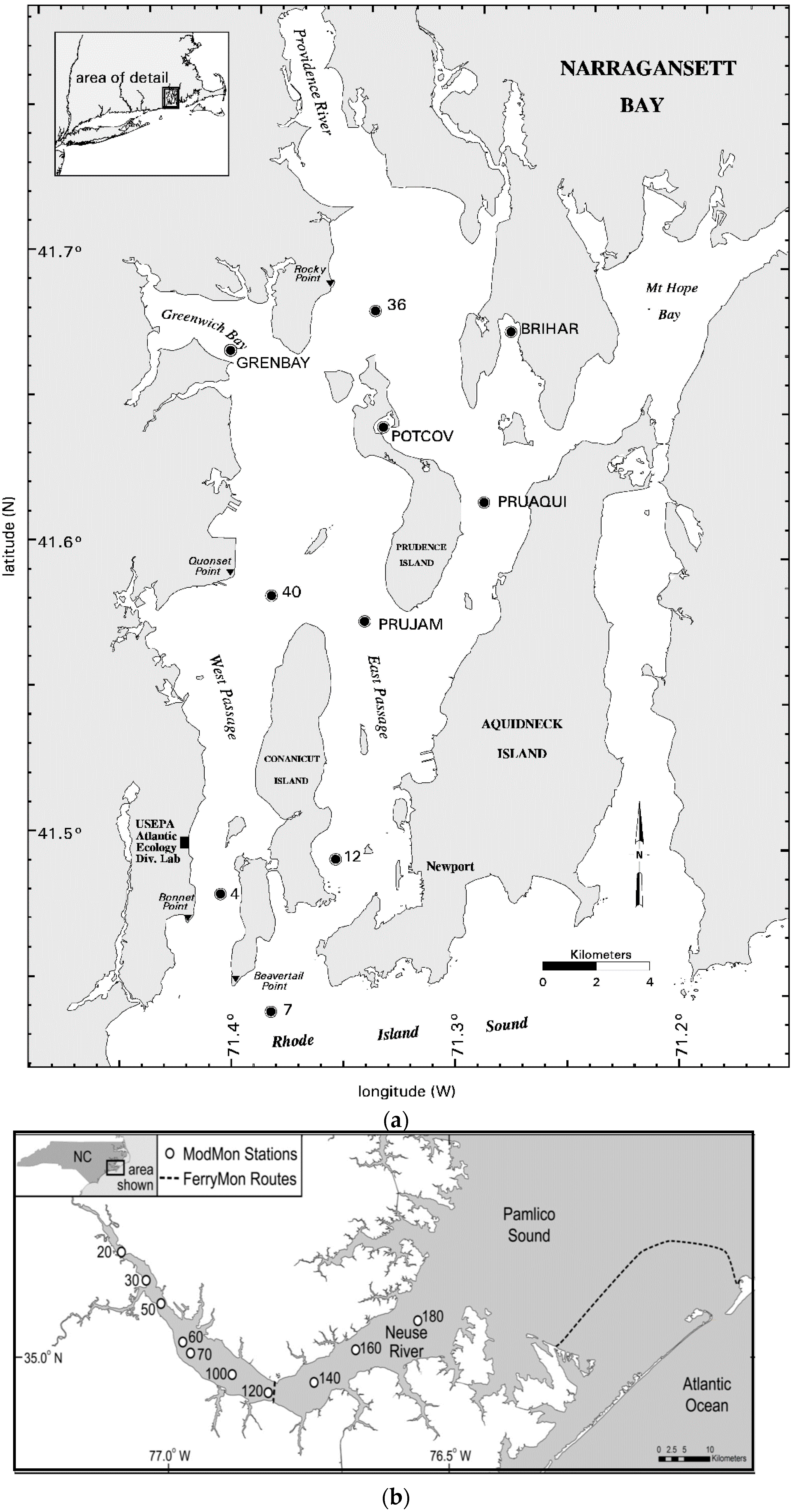
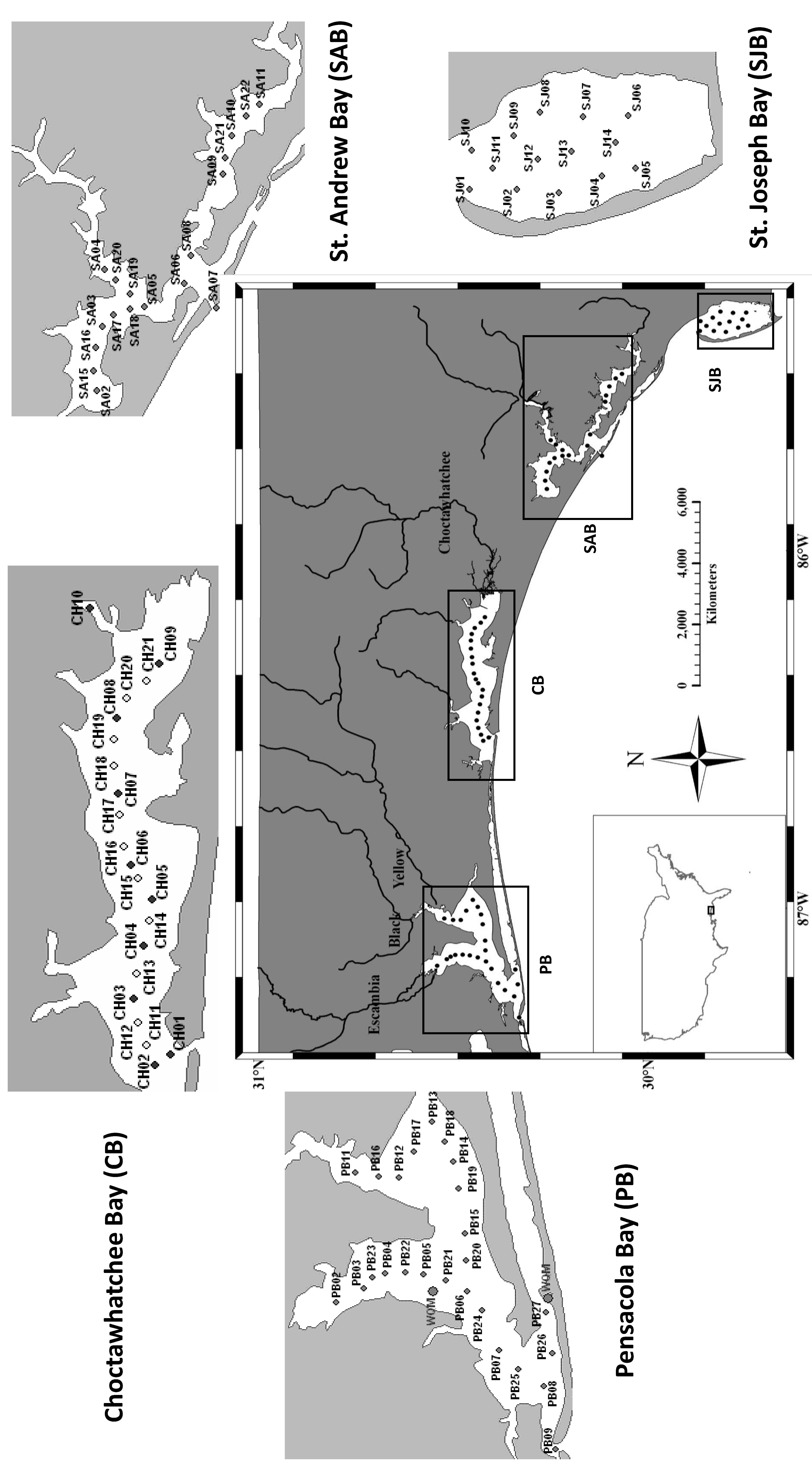
Evaluate these algorithms using in situ radiometric data, laboratory measured CDOM absorption coefficients, and in situ salinity measurements from Narragansett Bay (Rhode Island), New Bedford Harbor (Massachusetts), Neuse River (North Carolina), Pensacola Bay (Florida), Choctawhatchee Bay (Florida), St. Andrews Bay (Florida), St. Joseph Bay (Florida) and Gulf of Mexico inner continental shelf.
(6)
Using regression analysis, validate the performance of the CDOM and salinity algorithms in Pensacola and Choctawhatchee Bays during summer 2011 using match-ups between Hyperspectral Imager for Coastal Ocean (HICO) spectral data, in situ salinity data, and laboratory measured CDOM absorption coefficients from these estuaries.
(7)
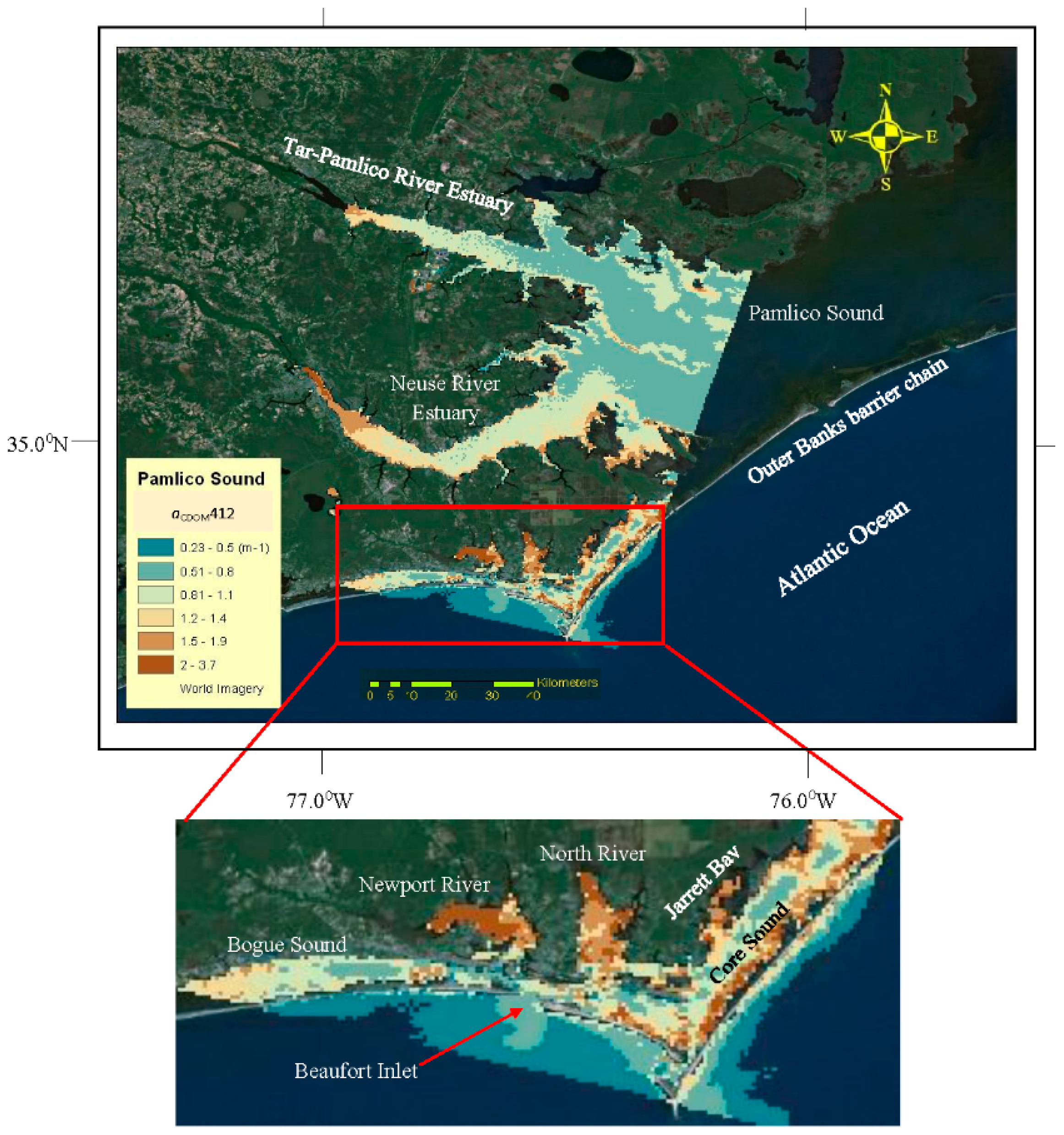
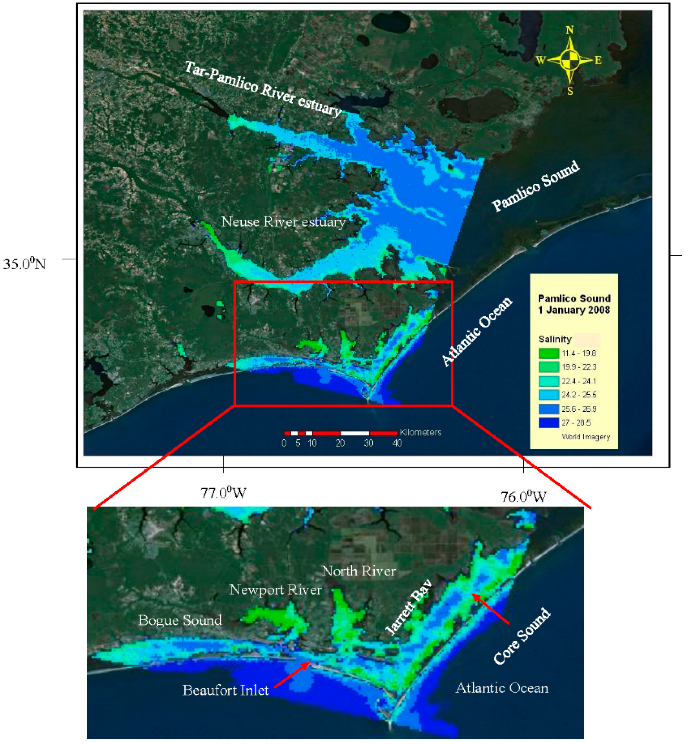
As an example of the applicability of these algorithms to other satellite sensor data, apply the CDOM absorption and salinity algorithms to a full resolution (300 m) Moderate Resolution Imaging Spectrometer (MERIS) image of the Neuse River estuary to illustrate the spatial distribution of CDOM absorptions and surface salinities within one of the most important commercial seafood nurseries along the US East Coast.
The approach that we used here is based on theoretical work of Bowers et al. [33] in which they proposed that a simple band ratio model could be derived to estimate CDOM absorption at 440 nm from the ratio of reflection coefficients (R1/R2). Further, salinity could be derived if the relationship between CDOM absorption and salinity is known. Generally, R1/R2 is a function of absorption (a) by water (w), particulates (p), and yellow substance or CDOM (y) at two bands. By inversion:
R1/R2 = ((aw2 + ap2 + ay2)/aw1 + ap1 + ay1)
If R1 is chosen to be in the red end of the spectrum where CDOM is not absorbed, then ay1 = 0 and
R1/R2 = ((aw2 + ap2 + a*y2 × g440)/aw1 + ap1)
where ay2 is rewritten as is the product of a specific absorption coefficient (a*y2) and g440 is the concentration of CDOM at 440 nm. Solving for g440:
g440 = ((aw1 + ap1)/a*y2)) × R1/R2 − (aw2 + ap2)/a*y2
Bowers et al. [33] suggested that at the red wavelengths, with the exception of very turbid waters or plankton blooms, aw1 > ap1 and therefore aw1 + ap1 ≈ aw1. If R2 is chosen in another location in the spectrum where aw is low, then ap2 > aw2 and ap2 + aw2 ≈ ap2. With this understanding, Equation (3) simplifies to:
g440 = (aw1/a*y2) × (R1/R2) − ap2/a*y2
Bowers et al. [33] further suggested that Equation (4) would predict a linear relationship between g440 and the reflectance ratio when one band is red and the other is another color and that ratio will continue to increase as g440 increased. In theory, the term ap2/a*y2 is a constant that is dependent on light absorption by particulates. However, variations in particulate absorption resulted in variations in the intercept of the linear relationship predicted by Equation (4). Bowers et al. [33] minimized this unwanted effect by selecting an R2 band where a*y2 >> ap2. This meant choosing a band towards the blue end of the spectrum where CDOM absorption is greatest. In this paper, we use the term aCDOM440 instead of g440 to refer to CDOM absorption at 440 nm.
The theory was tested by Binding and Bowers [34]; Bowers et al. [35]; and Bowers et al. [36] which showed that the absorption of light by CDOM in marine waters could be derived using a simple band ratio of Rrs and confirmed that the relationship between CDOM absorption and salinity was inversely related over the salinity range of 15–35 found in estuaries and adjoining coastal seas. Additionally, using a Sea-Viewing Wide Field-of View Sensor (SeaWiFS) image over Northern Europe, Binding and Bowers [35] retrieved CDOM absorption values at 440 nm (aCDOM440) to calculate and map the distribution of salinities from 16 to 34 along the coast and offshore areas of the Clyde Sea, Scotland. However, with a spatial resolution of 1.1 km, the SeaWiFS image was unable to view regions of lower salinity within adjoining lochs and estuaries. Bowers et al. [36] continued to explore the approach of using the linear relationship between in situ aCDOM440 measurements and spectral band ratios to map surface salinities for the Conwy estuary in North Wales, Great Britain.
The bio-optical models presented here to estimate CDOM absorption and surface salinities were derived from several large datasets acquired by the USEPA during surveys of estuaries, coastal bays, and nearshore waters along the U.S. East and Gulf coasts from 1999 to 2012 (referenced by abbreviations found in Table 1).

2. Materials and Methods

Water samples, CTD data, and spectral measurements were collected from all systems from 1999 to 2011 (Figure 1, Table 1). These systems represented a geographically diverse group of water bodies which included meso-tidal, weakly stratified to well mixed, New England estuaries (NB, NBH); a large lagoonal Mid-Atlantic estuarine system (NR); and several partially mixed, microtidal, shallow estuaries characteristic of the northwest coast of the Gulf of Mexico (PB, CB, SAB, and SJB). Sampling stations in all systems were located to characterize water quality and optical properties along the major salinity gradients of each estuary.

2.1. Spectral Measurements

Spectral data were collected to derive Rrs values at stations sampled for water quality and CDOM analysis using multispectral and hyperspectral data acquisition systems.
In NB, optical data were collected at four stations along West Passage and Rhode Island Sound (May 1999–June 2000) using both a Biospherical Instruments multispectral Profiling Reflectance Radiometer (Model PRR 600). From June 2005–July 2007, nine additional stations were sampled in the Providence River, Greenwich Bay, Bristol Harbor, East and West Passages, and Rhode Island Sound (Figure 1a) using a Satlantic HyperPro Profiler II hyperspectral profiling acquisition system. In the NBH, spectral data were also collected at four stations using the Satlantic HyperPro Profiler II system (Freeman [37]; Keith [20]). The Biospherical PRR 600 logged in situ spectral data at 412, 443, 490, 510, 555, 665, and 683 nm. The PRR data were concurrently collected with a surface sensor (Biospherical PRR 610), optimized for in-air use, to measure incident downwelling irradiance (Es) at 412, 443, 490, 510, and 555 nm. The HyperPro Profiler II system was deployed in surface mode (<3 m depth) to acquire spectral measurements of in situ water radiance from 350 to 800 nm. Downwelling irradiance (Ed), from 350 to 800 nm, was measured (in-air) using a shipboard mounted HyperOCR hyperspectral radiometer. In NR, Rrs data were retrieved at stations along the salinity gradient also using a Satlantic HyperPro remote sensing system which logged in-water radiance, sky radiance and downwelling irradiance from 350 to 800 nm (Figure 1b; Sokoletsky et al. [38]). For the Florida estuaries, Rrs was retrieved at stations using the Satlantic HyperSAS system which logged above-water radiance, sky radiance and downwelling irradiance from 350 to 800 nm (Keith et al. [39]. The above-water Rrs spectra were corrected following procedures in Gould et al. [40].
HyperSAS and HyperPro radiance and irradiance data were processed using the Satlantic ProSoft data analysis package. ProSoft is an interactive graphical data processing and extraction application for Satlantic sensors. Data collected by the Biospherical radiometers was processed to obtain Rrs using programs written in Matlab programming language (Appendix 4 in Freeman [37]).

2.2. Determination of CDOM Absorption Coefficients

In NB, surface water samples (~0.5 m depth, n = 92) were collected to derive CDOM absorption coefficients at four stations along the West Passage and Rhode Island Sound (May 1999–June 2000) and nine additional stations (June 2005–July 2007) in the Providence River, Greenwich Bay, Bristol Harbor, East and West Passages, and Rhode Island Sound (Figure 1a). Samples were also collected at four stations (n = 4) in the NBH during June 2005. CDOM absorption coefficients, were expressed in units of per meter (m−1) as a measure of how far into the water column light was able to penetrate before it was absorbed.
NB and NBH samples were placed on ice in the field for later transport for laboratory analysis. In the laboratory, water for CDOM absorption analysis was twice filtered using 47 mm Millipore filters (nominal pore size = 0.2 μm) to remove small particles and colloids. Absorption coefficients were determined from measurements of the optical density (OD) of the water samples over the spectral range of 400–700 nm using Perkin Elmer Lambda 3 Double-Beam UV-Visible (samples collected between 1999 and 2000) and Perkin Elmer Lambda 35 Double-Beam UV-Visible (samples collected after 2000) Spectrophotometers with a spectral resolution of 0.5 nm using 10 cm path length cells (Bricaud et al. [41]; Mitchell et al. [42]; Keith et al. [19]). The OD was determined using:
OD = log10(I0/I)
where I0 is the absorbance of the water sample and I is the absorbance of a reference sample, in this case deionized water. CDOM absorption was calculated using:
a(λ) = 2.303 × [(ODs(λ) − (ODb(λ))/l]
where ODs(λ) = sample absorbance, ODb(λ) = sample blank absorbance, and l = cuvette pathlength.
Absorption coefficients were corrected for backscattering of small particles and colloids not removed during filtering according to Bricaud et al. [42]. Salinity measurements were also made at each NB and NBH station using a Seabird Sealogger CTD SBE 25 profiler lowered to the same depth as the water samples and the data averaged from the surface to depth (Keith et al. [19]; Keith [20]).
In NR, surface water samples (~1 m depth, n = 74) were collected from October 2006–October 2008 at 10 sampling sites (Figure 1b). Salinity and CDOM data were obtained as part of the Neuse River Estuary Modeling and Monitoring Project (ModMon), which is a collaborative effort between the University of North Carolina-Chapel Hill and the NC Department of Environment and Natural Resources and the North Carolina Department of Transportation Ferry-based Monitoring (FerryMon) Program. Water temperature, salinity, dissolved oxygen, chlorophyll fluorescence, and turbidity were collected with each crossing of the Neuse River and Pamlico Sound by FerryMon using flow-through YSI 6600 sondes.
For PB and the other Florida estuaries, surface water samples (~1 m depth, n = 87) were collected from four locations from April 2010 and June 2011–June 2012 (Figure 1c). CDOM absorption coefficients were determined using water filtered through Whatman 47 mm GF/F glass fiber filters (nominal pore size = 0.7 μm) and absorbance was measured using a 10 cm cuvette with a Shimadazu UV1700 dual-beam spectrophotometer (Schaeffer et al. [43]). OD and absorption coefficients were derived using Equations (1) and (2). Data were collected at 1 nm intervals between 200 and 750 nm. Spectra were normalized for backscattering of small particles and colloids using Pegau et al. [44]. Salinity was concurrently measured at each station using a Seabird 25 SBE CTD system (Keith et al. [39]).

2.3. CDOM Algorithm Development

Historically, CDOM absorption at 440 nm (aCDOM440) has been used as the parameter to indicate the concentration of CDOM in marine and fresh waters. This wavelength was chosen because it approximately corresponds to the mid-point of the blue waveband peak that most classes of algae have in their photosynthetic action spectrum (Kirk [45]).
In this study, laboratory measured CDOM absorptions at 412 nm (aCDOM412) and aCDOM440 values were regressed against CTD measured salinities (n = 176) obtained from NB (1999–2000, 2003), NR (2006–2008) and SAB (2010) to determine wavelength choice for inclusion into the CDOM algorithm development process. Wavelength selection was based on the strength of the relationships for each wavelength as derived from scatterplots.
Once a wavelength was chosen, the CDOM absorption model was derived from linear regression of Rrs ratio of 665 and 490 nm against laboratory measured CDOM absorptions at the wavelength identified from NB (1999–2000 and 2005–2007) and NR (2006–2007). The CDOM spectral model was validated using a subset of spectral and laboratory data not used during model creation.
As part of the development process, scatterplots were created to illustrate the relationship between predicted and measured absorption values. The Major Axis method of Model II linear regression was used, not to develop a predictive relationship between the variables as in Model I regression analysis, but to examine functional relationships between predicted and measured absorption values (Laws [46]). The strength of the relationships was determined from the goodness of fit (R2) of the values and slope (m) of the regression. The statistical significance of the regression is expressed by its p-value. The measurement uncertainty for all algorithms derived in this study was calculated as the root-mean-square error (RSME) and the percentage root-mean-square error (%RSME), using:
RMSE = 1 n * ( a C D O M 412   m e a s u r e d a C D O M 412   p r e d i c t e d ) 2
where n = number of samples.
The %RMSE was determined using:
% RMSE = 1 n * ( a C D O M 412   m e a s u r e d a C D O M 412   p r e d i c t e d ) 2 * 100 *   n a C D O M 412 m e a s u r e d

2.4. Salinity Model Development

Following a procedure similar to the development of the CDOM absorption model, the salinity algorithm was derived from linear regression of surface salinities (ranging from S < 5 to S > 20) against measured aCDOM412 values from NB (1999–2000), NR (2006–2008) and PB (2009–2010). The model was validated using a subset of spectral and laboratory data not used during model creation collected from NB (1999–2000 and 2003–2005), NR (2006–2007), SAB (2011), SJB (2011), CB (2009–2011) and PB (2010–2011) as well as published literature values from the northwestern Gulf of Mexico inner continental shelf (D’ Sa and DiMarco [47]; Tehrani et al. [27]).
A scatter diagram of between predicted and measured salinity values was produced to explore the relationship indicated by the data. Using Model II linear regression analysis, the strength of the relationship was determined from the R2 of the values and the slope of the regression line (Laws [47]). The uncertainty associated with the model was determined from the RMSE.

2.5. Validation of CDOM and Salinity Algorithm Performance

We used hyperspectral data from HICO to derive estimates of aCDOM412 and salinity. These values were compared with in situ optical data and CDOM absorption coefficients from the Gulf coast estuaries to determine algorithm performance. Validation match-ups used data from inland brackish water environments as well as coastal locations to measure the performance of the CDOM and salinity algorithms. HICO images were previously acquired from Oregon State University as radiometrically calibrated Level 1B top-of-atmosphere (TOA) at-sensor radiances. These images were processed using EXELIS ENVI version 4.7 software to retrieve Rrs values (Keith et al. [39]). During processing, each image was atmospherically corrected using the dark pixel subtraction method to remove atmospheric effects (Keith et al. [39]; Tufillaro et al. [48]; Chavez [49]). The Rrs values retrieved from image processing were used in the algorithms to create scatterplots of measured and predicted values. Using Model II linear regression analysis, the strength of the relationships between these observations was determined from the R2 values and the slope of the regression line.

2.6. Application Example

A MERIS image was used as an example to show the portability of the validated algorithms when applied to a multispectral data product to predict and map the distribution of CDOM absorptions and salinities in a U.S. East coast estuary. For this example, radiometrically calibrated and atmospherically-corrected, full resolution (300 m pixel size) Level 2 top-of-atmosphere (TOA) at-sensor radiances were acquired from the European Space Agency, and atmospherically corrected according to Sokoletsky et al. [38].

3. Results

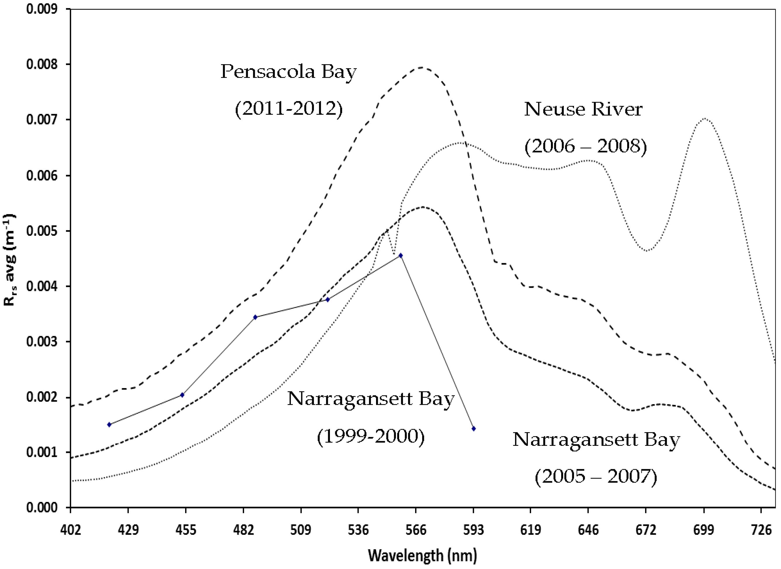
3.1. Spectral Measurements

Coastal and estuarine waters are considered to be optically complex because CDOM and mineral particles can make a significant contribution to water color and brightness. The average remote sensing reflectance curves are presented for NB, NR and PB (Figure 2). Results indicated that these estuaries are spectrally similar with reflectance curves that are characteristic of coastal and estuarine waters. All curves showed low reflectances in the blue end of the spectrum due to light absorption by CDOM, suspended matter, and phytoplankton pigments and reflectance peaks around 550 nm due to detrital backscatter. While NB and PB have very similar curves, the higher reflectances of the PB curve around 550 nm indicated these estuarine waters are more turbid relative to the New England counterpart. In comparison, NR showed low reflectances, similar to NB and PB, in the blue end of the spectrum but elevated reflectances between 550 and 660 nm which are a function of high turbidity. A large phytoplankton reflectance peak in the red and near infrared portion of the spectrum near 700 nm indicated high chl a concentrations.

3.2. Determination of CDOM Absorption Coefficients

Regression analysis of in situ salinities from NB, NR and SJB against laboratory measurements of aCDOM412 and aCDOM440 from concurrently collected water samples showed that aCDOM412 had a higher goodness of fit (R2 = 0.92) than aCDOM440 (R2 = 0.67) (Figure 3). The increased scatter in the aCDOM440 scatterplot corresponded to salinities and water samples from NR and SJB which are characterized by salinities less than 20 and high CDOM absorption values. The high R2 of the aCDOM412 scatterplot indicated a better correlation with salinities over the range of <5 to greater than 30 S and CDOM absorptions <1 to ~7 m−1. Therefore, in this study aCDOM412 was chosen as the wavelength to use for retrieving salinities using satellite data from near coastal and estuarine waters along the US East and Gulf coasts.

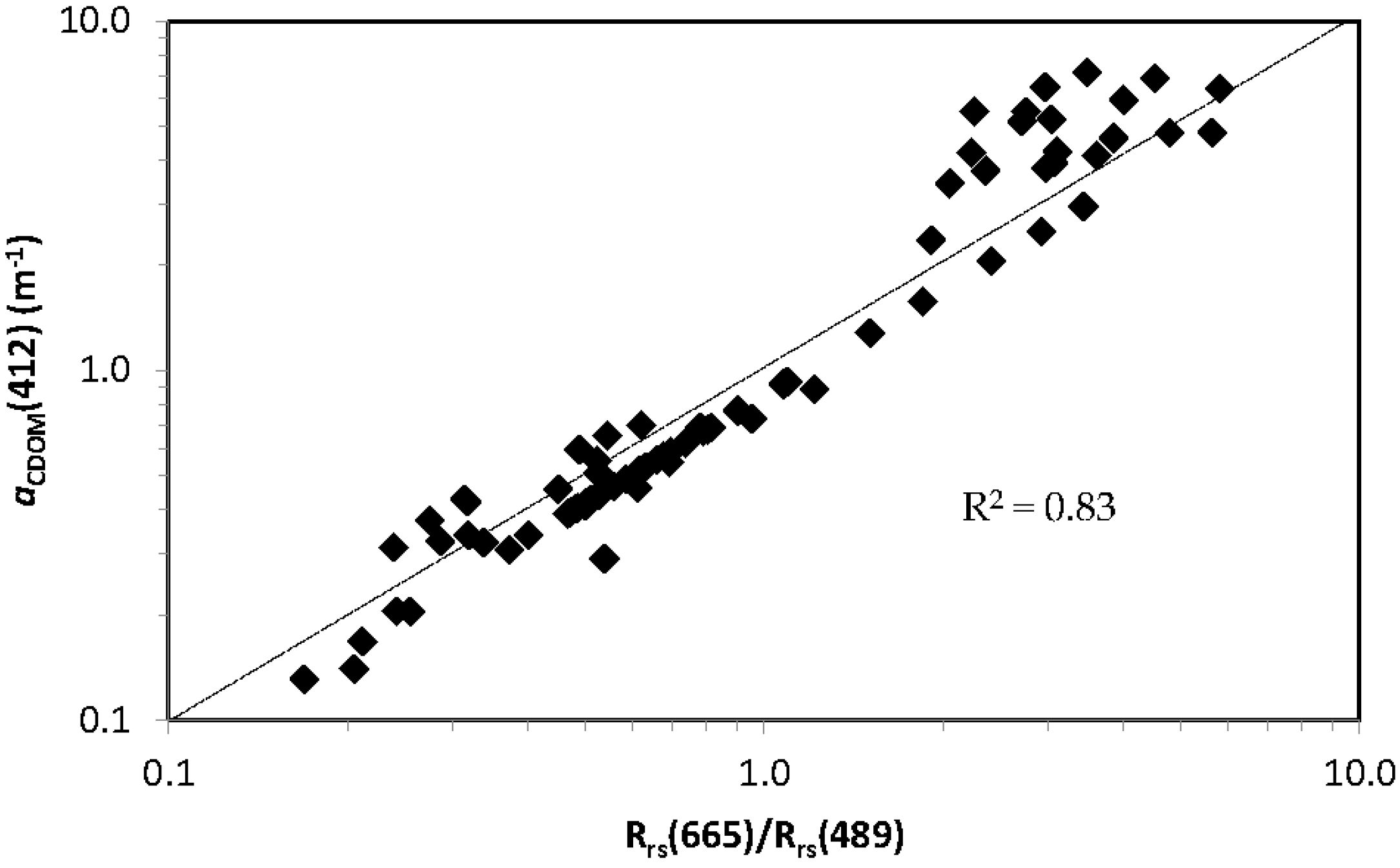
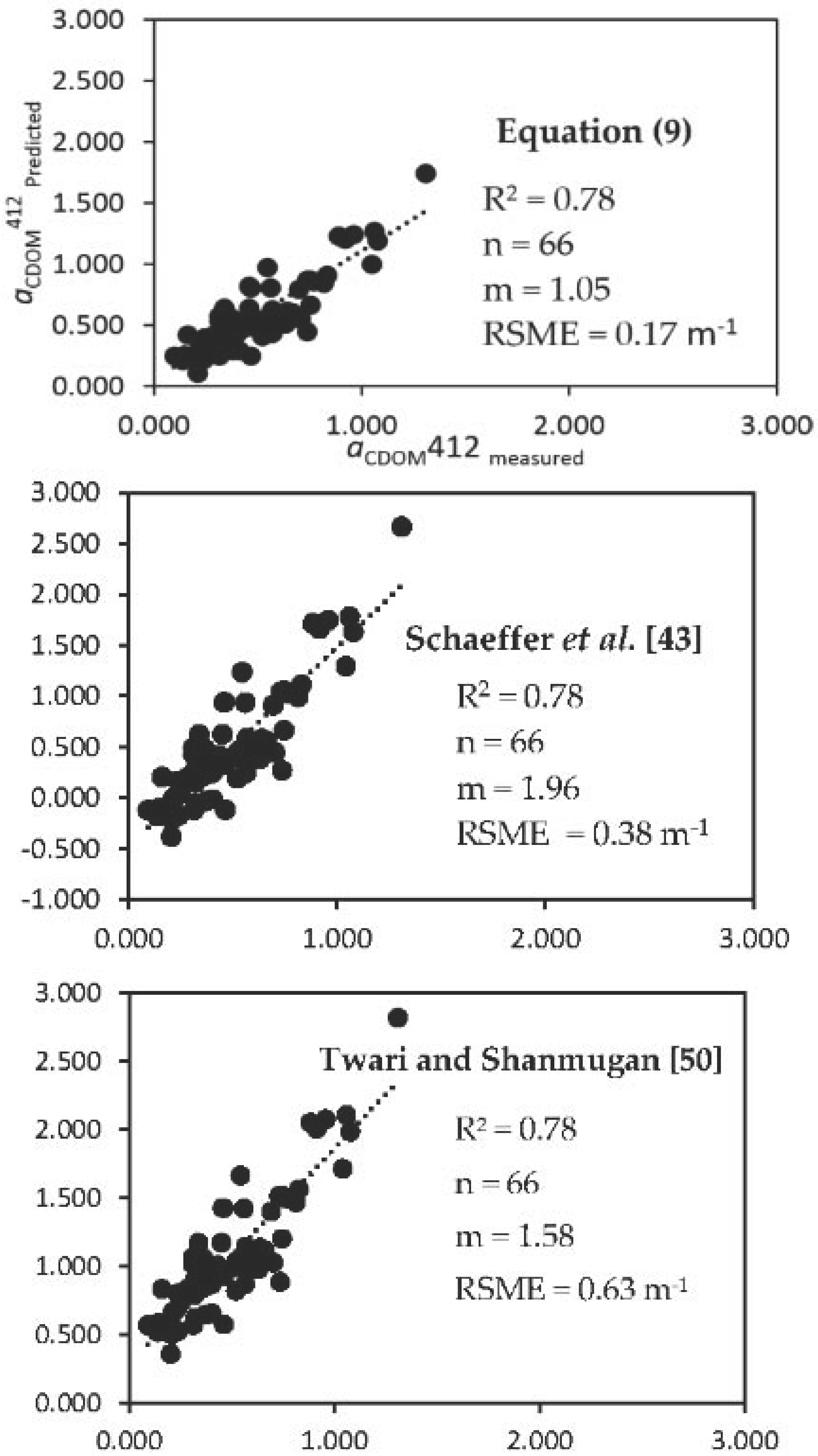
3.3. CDOM Absorption Algorithm

To predict the CDOM absorption coefficients from coastal and estuarine water color, in situ and above-water remotely sensed reflectances at 665 and 490 nm were regressed against laboratory derived absorption values at 412 nm to predict aCDOM412 over the entire absorption range found in our study areas (Figure 4, Table 2). Using laboratory measured CDOM absorption values and concurrently acquired in situ spectral data from NB, NR, NBH, SJB, and PB (Table 1) the following equation was derived for application to nearshore marine and estuarine environments.
aCDOM412 = 1.3499 × (Rrs665/Rrs489) − 0.1124
Comparisons between measured CDOM absorption values and the ratio of Rrs values at 665 and 490 nm showed an excellent relationship (R2 = 0.83; Figure 4). Results from Model II linear regression analysis indicated robust correlations (r = 0.97) for absorption values <7 m−1 and a strong goodness of fit (R2 = 0.95) between measured absorptions and those predicted by the algorithm, and a %RMSE = 29.4 (Table 3; Figure 5).

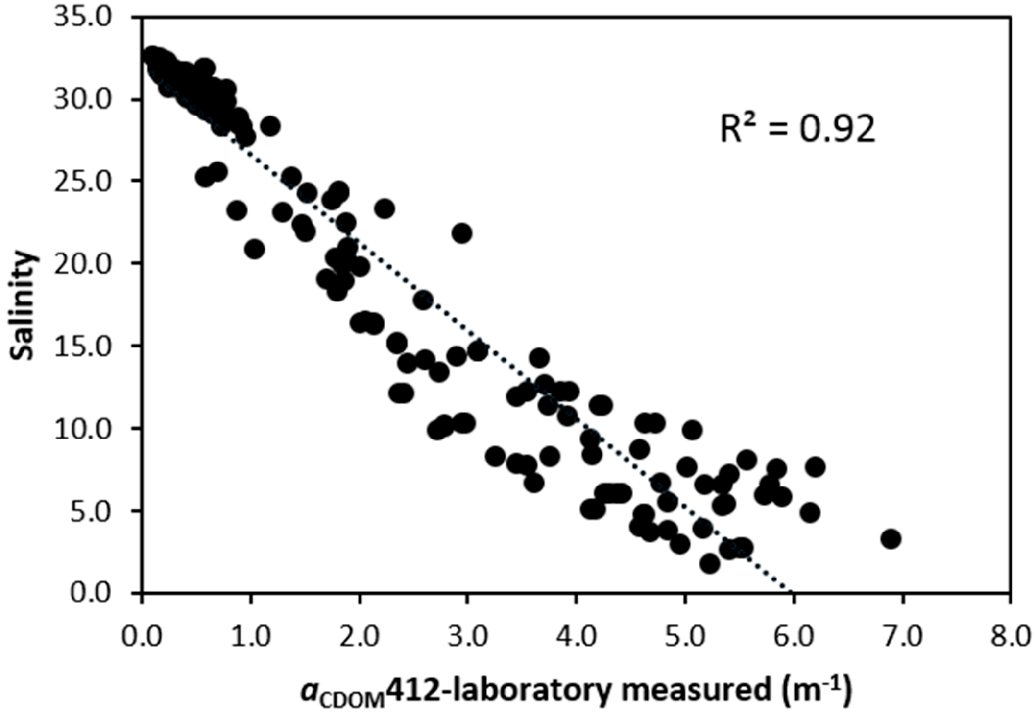
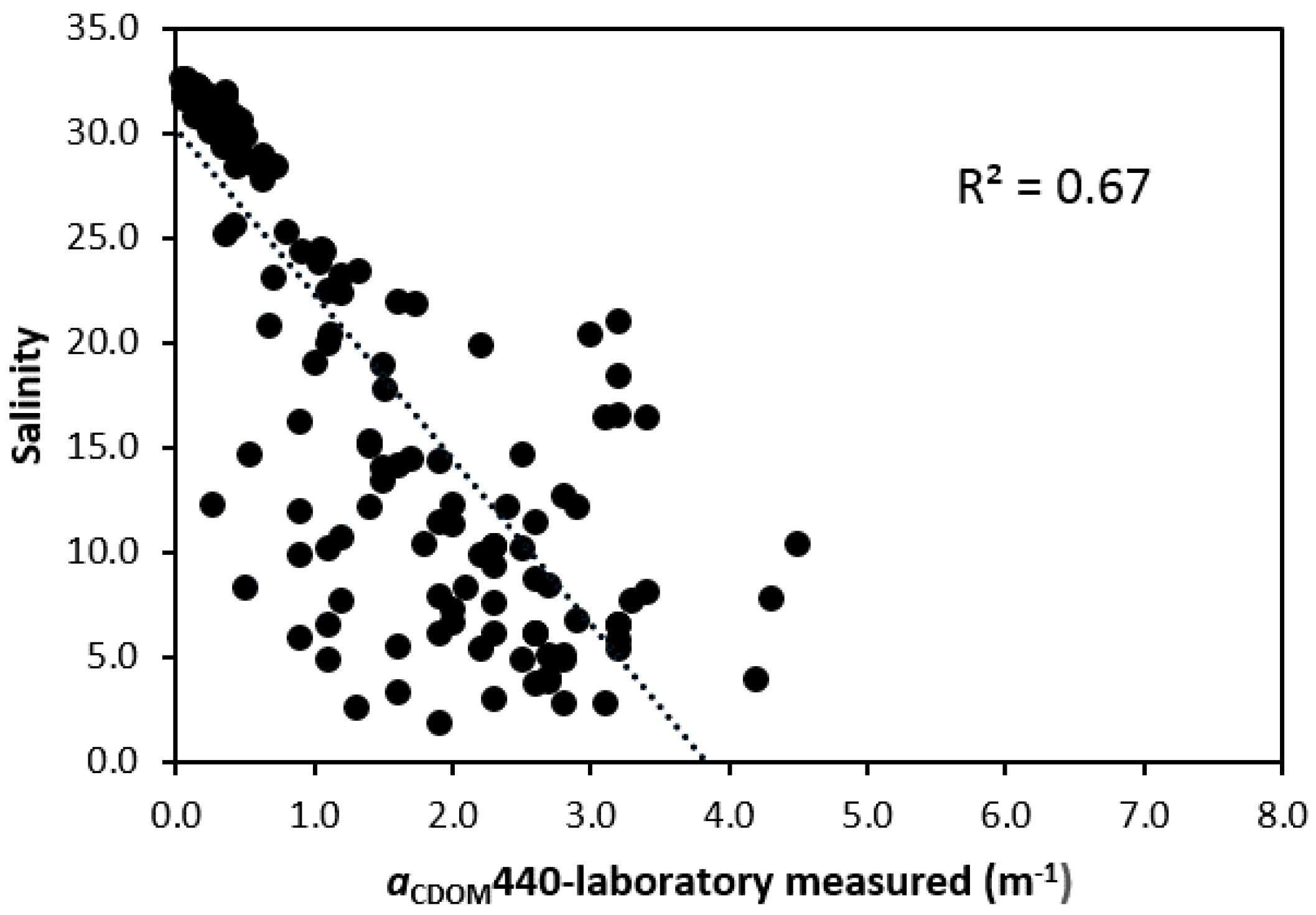
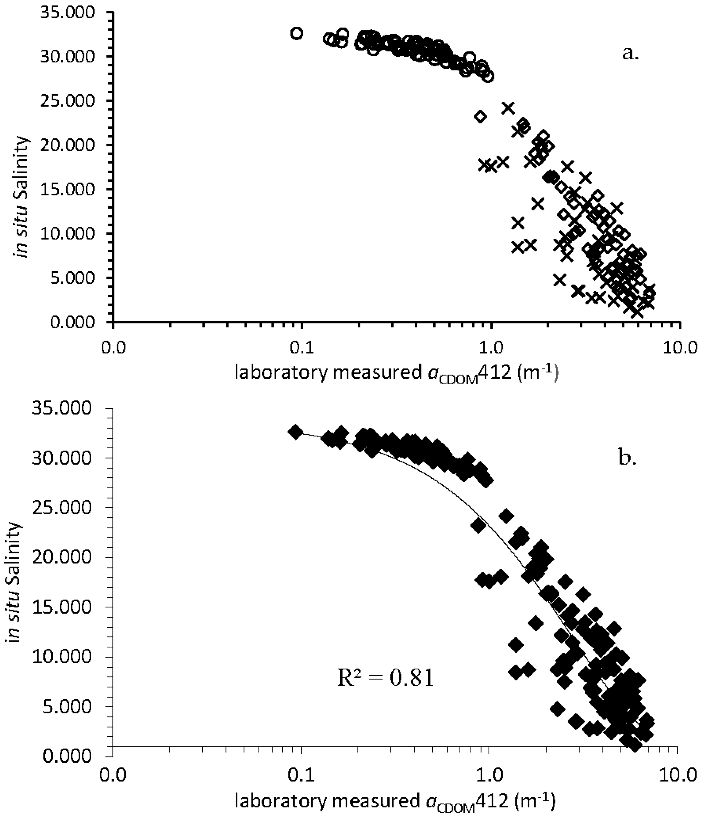
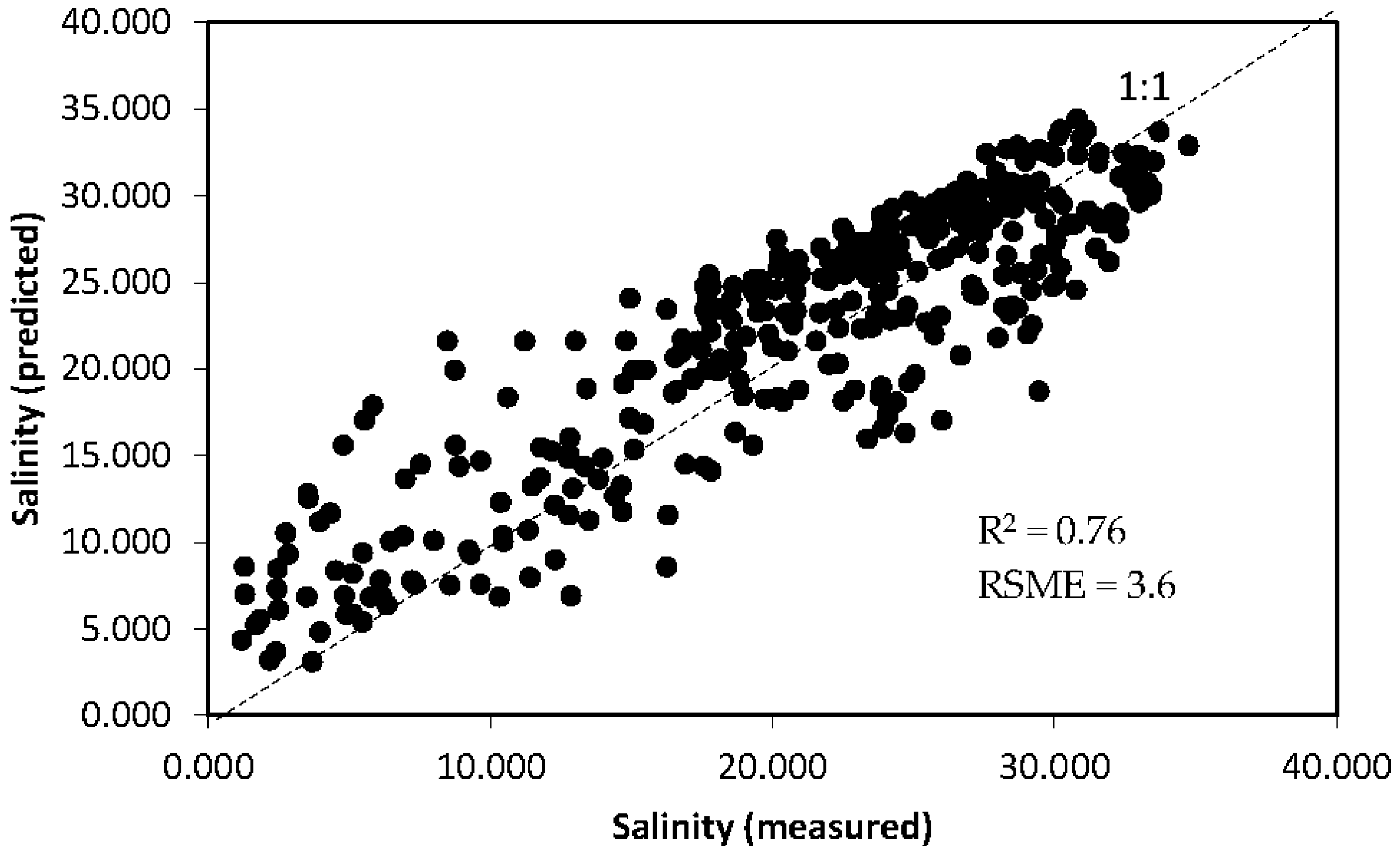
3.4. Salinity Algorithm

The following equation was derived from locations in the NB, NR, and PB (Table 1):
Salinity = 33.686 × exp (−0.374 × aCDOM412)
Results showed an excellent relationship (R2 = 0.81) between measured CDOM absorption and measured salinities (Figure 6a,b, Table 2). Results from Model II linear regression analysis indicated a strong goodness of fit (R2 = 0.76) between measured and predicted salinities, an RSME for S = 3.6 and %RMSE for S = 15.9 (Figure 7; Table 3).

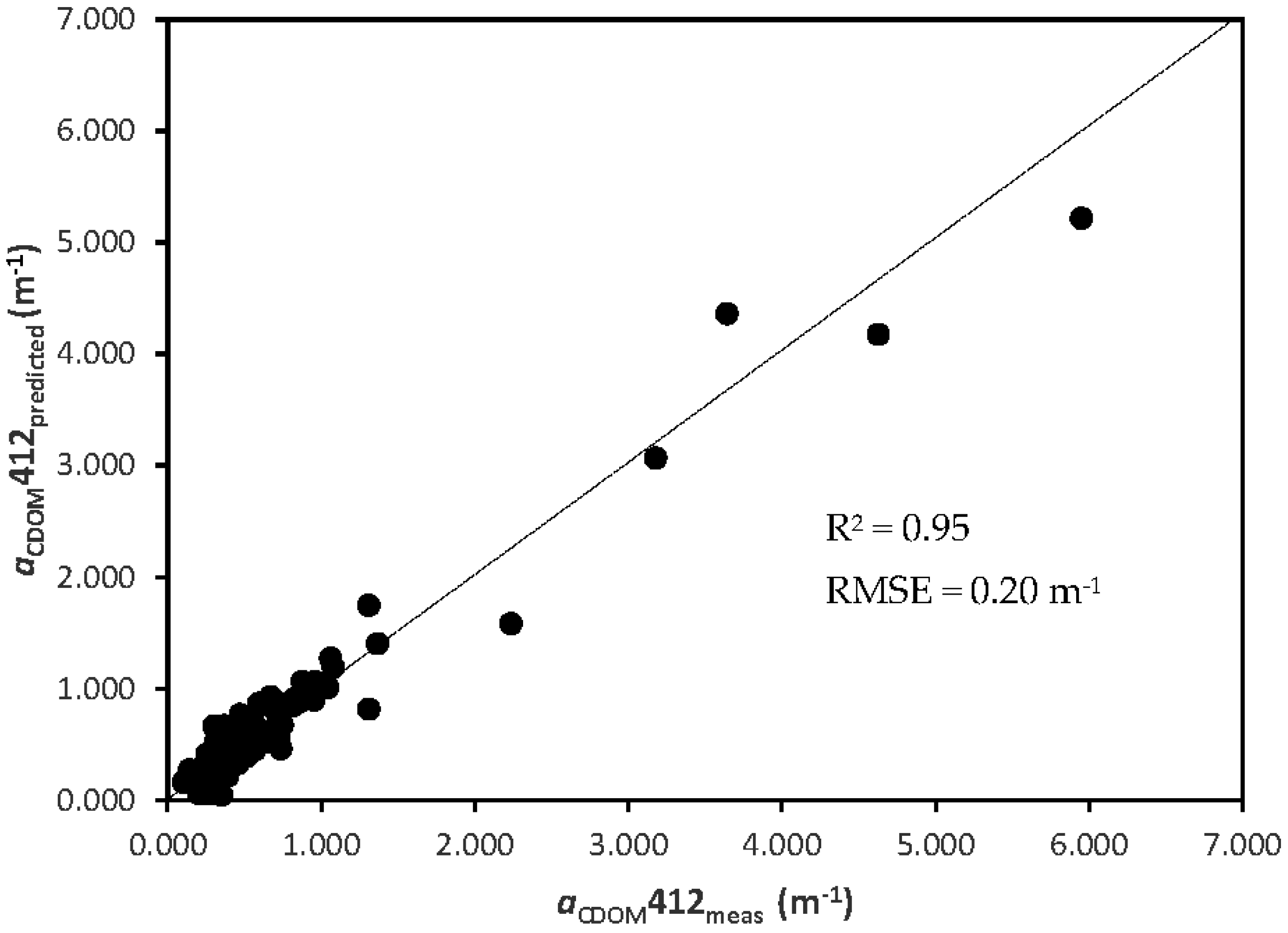
3.5. Validation of CDOM and Salinity Algorithm Performance

Using in situ Rrs665/Rrs490 and laboratory measured CDOM absorption values from NB (1999–2000), SJB (2010), and PB (2011), comparisons were made between aCDOM412 values derived from Equation (5) and aCDOM412 values derived from algorithms in Schaeffer et al. [43] and Twari and Shanmugam [50] to validate algorithm performance. Both studies used the red to blue-green spectral band approach to estimate CDOM absorption (Table 4). Results indicated that the goodnesss of fit was the same (R2 = 0.78) for all three models, however Equation (9) results had the lowest %RMSE (34.9%) when compared to %RSME values derived from results produced by the and Schaeffer et al. [43] (84.4%) and Twari and Shanmugam (118%) algorithms (Figure 8). Equation (9) also had a slope (1.1) closest to unity when compared with Twari and Shanmugam (1.6) and Schaeffer et al. [43] (2.0) (Table 5).
Hyperspectral data from HICO were also used in both algorithms to generate sensor-derived aCDOM412 and salinity products for validation. There are only a few match-ups available for validating these products because of limited number of overflights of the northern Gulf of Mexico and coincident data sets of in situ spectral and field measurements. Atmospherically corrected images were acquired on 2 June, 30 July, and 9 September 2011 from the lagoonal, brackish waters of PB and CB for CDOM match-ups (Keith et al. [39]). HICO images were acquired on 2 June and 30 July 2011, and 14 April 2010 from PB, CB, and SAB for salinity match-ups (Keith et al. [39]).
For the CDOM and salinity match-ups, data collected within 5 h after a HICO over flight were used for the validation. Model II linear regression of validation match-ups for CDOM absorption showed an excellent correspondence between HICO-derived aCDOM412 versus measured aCDOM412 absorptions (R2 = 0.93; Figure 9a) and a slope of 1.4 (Table 6). RMSE analysis of predicted versus measured absorptions resulted in an uncertainty of 0.84 m−1 (Table 6).
The salinity validation match-ups showed a strong correlation between HICO-derived salinities versus in situ salinities (Figure 9b). RMSE analysis of predicted versus measured salinities resulted in an uncertainty of 3.3 (%RMSE = 15.7%; Table 6). Model II linear regression of measured values and those derived from HICO yielded an R2 = 0.70 and a slope of 1.27 (Table 6). Possible causes of discrepancies observed between the HICO retrievals and the in situ data could be due to uncertainties with the algorithms, sub-pixel heterogeneities in the images, and temporal differences in water sampling, tidal phase, and sensor overflight.

3.6. Application Example

Spectral data retrieved from a full resolution (300 m pixel size) MERIS image (1 January 2008) of the Pamlico Sound (NC) estuary system were applied to Equations (5) and (6) to illustrate how multispectral data can be transformed into maps to illustrate CDOM absorption and salinity variability on large and fine spatial scales in a coastal setting (Figure 10 and Figure 11). The satellite-based imagery clearly illustrates that the highest aCDOM412 values (1.5–3.7 m−1) occurred in the uppermost regions of the larger Neuse and Pamlico River estuaries, smaller estuaries (Newport and North Rivers) and Jarrett Bay along the southern coastline (Figure 10). Values decreased (~1.9–1.2 m−1) along the middle reaches of the Neuse and Tar-Pamlico River systems due to mixing of freshwaters with the more saline waters of Pamlico Sound. Inshore of the Outer Banks barrier island system, high absorption values (~3.7–1.5 m−1) are associated with freshwater drainage from emergent wetland complexes. In Core Sound, values ranged from 0.8 m−1 in the middle of the bay to 1.4 m−1 along adjoining coasts. An east to west absorption gradient (from ~1.2–0.8 m−1) occurred along Bogue Sound as coastal ocean water mixed with brackish bay waters. Lowest absorption values (~0.23–0.5 m−1) were characteristic of the more saline waters of the Atlantic Ocean (Figure 10). The 300 m pixel resolution of the MERIS image also made it possible to observe the transport of dissolved organic matter through Beaufort Inlet along the south shore into the Atlantic Ocean (Figure 10 inset).
The CDOM product was transformed into a map of the spatial distribution of salinity in the MERIS image (Figure 11). Characteristically, the lowest salinities (S = 11.4 to 19.8) are associated with areas of highest CDOM absorption in the Newport and North River estuaries and in Jarrett Bay (Figure 11 inset). Salinities increased inversely as CDOM absorption decreased (e.g., Bogue Sound) with highest salinities (S = 25.6–26.9) occurring in Pamlico Sound, in the middle of Core Sound (Figure 10 insert) and in the coastal Atlantic Ocean (S = 27–28.5) (Figure 11).

4. Discussion

In order to determine the absorption coefficients needed for developing the CDOM and salinity algorithms, water samples were collected in several estuaries by USEPA field programs and analyzed in laboratory settings according to published, standardized operating procedures. As a part of these protocols, water samples collected from the estuaries in this study were routinely filtered using 0.22 μm Millipore filters or Whatman GF/F 0.7 μm filters. The use of these different pore sizes has raised discussions concerning the comparability of absorption data from the sampled estuaries. A study by Ferrari and Tassan [51] directly addressed any concerns by comparing the use of Whatman GF/F 0.7 μm and Millipore 0.22 μm filters for chlorophyll, particle, and absorption measurements. Their study found no statistical difference between these filter types and concluded that performance of both filters to be comparable.
We also investigated which wavelength was appropriate, either 412 or 440 nm, for estimating salinity from CDOM absorption in near coastal and estuarine waters along the US East and Gulf coasts. As presented earlier, aCDOM440 was the wavelength of choice of several remote sensing studies in ocean and nearshore waters. This selection was supported by results obtained by the Ocean Physics Laboratory during the HyCODE 2000 experiment which showed that aCDOM440 was the only property of the bio-optical and oceanographic parameters measured (e.g., chl a concentration, aCDOM440, total particle scattering and total light attenuation) along the New Jersey continental shelf that had a significant relationship with salinity (R2 = 0.78; Coble et al. [4]). However, a search of the scientific literature has also revealed studies that indicated a high correlation existed between in situ salinities and laboratory measured CDOM absorptions towards UV-blue wavelengths (e.g., 355, 400, 412 nm) in Chesapeake Bay, the Gulf of Mexico, Clyde Sea, and the East China Sea (Haltrin et al. [52]; Bowers et al. [33]; Ahn et al. [53]; D’Sa and DiMarco [47]; Du et al. [54]; Tehrani et al. [27]; Bai et al. [55]). In this study, aCDOM412 was chosen as the absorption wavelength for development of the salinity algorithm based on the strong statistical relationship between measured CDOM absorptions at 412 nm and measured salinities in the sampled estuaries. This selection is also appropriate because 412 nm which is one of the more commonly found wavelengths in ocean color satellite sensor data.
The relationship between laboratory measured CDOM absorption values at 412 nm and in situ salinities showed that, in general, the inverse relationship observed in previous studies was robust across the range of coastal environments in this study. Results showed that salinities exponentially decreased as CDOM absorption increased from salinities ranging from S = 2–33. The relationship also appeared to consist of two trends that may be related to freshwater input and mixing processes characteristic of New England, Mid-Atlantic, and Gulf coast estuaries (Figure 6a). The first trend consisted of a cluster of data points, between S = 28–3, representative of the low freshwater input into NB from adjoining watersheds. The second trend consisted of an increase in the scatter as salinity decreased and CDOM absorption increased in response to increased freshwater input to coastal and estuarine waters in the mesohaline and oligohaline environments of the NR and northern Gulf Coast estuaries and shelf areas. Using these relationships, we selected spectral data from several overflights of Pensacola Bay (Florida) by the Hyperspectral Imager for the Coastal Ocean (HICO) for algorithm validation purposes. Results showed that the salinity model had a strong fit between measured and predicted values (R2 = 0.70) and low error in estimation (RSME ± 3.3) relative to the range of surface salinities (~1.0 to 33.0) observed from CTD data. The CDOM model had an excellent fit between measured and predicted values (R2 = 0.93) and low uncertainty (RMSE ± 0.84 m−1) relative to the range of absorptions (0.1 to ~7 m−1) observed in the laboratory data.
To illustrate the coastal dynamics that can be observed from spectral data when applied to the algorithms, we selected a Medium Resolution Imaging Spectrometer (MERIS) of the Neuse River estuary (North Carolina). Generally, the distribution of CDOM and salinities derived from MERIS imagery of the Neuse River estuary followed the inverse relationship characteristic of these properties in coastal waters. Predicted CDOM distributions made it possible to observe the transport of dissolved organic matter from adjoining watersheds into local waters and through coastal inlets into the Atlantic Ocean. Salinities increased as CDOM absorption decreased.
While the HICO and MERIS sensors are no longer operational, these sensors have provided a wealth of legacy ocean color images for examination and study. For almost a decade, the coastal remote sensing community has relied heavily on MERIS and Moderate Imaging Spectroradiometer (MODIS) multispectral sensors to understand coastal dynamics and processes. However, the 1000 m spatial resolution of MODIS color bands is too coarse to observe the spectral character of most estuaries and bays. MERIS (300 m resolution) and HICO (95 m resolution), the first spaceborne imaging spectrometer designed to sample estuaries and the coastal ocean, were ideally suited for environmental monitoring and algorithm development in estuaries and coastal bays.

5. Conclusions

Using a simple band ratio approach, algorithms were derived for use with estuarine and ocean color data to retrieve accurate estimates of surface CDOM absorption and salinity values in estuarine waters which are often below the pixel resolution of sensors on ocean color satellites. When hyperspectral and multispectral spectral data from HICO and MERIS, respectively, were applied to these algorithms, the resulting products showed strong spatial gradients in CDOM absorption and salinity distribution which were consistent with observed patterns as freshwater/brackish waters are transported from inland systems to the coastal ocean. These models were successfully validated against published algorithms which were also based on the band ratio approach. Within an environmental monitoring context, the data produced by these models, when mapped over scales and long time periods, could illustrate and resolve the response of estuarine systems to increasing freshwater runoff from surrounding watersheds due to anthropogenic activities and climatic events. This study is unique because we have used in situ spectral and field data as well as laboratory analyses from hundreds of samples collected over a twelve year time period to derive a set of algorithms which are optimized for the range of absorptions and salinities characteristic of estuaries along the US East and Gulf coasts. Although the performance of the algorithms was relatively stable along both the East and Gulf coastal estuaries studied, additional research is needed to further evaluate performance for extended geographical applications.

Acknowledgments

Although the research described in this manuscript has been funded by the U.S. Environmental Protection Agency, it has not been subjected to Agency review. Therefore, it does not necessarily reflect the views of the Agency. Mention of trade names or commercial products does not constitute endorsement or recommendation for use. This manuscript is ORD tracking number ORD-014966. The authors declare no conflict of interest. Ross S. Lunetta (USEPA) and Blake A. Schaeffer (USEPA) provided field and laboratory data for the Neuse River (NC) and northwest Gulf of Mexico estuaries. Darryl J. Keith wrote the paper with significant input from Ross S. Lunetta and Blake A. Schaeffer and provided field and laboratory data for the Narragansett Bay estuary. We would like to thank Wayne Munns and Timothy Gleason (USEPA-Atlantic Ecology Division (AED)), Glen Thursby (USEPA-AED), Joseph LiVolsi (USEPA-AED), Jason Grear (USEPA-AED) and four anonymous reviewers for valuable comments and observations during manuscript preparation and revision. A special thanks is given to Doug Levin at the Center for Environment and Society (Washington College) for his comments and insight.

Author Contributions

Darryl Keith, Ross Lunetta, and Blake Schaeffer designed and implemented the field and data collection programs in this study; Ross Lunetta and Blake Schaeffer provided the data from North Carolina and Florida estuaries to Darryl Keith for analysis and model development. Darryl Keith wrote the paper.

Conflicts of Interest

The authors declare no conflict of interest.

References

  1. Zhang, Y.; Yin, Y.; Feng, L.; Zhu, G.; Shi, Z.; Liu, X.; Zhang, Y. Characterizing chromophoric dissolved organic matter in Lake Tianmuhu and its catchment basin using excitation-emission matrix fluorescence and parallel factor analysis. Water Res. 2011, 45, 5110–5122. [Google Scholar] [CrossRef] [PubMed]
  2. Heyes, A.; Miller, C.; Mason, R. Mercury and methylmercury in Hudson River sediment: Impact of tidal resuspension and methylation. Mar. Chem. 2004, 90, 75–89. [Google Scholar] [CrossRef]
  3. Opsahl, S.; Benner, R. Distribution and cycling of terrigenous dissolved organic matter in the ocean. Nature 1997, 386, 480–482. [Google Scholar] [CrossRef]
  4. Coble, P.; Hu, C.; Gould, R.W., Jr.; Chang, G.; Wood, A.M. Colored dissolved matter in the coastal ocean—An optical tool for coastal environmental assessment and management. Oceanography 2004, 17, 50–59. [Google Scholar] [CrossRef]
  5. Del Vecchio, R.; Blough, N. Spatial and seasonal distribution of chromophoric dissolved organic matter ABD dissolved organic carbon in the Middle Atlantic Bight. Mar. Chem. 2004, 66, 35–51. [Google Scholar]
  6. Vodacek, A.; Blough, N.V.; DeGrandpre, M.D.; Peltzer, E.T.; Nelson, R.K. Seasonal variation of CDOMN and DOC in the Middle Atlantic Bight: Terrestrial inputs and photooxidation. Limnol. Oceanogr. 1997, 42, 674–686. [Google Scholar] [CrossRef]
  7. Miller, J.L.; Goodberlet, M.A.; Zaitzeff, J.B. Airborne salinity mapper makes debut in coastal zone. EOS Trans. 1998, 79, 173–184. [Google Scholar] [CrossRef]
  8. Mannino, A.; Russ, M.E.; Hooker, S.B. Algorithm development and validation for satellite-derived distributions of DOC and CDOM in the US Middle Atlantic Bight. J. Geophys. Res. 2008, 113, C07051. [Google Scholar] [CrossRef]
  9. Del Castillo, C.E.; Miller, R.L. On the use of ocean color remote sensing to measure the transport of dissolved organic carbon by the Mississippi River Plume. Remote Sens. Environ. 2008, 112, 836–844. [Google Scholar] [CrossRef]
  10. United Nations Educational, Scientific and Cultural Organization (UNESCO). Background Papers and Supporting Data on the Practical Salinity Scale, 1978; UNESCO Technical Papers in Marine Science; UNESCO: Paris, France, 1981. [Google Scholar]
  11. Lagerloef, G.S.E.; Swift, C.T.; le Vine, D.M. SeaSurface salinity: The next remote sensing challenge. Oceanography 1995, 8, 42–50. [Google Scholar] [CrossRef]
  12. Lerner, R.; Hollinger, J. Analysis of 1.4 GHz radiometric measurments from Skylab. Remote Sens. Environ. 1977, 6, 251–269. [Google Scholar] [CrossRef]
  13. Blume, H.; Fedors, J. Measurement of ocean temperature and salinity via microwave radiometry. Bound. Layer Meteorol. 1978, 13, 295–308. [Google Scholar] [CrossRef]
  14. McKeon, J.; Rogers, R. Water Quality Maps of Saginaw Bay from Computer Processing of Landsat-2 Data; Special Report to Goddard Space Flight Center: Greenbelt, MD, USA, 1976. [Google Scholar]
  15. Khorram, S. Remote sensing of salinity in the San Francisco bay delta. Remote Sens. Environ. 1982, 12, 15–22. [Google Scholar] [CrossRef]
  16. Siegel, D.A.; Maritorena, S.; Nelson, N.B. Global distribution and dynamics of colored dissolved and detrital organic materials. J. Geophys. Res. 2002, 107, 3228. [Google Scholar] [CrossRef]
  17. Kahru, M.; Mitchell, B.G. Seasonal and nonseasonal variability of satellite-derived chlorophyll and colored dissolved organic matter concentrations in the California Current. J. Geophys. Res. 2001, 106, 2517–2529. [Google Scholar] [CrossRef]
  18. Kutser, T.; Pierson, D.C.; Kallio, K.Y.; Reinart, A.; Sobek, S. Mapping lake CDOM by satellite remote sensing. Remote Sens. Environ. 2005, 94, 535–540. [Google Scholar] [CrossRef]
  19. Keith, D.; Yoder, J.A.; Freeman, S.A. Spatial and temporal distribution of Colored Dissolved Organic Matter (CDOM) in Narragansett Bay, Rhode Island: Implications for phytoplankton in coastal waters. Estuar. Coast. Shelf Sci. 2002, 55, 705–717. [Google Scholar] [CrossRef]
  20. Keith, D. Determination of Chlorophyll A Concentrations and Phytoplankton Primary Production in New England Estuarine Waters Using Ocean Color Remote Sensing from Low-Flying Aircraft. Ph.D. Thesis, University of Rhode Island, Kingston, RI, USA, 2004. [Google Scholar]
  21. Bailey, S.W.; Werdell, P.J. A multi-sensor approach for the on-orbit validation of ocean color satellite data products. Remote Sens. Environ 2006, 102, 12–23. [Google Scholar] [CrossRef]
  22. D’Sa, E.J. Colored Dissolved organic matter in coastal waters influenced by the Atchafalaya River, USA: Effects of an algal bloom. J. Appl. Remote Sens. 2008, 2, 023502. [Google Scholar] [CrossRef]
  23. Shanmugam, P. A new bio-optical algorithm for the remote sensing of algal blooms in complex waters. J. Geophys. Res. 2011, 116, C04016. [Google Scholar] [CrossRef]
  24. Wang, F.; Xu, Y.J. Development and application of a remote sensing-basing salinity prediction model for a large estuarine lake in the US Gulf of Mexico coast. J. Hydrol. 2008, 360, 184–194. [Google Scholar] [CrossRef]
  25. Son, Y.B.; Gardner, W.D.; Richardson, M.J.; Ishizaka, J.; Ryu, J.H.; Kim, S.H.; Lee, S.H. Tracing offshore low-salinity plumes in the Northeastern Gulf of Mexico during the summer season by use of multispectral remote sensing data. J. Oceanogr. 2012, 68, 743–760. [Google Scholar] [CrossRef]
  26. Tehrani, N. Investigation of Colored Dissolved Organic Matter and Dissolved Organic Carbon Using Ocean Color Data and Numerical Model in the Northern Gulf of Mexico. Ph.D. Thesis, Louisiana State University, Baton Rouge, LA, USA, 2012. [Google Scholar]
  27. Tehrani, N.C.; D’Sa, E.J.; Osburn, C.L.; Bianchi, T.S.; Schaeffer, B.A. Chromophoric dissolved organic matter and dissolved organic carbon from Sea-Viewing Wide Field-of-View Sensor (SeaWiFS), Moderate Resolution Imaging Spectroradiometer (MODIS) and MERIS sensors: Case study for the Northern Gulf of Mexico. Remote Sens. 2013, 5, 1439–1464. [Google Scholar] [CrossRef]
  28. Vandermeulen, R.A.; Arnone, R.; Ladner, S.; Martinolich, P. Estimating sea surface salinity in coastal waters of the Gulf of Mexico using visible channels on SNPP-VIIRS. Proc. SPIE 2014. [Google Scholar] [CrossRef]
  29. Urquhart, E.A.; Zaitchik, B.F.; Hoffman, M.J.; Guikema, S.D.; Geiger, E.F. Remotely sensed estimates of surface salinity in the Chesapeake Bay: A statistical approach. Remote Sens. Environ. 2012, 123, 522–531. [Google Scholar] [CrossRef]
  30. Geiger, E.F.; Grossi, M.D.; Trembanis, A.C.; Kohut, J.T.; Oliver, M.J. Satellite-derived coastal ocean and estuarine salinity in the Mid-Atlantic. Cont. Shelf Res. 2013, 63, S235–S242. [Google Scholar] [CrossRef]
  31. Zhu, W.; Yu, Q.; Tian, Y.Q.; Becker, B.L.; Zheng, T.; Carrick, H.J. An assessment of remote sensing algorithms for colored dissolved organic matter in complex freshwater environments. Remote Sens. Environ. 2014, 140, 766–778. [Google Scholar] [CrossRef]
  32. International Ocean Colour Coordinating Group (IOCCG). Remote Sensing of Ocean Color in Coastal, and Other Optically-Complex, Waters; Sathyendranath, S., Ed.; Reports of the International Ocean-Colour Coordinating Group, No. 3; IOCCG: Dartmouth, NS, Canada, 2000. [Google Scholar]
  33. Bowers, D.G.; Harker, G.E.L.; Smith, P.S.D.; Tett, P. Optical properties of a region of freshwater influence (the Clyde Sea). Estuar. Coast. Shelf Sci. 2000, 50, 717–726. [Google Scholar] [CrossRef]
  34. Binding, C.E.; Bowers, D.G. Measuring the salinity of the Clyde sea from remotely sensed ocean colour. Estuar. Coast. Shelf Sci. 2003, 57, 605–611. [Google Scholar] [CrossRef]
  35. Bowers, D.G.; Evans, D.; Thomas, D.N.; Ellis, K.; Williams, P.J. Interpreting the colour of an estuary. Estuar. Coast. Shelf Sci. 2004, 59, 13–20. [Google Scholar] [CrossRef]
  36. Bowers, D.G.; Brett, H.L. The relationship between CDOM and salinity in estuaries: An analytical and graphical solution. J. Mar. Syst. 2008, 73, 1–7. [Google Scholar] [CrossRef]
  37. Freeman, S.A. Spectral Vertical Attenuation Coefficients in Narragansett Bay, Rhode Island. Master’s Thesis, University of Rhode Island, Kingston, RI, USA, 2011. [Google Scholar]
  38. Sokoletsky, L.G.; Lunetta, R.S.; Wetz, M.S.; Paerl, H.W. MERIS retrieval of water quality components in the turbid Albemarle-Pamlico Sound Estuary, USA. Remote Sens. 2011, 3, 684–707. [Google Scholar] [CrossRef]
  39. Keith, D.; Schaeffer, B.A.; Lunetta, R.S.; Gould, R.W., Jr.; Rocha, K.; Cobb, D.J. Remote Sensing of selected water-quality indicators with the hyperspectral imager for the coastal ocean (HICO) sensor. Int. J. Remote Sens. 2014, 35, 2927–2962. [Google Scholar] [CrossRef]
  40. Gould, R., Jr.; Arnone, R.A.; Sydor, M. Absorption, scattering, and remote sensing reflectance relationships in coastal waters: Testing a new inversion algorithm. J. Coast. Res. 2001, 17, 328–341. [Google Scholar]
  41. Bricaud, A.; Morel, A.; Prieur, L. Absorption by dissolved organic matter in the sea (yellow substance) in the UV and visible domains. Limnol. Oceanogr. 1981, 26, 43–53. [Google Scholar] [CrossRef]
  42. Mitchell, B.G.; Bricaud, A.; Carder, K.; Cleveland, J.; Ferrari, G.; Gould, R.; Kahru, M.; Kishino, M.; Maske, H.; Moisan, T.; et al. Chapter 12—Determination of spectral absorption coefficients of particles, dissolved material and phytoplankton for discrete water samples. In Ocean Optics Protocols for Satellite Ocean Color Sensor Validation Revision 2—G.S; Fargion, L., Mueller, J.L., Eds.; NASA Goddard Space Flight Center: Greenbelt, MD, USA, 2000. [Google Scholar]
  43. Schaeffer, B.; Conmy, R.N.; Duffy, A.E.; Aukamp, J.; Yates, D.F.; Craven, G. Northern Gulf of Mexico estuarine coloured organic matter derived from MODIS data. Int. J. Remote Sens. 2015, 36, 2219–2237. [Google Scholar] [CrossRef]
  44. Pegau, W.S.; Gray, D.; Zaneveld, J.R.V. Absorption and attenuation of visible and near-infrared light in the water: Dependence on temperature and salinity. Appl. Opt. 1997, 36, 6035–6046. [Google Scholar] [CrossRef] [PubMed]
  45. Kirk, J.T.O. Light & Photosynthesis in Aquatic Ecosystems, 2nd ed.; Cambridge University Press: Cambridge, UK, 1996. [Google Scholar]
  46. Laws, E. Chapter 4—Model II Linear Regression. Mathematical Methods for Oceanographers; John Wiley and Sons: New York, NY, USA, 1997. [Google Scholar]
  47. D’Sa, E.J.; Dimarco, S.F. Seasonal variability and controls on chromophoric dissolved organic matter in a large river-dominated coastal margin. Limnol. Oceanogr. 2009, 54, 2233–2242. [Google Scholar] [CrossRef]
  48. Tufillaro, N.; Davis, C.O.; Jones, K.B. Indicators of Plume Constituents from HICO. In Proceedings of the Ocean Optics XX, Anchorage, AK, USA, 27 September–1 October 2011.
  49. Chavez, P.S. An improved dark-object subtraction technique for atmospheric scattering correction of multispectral data. Remote Sens. Environ. 1988, 24, 459–479. [Google Scholar] [CrossRef]
  50. Tiwari, S.P.; Shanumugam, P. An optical model for the remote sensing of coloured dissolved organic matter in coastal/ocean waters. Estuar. Coast Shelf Sci. 2011, 93, 396–402. [Google Scholar] [CrossRef]
  51. Ferrari, G.M.; Tassan, S. Use of the 0.22 μm Millipore membrane for light-transmission measurements of aquatic particles. J. Plankton Res. 1996, 18, 1261–1267. [Google Scholar] [CrossRef]
  52. Haltrin, V.; Johnson, D.R.; Weidemann, A.D. Connection between salinity and light absorption coefficient. Proc. IEEE 2000. [Google Scholar] [CrossRef]
  53. Ahn, Y.H.; Shanmugan, P.; Moon, E.J.; Ryu, J.H. Satellite remote sensing of a low salinity water plume in the East China Sea. Ann. Geophys. 2008, 26, 2019–2013. [Google Scholar] [CrossRef]
  54. Du, C.; Shang, S.; Dong, Q.; Hu, C.; Wu, J. Characteristics of chromophoric dissolved organic matter in the nearshore waters of the western Taiwan Strait. Estuar. Coast. Shelf Sci. 2010, 88, 350–356. [Google Scholar] [CrossRef]
  55. Bai, Y.; Pan, D.; Cai, W.J.; He, X.; Wang, D.; Tao, B.; Zhu, Q. Remote sensing of salinity from satellite-derived CDOM in the Changjiang River dominated East China Sea. J. Geophys. Res. Oceans 2013, 118, 227–243. [Google Scholar] [CrossRef]
Figure 1. (a) Location of sampling stations within Narragansett Bay (NB), dark dots represent stations where in situ multi and hyperspectral measurements, conductivity, temperature, and depth (CTD) profiles, and water samples were collected.Not shown are three additional stations located along the length of the Providence River; (b) Location of sampling stations within Neuse River (NRE white dots represent stations where only hyperspectral data and water samples were collected. Salinity data were collected by the NCDENR/UNC FerryMon Project (dashed lines (c) Station locations in Pensacola, Chocowhatchee, St. Andrews, and St. Joseph Bays in the Gulf of Mexico, above-water hyperspectral measurements, CTD, and water samples are indicated as gray and white diamonds. WQM stations represent locations where only above-water hyperspectral and CTD measurements were collected.
Remotesensing 08 00283 g001aRemotesensing 08 00283 g001b
Figure 2. Average remote sensing reflectance spectra for the sampled estuaries and the timeframe of data collection.
Remotesensing 08 00283 g002
Figure 3. Relationship between laboratory measured colored dissolved organic matter absorptions at 412 and 440 nm and salinity (n = 176) from water samples collected from NB, NR, and SAB (see Table 1 for estuary abbreviations).
Remotesensing 08 00283 g003aRemotesensing 08 00283 g003b
Figure 4. Relationship between measured colored dissolved organic matter absorption (aCDOM412) and remotely sensed reflectance (Rrs665/Rrs489) from water samples (n = 74) from NB, NR, NBH, SJB, and PB. Dashed line is the 1:1 line.
Remotesensing 08 00283 g004
Figure 5. Comparison between (aCDOM412)predicted and (aCDOM412)measured for water samples (n = 91) from NB (1999–2000), NBH (2007), NR (2006), SJB (2010), SAB (2010) and PB (2011). Dashed line = 1:1 line.
Remotesensing 08 00283 g005
Figure 6. (a) Logarithmic scatterplot showing the relationship between aCDOM412 and surface salinity measured values from stations (n = 183) in NB (○), NR (◊), and PB (x); (b) Exponential trendline derived from aCDOM412 and surface salinities for NB, NR, and PB.
Remotesensing 08 00283 g006
Figure 7. Scatterplot of measured salinities and salinities predicted based on the generalized salinity model for stations (n = 331) in NB, NR, PB estuaries and inner shelf of Gulf of Mexico.
Remotesensing 08 00283 g007
Figure 8. Scatterplot of acdom412 absorptions derived from Equation (9) and published models using spectral data and measured absorptions from NB (1990–2000, 2005), SJB (2010), and PB (2011).
Remotesensing 08 00283 g008
Figure 9. (a) Scatterplot of measured aCDOM412 and Hyperspectral Imager for the Coastal Ocean (HICO)-derived aCDOM412 in Pensacola and Choctawhatchee Bays (FL) estuaries from June, July, August and September 2011 (b) Scatterplot of measured salinities and HICO-derived salinities in the previous estuaries over the same time period. Comparisons were made using data collected within 5 h of a HICO overpass.
Remotesensing 08 00283 g009
Figure 10. aCDOM412 distribution in the Pamlico Sound (NC) estuary system and along the southern coast retrieved from a full resolution (300 m pixel) MERIS image (1 January 2008). Inset shows fine scale CDOM gradients in local rivers, Bogue Sound and Jarrett Bay. Note the plume of DOM leaving Beaufort Inlet.
Remotesensing 08 00283 g010
Figure 11. Salinity distribution in the Pamlico Sound (NC) estuary system based on aCDOM412 retrieved from a full resolution (300 m pixel) Medium Resolution Imaging Spectrometer (MERIS) image (1 January 2008). Inset shows fine scale salinity gradients in Bogue Sound and the middle of Core Sound. Note the low salinity plume leaving Beaufort Inlet and lower salinities offshore of the adjoining barrier island.
Remotesensing 08 00283 g011
Table 1. Estuaries sampled during this study.
EstuaryAbbreviationState
Narragansett BayNBRhode Island
New Bedford HarborNBHMassachusetts
Neuse RiverNRNorth Carolina
Pensacola BayPBFlorida
Choctawhatchee BayCBFlorida
St. Andrews BaySABFlorida
St. Joseph BaySJBFlorida
Table 2. Algorithms derived to estimate CDOM absorption and salinity from atmospherically corrected remotely sensed reflectances (Rrs) from NB, NR, and PB estuaries. Shown are the units of measurement; the number of samples used (n1) to derive the algorithm using linear regression; statistical significance (p value); and goodness of fit (R2) of the relationship used to derive the model. Please see Table 1 for estuary abbreviations.
IndicatorModelnp ValueR2
aCDOM412 (m−1)1.3307 × (Rrs665/Rrs489) − 0.124674<0.00010.83
Salinity (S)33.686 × exp(−0.374 × aCDOM412)183<0.00010.81
Table 3. Model II regression statistics from the validation of CDOM absorption and salinity values derived from the algorithms and field data from NB, NR, CB, SAB, SJB, PB, and NW Gulf of Mexico inner continental shelf waters. Please see Table 1 for estuary abbreviations. Shown are the units of measurement; the number of samples used (n) to validate the algorithm; goodness of fit (R2) of the relationship between measured and predicted values; the slope (m) of the line of measured and predicted values; and the root-mean-square error of measured and predicted values.
IndicatorModelnR2mRMSE (m−1)%RMSE
aCDOM412 (m−1)1.3307 × (Rrs665/Rrs489) − 0.1246910.950.950.2029.4
Salinity (S)33.686 × exp(−0.374 × aCDOM412)3310.760.883.6015.9
Table 4. Algorithms used to compare acdom412 derived from Equation (4) and from the published.
MethodDescription
Twari and Shanmugam [50]acdom412 = 0.00411 + 2.0 × (Rrs 670/Rrs 490)
Schaeffer et al. [43]acdom412 = 2.48 × (Rrs 667/Rrs 488) − 0.82
Table 5. Comparison of statistical results of acdom412 absorptions derived from Equation (4) and published models using spectral data and measured absorptions from NBE (1990–2000, 2005), SJBE (2010), and PBE (2011).
MethodnRMSE (m−1)%RMSER2m
Equation (9)840.1334.90.781.06
Twari and Shanmugam [50]840.58118.00.782.09
Schaeffer et al. [43]840.4184.40.782.63
Table 6. Type II regression statistics from matchups of CDOM absorption and salinity values derived from HICO images and field data from PB and CB. Shown are the units of measurement; the number of samples used (n) to validate the algorithm; goodness of fit (R2) of the relationship between measured and predicted values; the slope (m) of the line of measured and predicted values; and the root-mean-square error of measured and predicted values.
IndicatorModelnR2mRMSE (m−1)%RMSE
aCDOM412 (m−1)1.3307 × (Rrs665/Rrs489) − 0.1246180.931.400.5837.8
Salinity (S)33.686 × exp(−0.374 × aCDOM412)140.701.273.1515.7

