
Assessing the Capability of a Downscaled Urban Land Surface Temperature Time Series to Reproduce the Spatiotemporal Features of the Original Data

 , ,
, ,
Abstract
:
1. Introduction
- Limited sample dataset used for evaluating the proposed methods. Currently, the evaluation of the main bulk of available downscaling algorithms has been restricted to a small sample of scenes. However, this approach does not allow the assessment of the method’s consistency, robustness and reliability, which are also important. This is because the proposed LST downscaling algorithms will eventually be applied to LST time series and not only to individual scenes.
- The in-depth evaluation of the revealed DLST spatial thermal patterns. The extraction of spatial information from LST images is a major input, especially for SUHI studies [20]. The shape of the revealed DLST hotspots is heavily dependent on the set of LST predictors used. In detail, the downscaling of the same coarse-scale LST time series, with the same regression tool, but with different sets of LST predictors, would lead to the formation of different DLST spatial patterns.
- The assessment of the spatiotemporal inter-relationships between sequential DLST data. The diurnal evolution of the LST (and TA) follows a sine wave-like pattern where the LST values smoothly increase during daytime and smoothly fall during nighttime. Short-term weather effects (e.g., heatwaves) and seasonal effects (e.g., vegetation phenology) affect this sine wave-like pattern. In LST time series, the impact of these effects is recorded as special time-dependent features [37]. The features caused by short-term weather effects are presented as brief, but pronounced changes in LST values and patterns. For instance, a heatwave is recorded as an increase of LST values and an intensification of the SUHI spatial cluster for a number of consecutive days [38,39]. On the other hand, the seasonal effects are more subtle and only observable when examining long time series, e.g., the gradual cooling from summer to winter. Hence, a successful downscaling of LST time series should result in a smooth diurnal evolution of DLST values and patterns and emulate the short-term and seasonal features of the coarse-scale LST time series.
- Assessment of the downscaling method’s performance for different biomes, seasons and topographic and climatic conditions. This issue is important because these factors might influence the relationship between the LST data and the LST predictors and, thus, impact the downscaling process by rendering some LST predictors less effective or even ineffective for certain conditions. For instance, the correlation between NDVI and LST weakens during autumn months [30] and depends also on vegetation type/latitude [40].
2. Study Area and Data
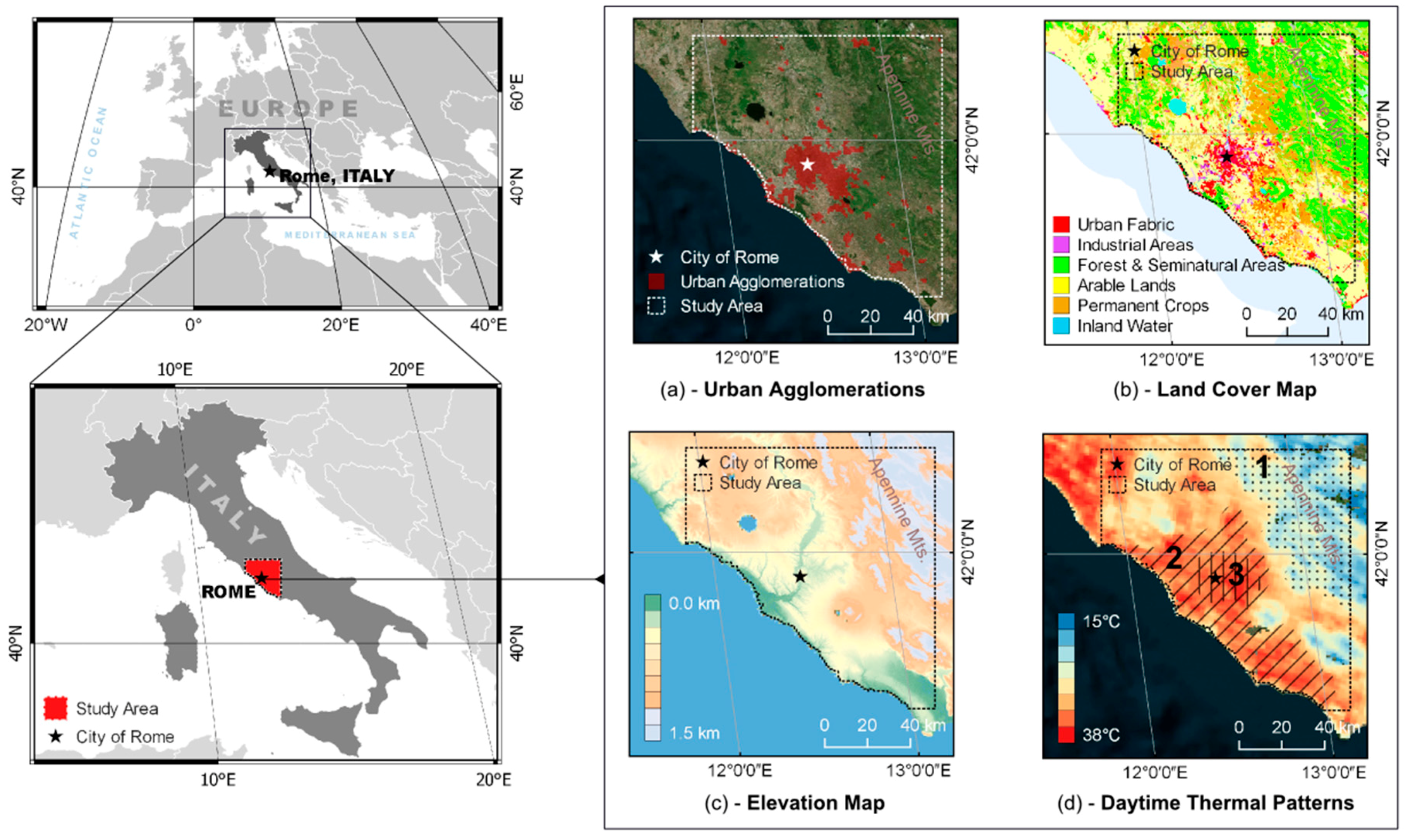
2.1. Study Area
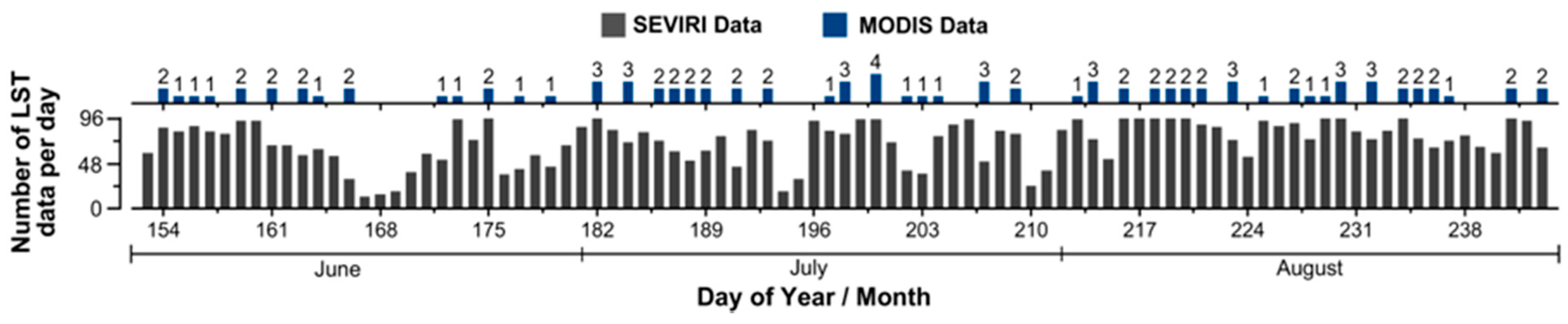
2.2. LST Data
2.3. LST Predictors
3. Method
3.1. SVM-Based DLST Data Generation
3.2. Assessment of Generated DLST Time Series
- Issue 1: the assessment of the method’s accuracy, reliability and consistency.
- Issue 2: the evaluation of the formed DLST spatial patterns.
- Issue 3: the assessment of the potential of the generated DLST time series to emulate the diurnal and seasonal characteristics of the original LST time series.
3.2.1. Accuracy and Consistency Assessment Tests Using a Long Time Series of LST/DLST Data
3.2.2. Test for the Assessment of the Formed Spatial Patterns
3.2.3. Tests for Assessing the DLST Diurnal and Seasonal Features
4. Results and Discussion
4.1. Accuracy and Consistency Assessment
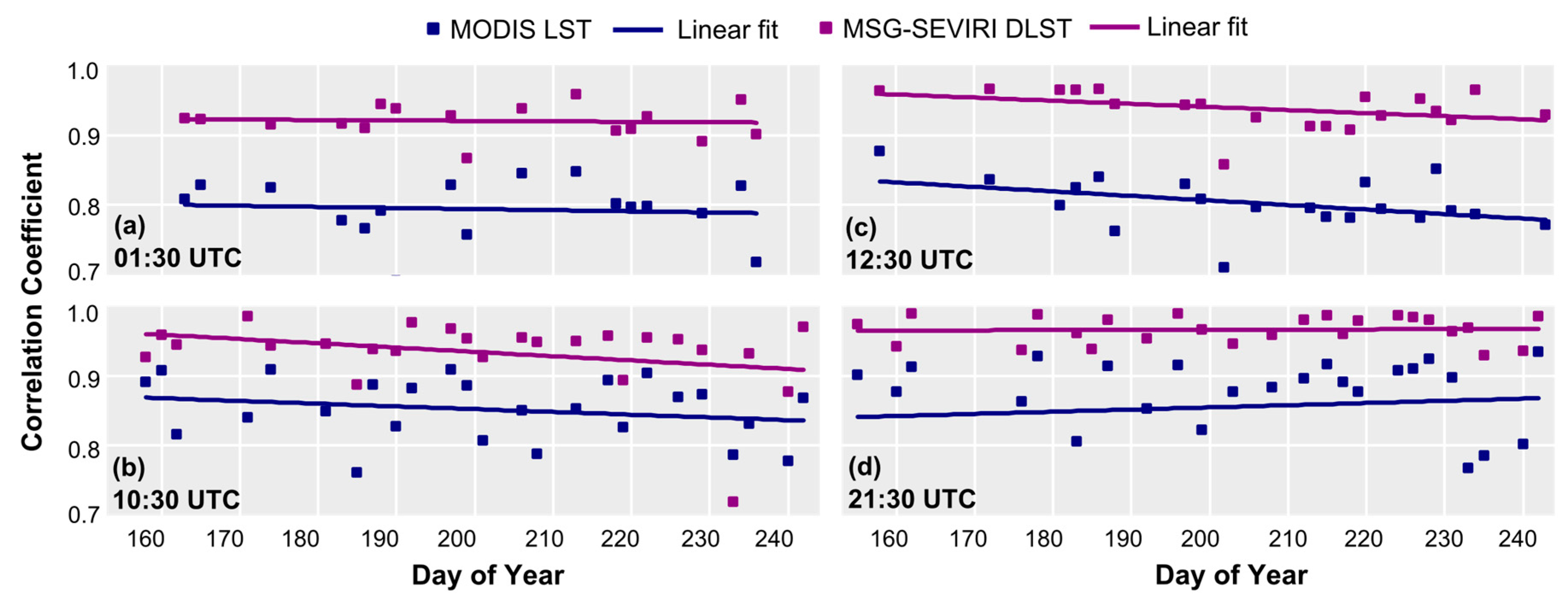
4.1.1. Comparison of Corresponding 1-km MSG3-SEVIRI DLST and MODIS LST Time Series
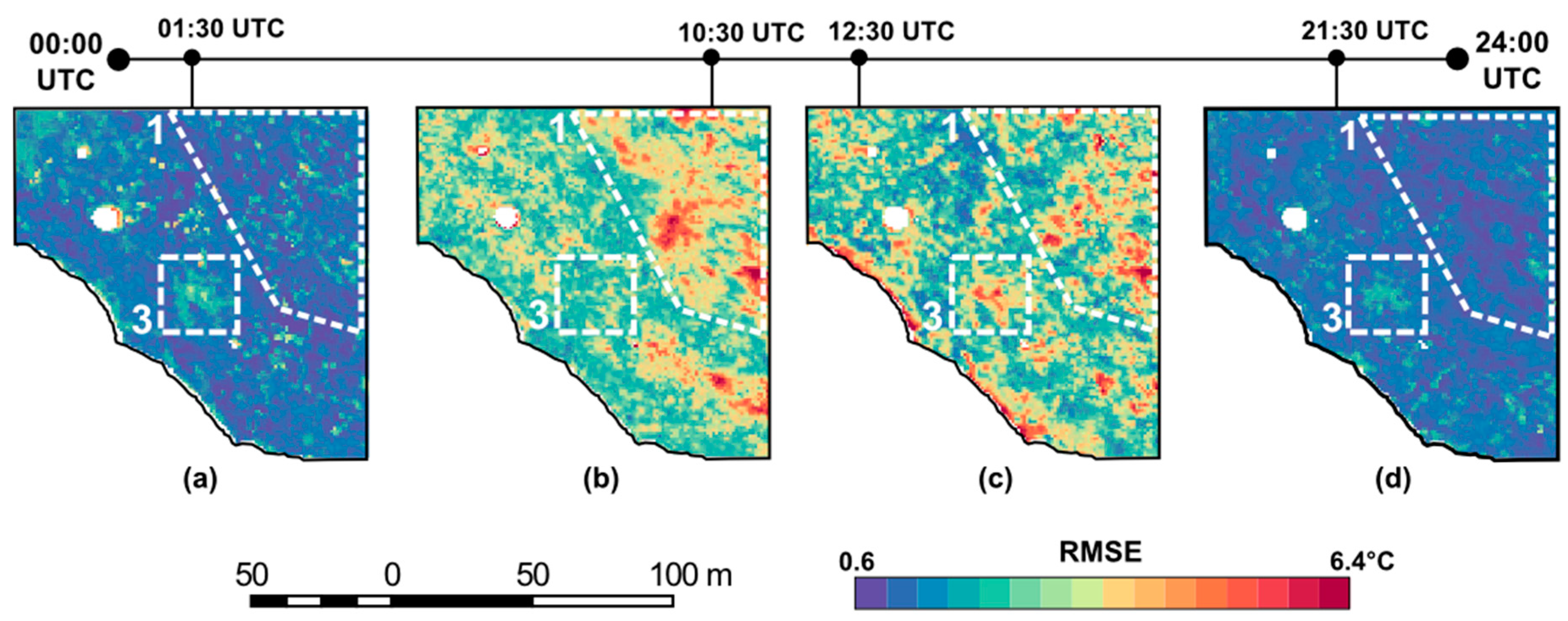
4.1.2. Analysis of RMSE Spatial Distribution
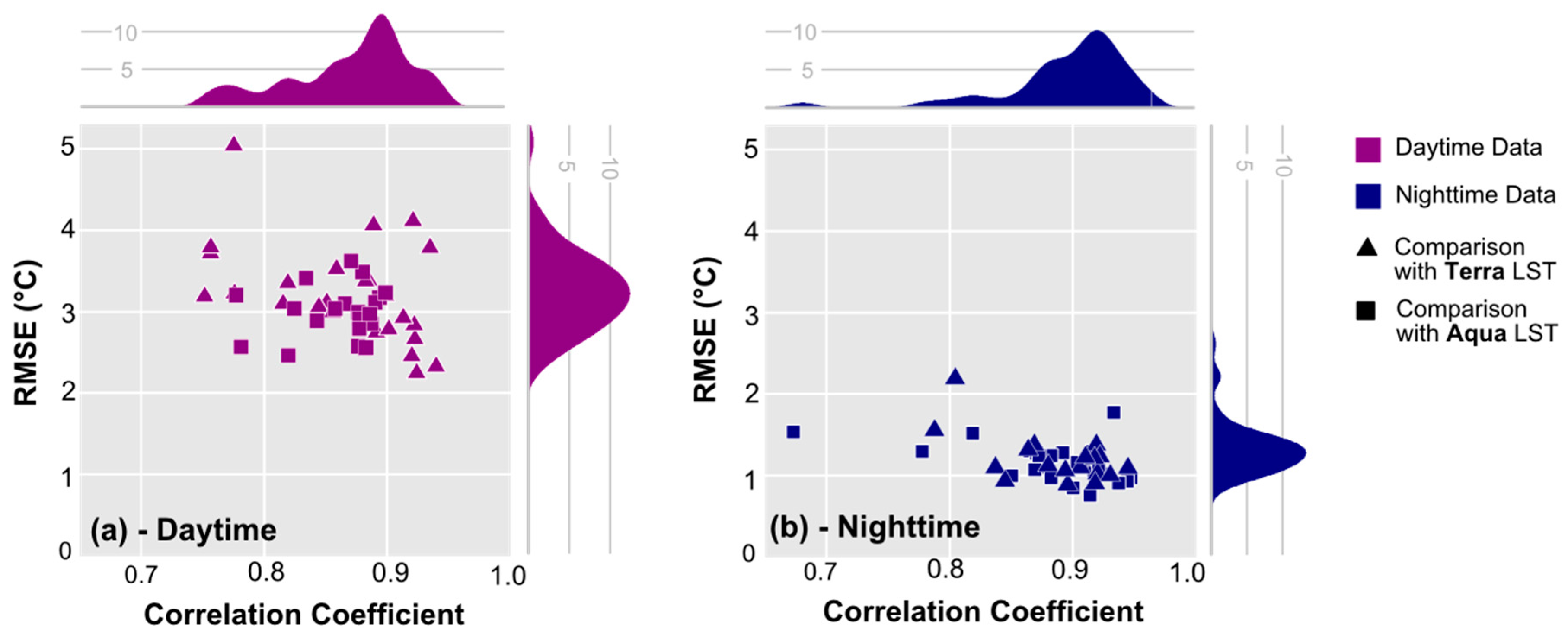
4.1.3. Assessment of the Downscaling Method’s Stability and Consistency
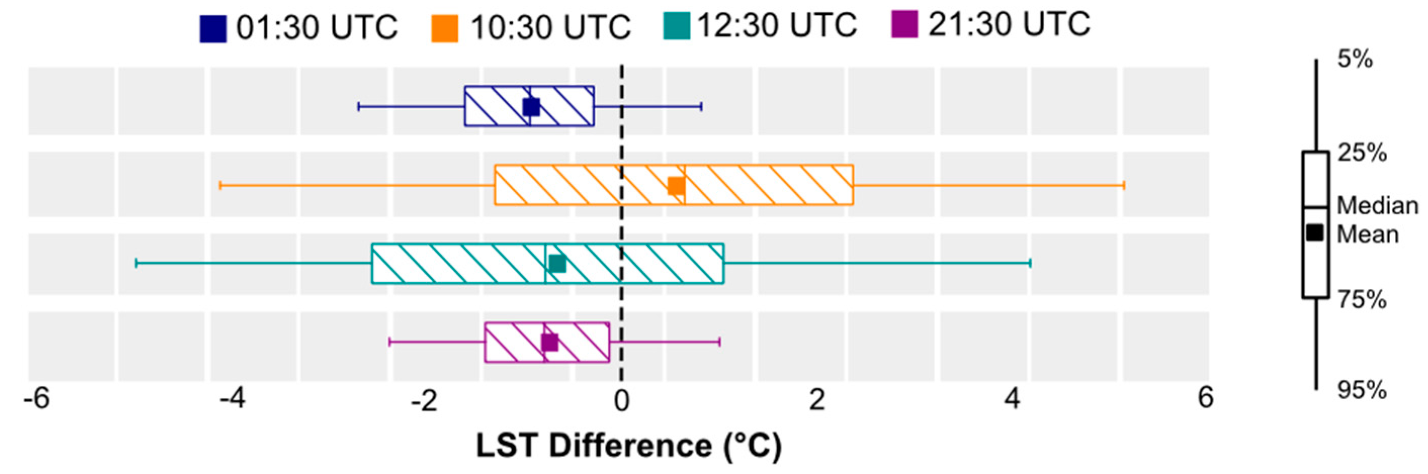
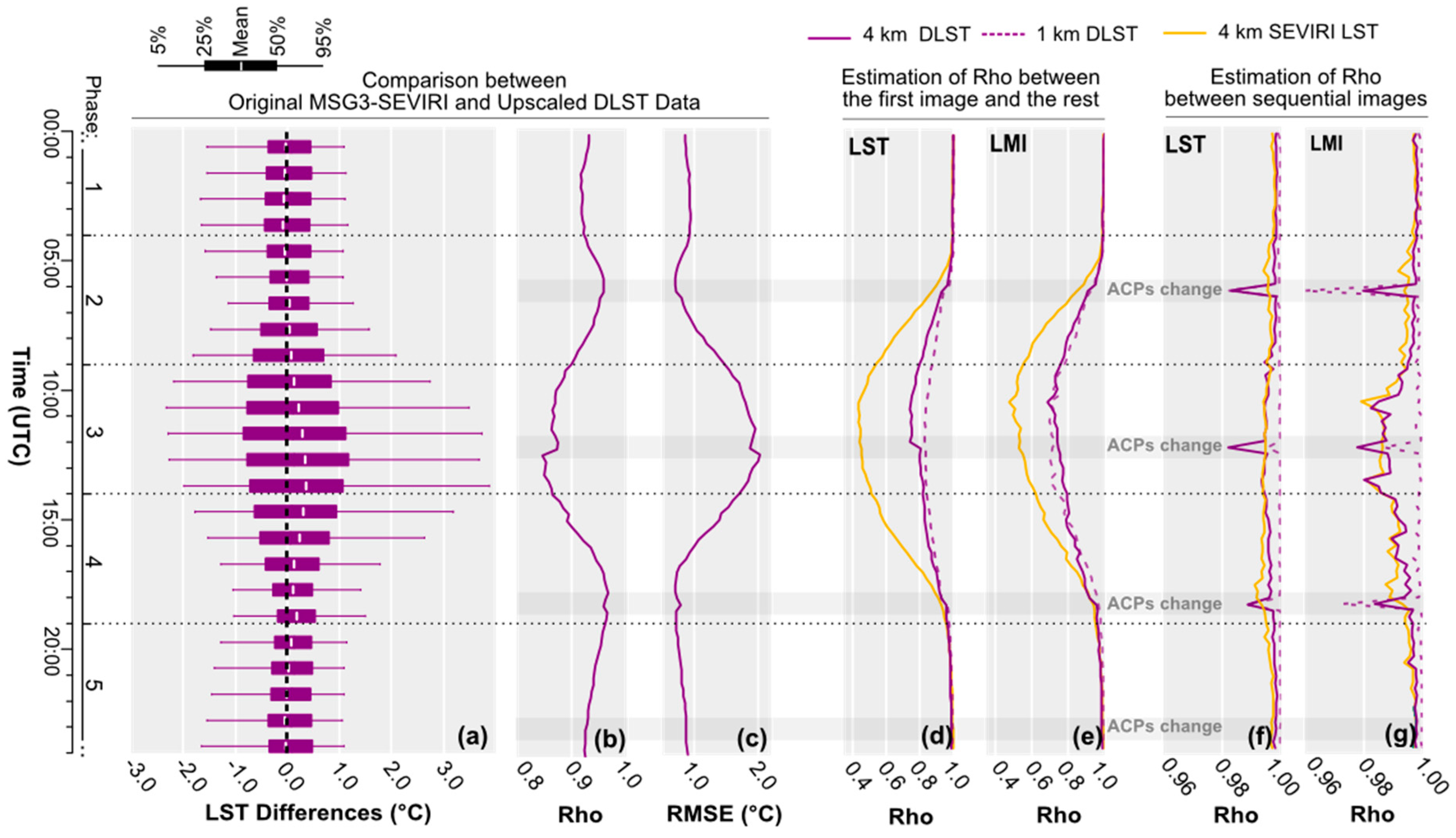
4.1.4. Comparison of MSG3-SEVIRI LST and DLST Time Series
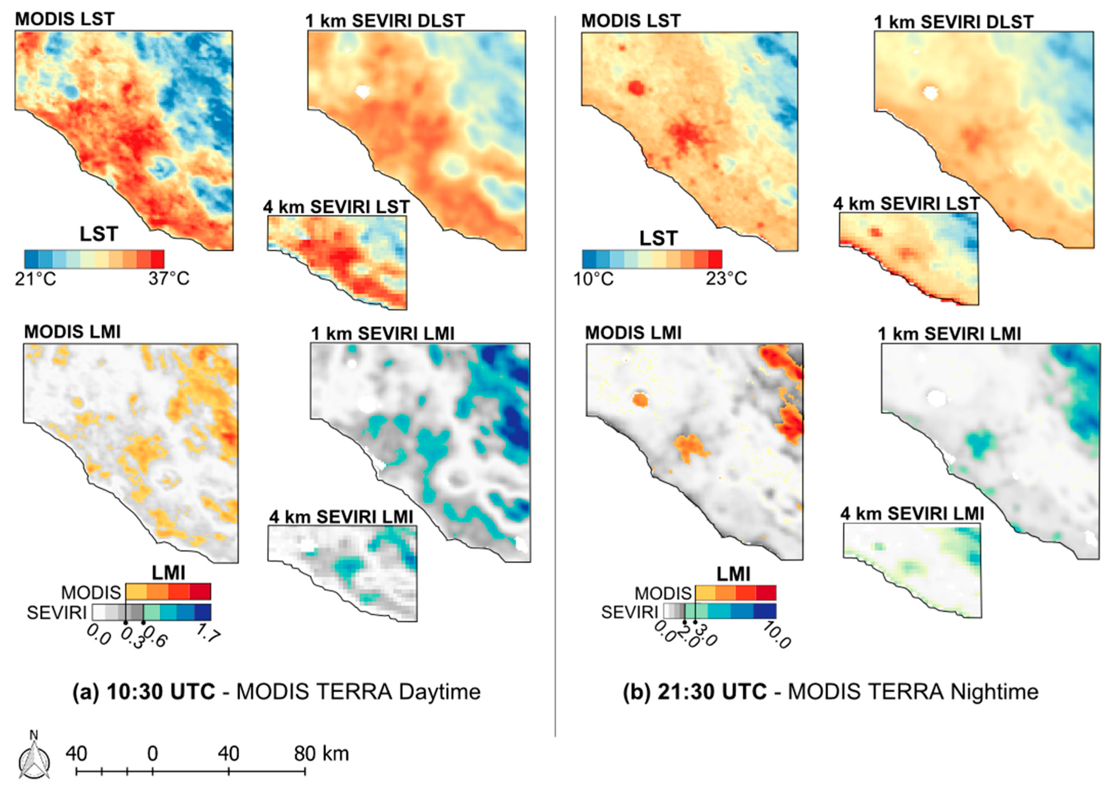
4.2. Assessment of Formed Spatial Patterns
4.3. Assessment of the DLST Spatiotemporal Features
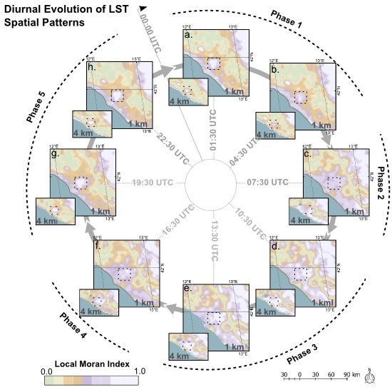
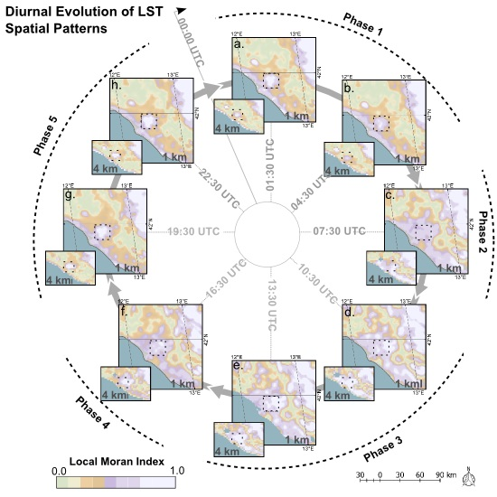
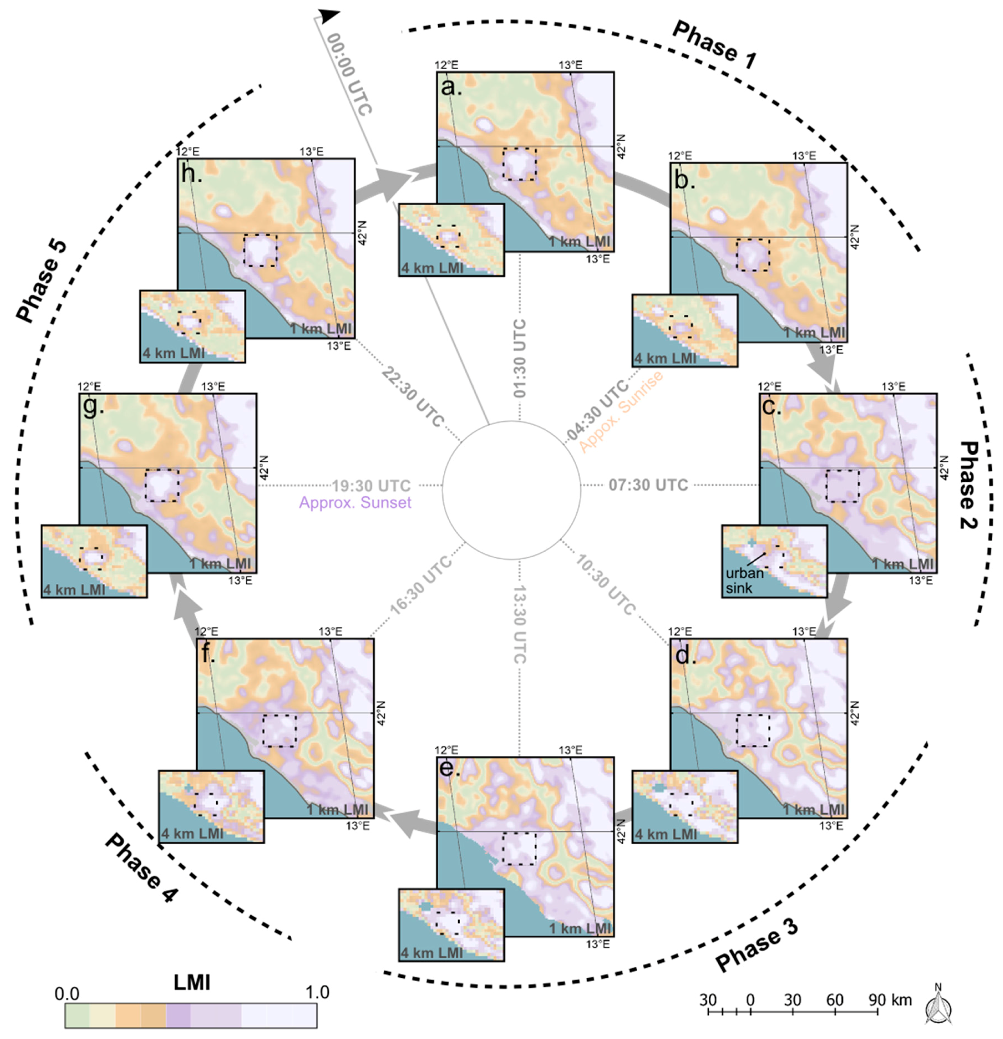
4.3.1. Assessment of the DLST Spatial Pattern Diurnal Evolution
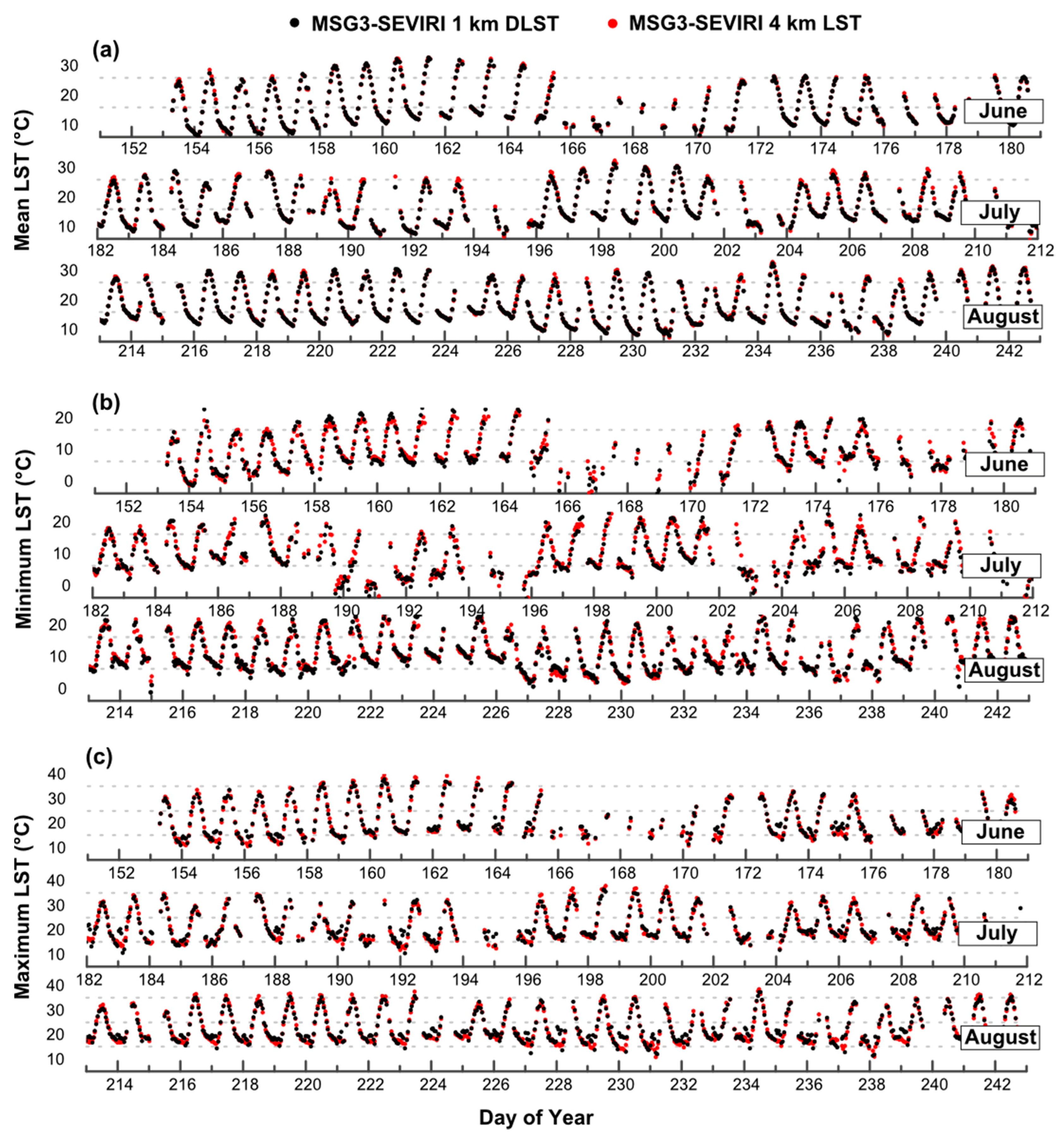
4.3.2. Assessment of the DLST Potential to Emulate LST Temporal Features
5. Conclusions
- The capability of the DLST data to accurately emulate the SUHI diurnal pattern cycle.
- The capability to detect subtle spatial thermal changes during the course of a day.
- The smoothness of the diurnal evolution of the DLST data.
- The consistent performance of the employed downscaling method.
Acknowledgments
Author Contributions
Conflicts of Interest
Abbreviations
| ACPs | Annual Cycle Parameters |
| DLST | Downscaled Land Surface Temperature |
| DOY | Day of Year |
| EVI | Enhanced Vegetation Index |
| IAASARS/NOA | Institute for Astronomy, Astrophysics, Space Applications and Remote Sensing, National Observatory of Athens |
| LMI | Local Moran Index |
| LST | Land Surface Temperature |
| MAST | Mean Annual Surface Temperature |
| MODIS | Moderate Resolution Imaging Spectroradiometer |
| MSG3-SEVIRI | Meteosat Second Generation 3–Spinning Enhanced Visible and Infrared Imager |
| NDVI | Normalized Difference Vegetation Index |
| NNs | Neural Networks |
| Rho | Pearson’s correlation coefficient |
| RMSE | Root-Mean-Square-Error |
| SD | Standard Deviation |
| SRTM | Shuttle Radar Topography Mission |
| SVM | Support Vector Regression Machine |
| SUHI | Surface Urban Heat Island |
| TA | Air Temperature |
| TIR | Thermal Infrared |
| UHI | Urban Heat Island |
| UTC | Coordinated Universal Time |
| VIs | Vegetation Indices |
| VZA | View Zenith Angle |
| YAST | Yearly Amplitude of Surface Temperature |
| ε | Spectral emissivity |
| θ | Phase shift |
References
- Oke, T. The Energetic Basis of the Urban Heat Island. Q. J. R. Meteorol. Soc. 1982, 108, 1–24. [Google Scholar] [CrossRef]
- Mihalakakou, G.; Santamouris, M.; Papanikolaou, N.; Cartalis, C.; Tsangrassoulis, A. Simulation of the Urban Heat Island Phenomenon in Mediterranean Climates. Pure Appl. Geophys. 2004, 161, 429–451. [Google Scholar] [CrossRef]
- Deng, C.; Wu, C. Examining the Impacts of Urban Biophysical Compositions on Surface Urban Heat Island: A Spectral Unmixing and Thermal Mixing Approach. Remote Sens. Environ. 2013, 131, 262–274. [Google Scholar] [CrossRef]
- Taylor, J.; Wilkinson, P.; Davies, M.; Armstrong, B.; Chalabi, Z.; Mavrogianni, A.; Symonds, P.; Oikonomou, E.; Bohnenstengel, S.I. Mapping the Effects of Urban Heat Island, Housing, and Age on Excess Heat-Related Mortality in London. Urban Clim. 2015, 14, 1–12. [Google Scholar] [CrossRef]
- Clinton, N.; Gong, P. MODIS Detected Surface Urban Heat Islands and Sinks: Global Locations and Controls. Remote Sens. Environ. 2013, 134, 294–304. [Google Scholar] [CrossRef]
- Akbari, H.; Davis, S.; Dorsano, S.; Huang, J.; Winnett, S. Cooling Our Communities a Guidebook on Tree Planting and Light-Colored Surfacing; Environmental Protection Agency: Washington, DC, USA, 1992.
- Kim, Y.-H.; Baik, J.-J. Spatial and Temporal Structure of the Urban Heat Island in Seoul. J. Appl. Meteorol. 2005, 44, 591–605. [Google Scholar] [CrossRef]
- Bornstein, R. Observations of the Urban Heat Island Effect in New York City. J. Appl. Meteorol. 1968, 7, 575–582. [Google Scholar] [CrossRef]
- Jones, P.D.; Lister, D.H. The Urban Heat Island in Central London and Urban-Related Warming Trends in Central London since 1900. Weather 2009, 64, 323–327. [Google Scholar] [CrossRef]
- Stathopoulou, M.; Cartalis, C. Daytime Urban Heat Islands from Landsat ETM+ and Corine Land Cover Data: An Application to Major Cities in Greece. Sol. Energy 2007, 81, 358–368. [Google Scholar] [CrossRef]
- Liu, L.; Zhang, Y. Urban Heat Island Analysis Using the Landsat TM Data and ASTER Data: A Case Study in Hong Kong. Remote Sens. 2011, 3, 1535–1552. [Google Scholar] [CrossRef]
- Kato, S.; Yamaguchi, Y. Analysis of Urban Heat-Island Effect Using ASTER and ETM+ Data: Separation of Anthropogenic Heat Discharge and Natural Heat Radiation from Sensible Heat Flux. Remote Sens. Environ. 2005, 99, 44–54. [Google Scholar] [CrossRef]
- Rao, M.K. Remote Sensing of Urban “Heat Islands” from an Environmental Satellite. Bull. Am. Meteorol. Soc. 1972, 53, 647–648. [Google Scholar]
- Price, J. Assessment of the Urban Heat Island Effect through the Use of Satellite Data. Mon. Weather Rev. 1979, 107, 1554–1557. [Google Scholar] [CrossRef]
- Roth, M.; Oke, T.R.; Emery, W.J. Satellite-Derived Urban Heat Islands from Three Coastal Cities and the Utilization of Such Data in Urban Climatology. Int. J. Remote Sens. 1989, 10, 1699–1720. [Google Scholar] [CrossRef]
- Voogt, J.A.; Oke, T. Thermal Remote Sensing of Urban Climates. Remote Sens. Environ. 2003, 86, 370–384. [Google Scholar] [CrossRef]
- Sismanidis, P.; Keramitsoglou, I.; Kiranoudis, C.T. Evaluating the Operational Retrieval and Downscaling of Urban Land Surface Temperatures. IEEE Geosci. Remote Sens. Lett. 2015, 12, 1312–1316. [Google Scholar] [CrossRef]
- Weng, Q. Thermal Infrared Remote Sensing for Urban Climate and Environmental Studies: Methods, Applications, and Trends. ISPRS J. Photogramm. Remote Sens. 2009, 64, 335–344. [Google Scholar] [CrossRef]
- Imhoff, M.L.; Zhang, P.; Wolfe, R.E.; Bounoua, L. Remote Sensing of the Urban Heat Island Effect across Biomes in the Continental USA. Remote Sens. Environ. 2010, 114, 504–513. [Google Scholar] [CrossRef]
- Keramitsoglou, I.; Kiranoudis, C.T.; Ceriola, G.; Weng, Q.; Rajasekar, U. Identification and Analysis of Urban Surface Temperature Patterns in Greater Athens, Greece, Using MODIS Imagery. Remote Sens. Environ. 2011, 115, 3080–3090. [Google Scholar] [CrossRef]
- Li, Z.-L.; Tang, B.-H.; Wu, H.; Ren, H.; Yan, G.; Wan, Z.; Trigo, I.F.; Sobrino, J.A. Satellite-Derived Land Surface Temperature: Current Status and Perspectives. Remote Sens. Environ. 2013, 131, 14–37. [Google Scholar] [CrossRef]
- Zakšek, K.; Oštir, K. Downscaling Land Surface Temperature for Urban Heat Island Diurnal Cycle Analysis. Remote Sens. Environ. 2012, 117, 114–124. [Google Scholar] [CrossRef]
- Keramitsoglou, I.; Kiranoudis, C.T.; Weng, Q. Downscaling Geostationary Land Surface Temperature Imagery for Urban Analysis. IEEE Geosci. Remote Sens. Lett. 2013, 10, 1253–1257. [Google Scholar] [CrossRef]
- Bechtel, B.; Zakšek, K.; Hoshyaripour, G. Downscaling Land Surface Temperature in an Urban Area: A Case Study for Hamburg, Germany. Remote Sens. 2012, 4, 3184–3200. [Google Scholar] [CrossRef]
- Weng, Q.; Fu, P. Modeling Diurnal Land Temperature Cycles over Los Angeles Using Downscaled GOES Imagery. ISPRS J. Photogramm. Remote Sens. 2014, 97, 78–88. [Google Scholar] [CrossRef]
- Zhan, W.; Chen, Y.; Zhou, J.; Wang, J.; Liu, W.; Voogt, J.; Zhu, X.; Quan, J.; Li, J. Disaggregation of Remotely Sensed Land Surface Temperature: Literature Survey, Taxonomy, Issues, and Caveats. Remote Sens. Environ. 2013, 131, 119–139. [Google Scholar] [CrossRef]
- Agam, N.; Kustas, W.P.; Anderson, M.C.; Li, F.; Neale, C.M.U. A Vegetation Index Based Technique for Spatial Sharpening of Thermal Imagery. Remote Sens. Environ. 2007, 107, 545–558. [Google Scholar] [CrossRef]
- Kustas, W.P.; Norman, J.M.; Anderson, M.C.; French, A.N. Estimating Subpixel Surface Temperatures and Energy Fluxes from the Vegetation Index–radiometric Temperature Relationship. Remote Sens. Environ. 2003, 85, 429–440. [Google Scholar] [CrossRef]
- Inamdar, A.K.; French, A.; Hook, S.; Vaughan, G.; Luckett, W. Land Surface Temperature Retrieval at High Spatial and Temporal Resolutions over the Southwestern United States. J. Geophys. Res. 2008, 113, 1–18. [Google Scholar] [CrossRef]
- Sun, D.; Kafatos, M. Note on the NDVI-LST Relationship and the Use of Temperature-Related Drought Indices over North America. Geophys. Res. Lett. 2007, 34, 1–4. [Google Scholar] [CrossRef]
- Jeganathan, C.; Hamm, N.A.S.; Mukherjee, S.; Atkinson, P.M.; Raju, P.L.N.; Dadhwal, V.K. Evaluating a Thermal Image Sharpening Model over a Mixed Agricultural Landscape in India. Int. J. Appl. Earth Obs. Geoinf. 2011, 13, 178–191. [Google Scholar] [CrossRef]
- Wu, P.; Shen, H.; Zhang, L.; Göttsche, F.-M. Integrated Fusion of Multi-Scale Polar-Orbiting and Geostationary Satellite Observations for the Mapping of High Spatial and Temporal Resolution Land Surface Temperature. Remote Sens. Environ. 2015, 156, 169–181. [Google Scholar] [CrossRef]
- Weng, Q.; Fu, P.; Gao, F. Generating Daily Land Surface Temperature at Landsat Resolution by Fusing Landsat and MODIS Data. Remote Sens. Environ. 2014, 145, 55–67. [Google Scholar] [CrossRef]
- Bechtel, B. Robustness of Annual Cycle Parameters to Characterize the Urban Thermal Landscapes. IEEE Geosci. Remote Sens. Lett. 2012, 9, 876–880. [Google Scholar] [CrossRef]
- Bechtel, B. A New Global Climatology of Annual Land Surface Temperature. Remote Sens. 2015, 7, 2850–2870. [Google Scholar] [CrossRef]
- Bechtel, B.; Böhner, J.; Zakšek, K.; Wiesner, S. Downscaling of Diumal Land Surface Temperature Cycles for Urban Heat Island Monitoring. In Proceedings of the Joint Urban Remote Sensing Event, Sao Paolo, Brazil, 21–23 April 2013.
- Verbesselt, J.; Zeileis, A.; Herold, M. Near Real-Time Disturbance Detection Using Satellite Image Time Series. Remote Sens. Environ. 2012, 123, 98–108. [Google Scholar] [CrossRef]
- Tan, J.; Zheng, Y.; Tang, X.; Guo, C.; Li, L.; Song, G.; Zhen, X.; Yuan, D.; Kalkstein, A.J.; Li, F. The Urban Heat Island and Its Impact on Heat Waves and Human Health in Shanghai. Int. J. Biometeorol. 2010, 54, 75–84. [Google Scholar] [CrossRef] [PubMed]
- Lo, C.P.; Quattrochi, D.A.; Luvall, J.C. Application of High-Resolution Thermal Infrared Remote Sensing and GIS to Assess the Urban Heat Island Effect. Int. J. Remote Sens. 2010, 18, 287–304. [Google Scholar] [CrossRef]
- Julien, Y.; Sobrino, J.A. The Yearly Land Cover Dynamics (YLCD) Method: An Analysis of Global Vegetation from NDVI and LST Parameters. Remote Sens. Environ. 2009, 113, 329–334. [Google Scholar] [CrossRef]
- Sismanidis, P.; Keramitsoglou, I.; Kiranoudis, C.T. A Satellite-Based System for Continuous Monitoring of Surface Urban Heat Islands. Urban Clim. 2015, 14, 141–153. [Google Scholar] [CrossRef]
- Trigo, I.F.; Monteiro, I.T.; Olesen, F.; Kabsch, E. An Assessment of Remotely Sensed Land Surface Temperature. J. Geophys. Res. 2008, 113, D17108. [Google Scholar] [CrossRef]
- Rabus, B.; Eineder, M.; Roth, A.; Bamler, R. The Shuttle Radar Topography Mission-A New Class of Digital Elevation Models Acquired by Spaceborne Radar. ISPRS J. Photogramm. Remote Sens. 2003, 57, 241–262. [Google Scholar] [CrossRef]
- Arino, O.; Gross, D.; Ranera, F.; Bourg, L.; Leroy, M.; Bicheron, P.; Latham, J.; Di Gregorio, A.; Brockman, C.; Witt, R.; et al. GlobCover: ESA Service for Global Land Cover from MERIS. In Geoscience and Remote Sensing Symposium; IEEE: Barcelona, Spain, 2007; pp. 2412–2415. [Google Scholar] [CrossRef]
- Mountrakis, G.; Im, J.; Ogole, C. Support Vector Machines in Remote Sensing: A Review. ISPRS J. Photogramm. Remote Sens. 2010, 66, 259–247. [Google Scholar] [CrossRef]
- Anselin, L. Local Indicators of Spatial Association—LISA. Geogr. Anal. 1995, 27, 93–115. [Google Scholar] [CrossRef]
- Voogt, J.; Oke, T. Complete Urban Surface Temperatures. J. Appl. Meteorol. 1997, 36, 1117–1132. [Google Scholar] [CrossRef]
- Fabrizi, R.; Bonafoni, S.; Biondi, R. Satellite and Ground-Based Sensors for the Urban Heat Island Analysis in the City of Rome. Remote Sens. 2010, 2, 1400–1415. [Google Scholar] [CrossRef]


| Type | LST Predictors |
|---|---|
| Topography Data | Altitude, slope, aspect N, aspect S, aspect W and aspect E |
| Land Cover Data | Water bodies, urban areas, agricultural areas, and vegetated areas |
| Emissivity Data | 8-day 11-μm and 12-μm emissivities (MOD11A2) |
| Vegetation Indices | 16-day NDVI and EVI (MOD13A2) |
| LST Annual Climatology Data | YAST, MAST and θ |
| Issue | # | Aim | Tests |
|---|---|---|---|
| Issue 1 | 1 | Quantification of differences between MSG3-SEVIRI DLST-MODIS LST time series. | Statistical measures at fine resolution (1 km). |
| 2 | Downscaling performance with respect to land cover type. | RMSE spatial distribution. | |
| 3 | Downscaling method’s consistency assessment. | Image-to-image analysis between MSG-SEVIRI DLST-MODIS LST. | |
| 4 | Assessment of DLST when no coincident MODIS data are available. | Statistical measures at original resolution (4 km). | |
| Issues 2 & 3 | 5 | Assessment of formed pattern’s shape, size and location. | DLST and MODIS LST Local Moran Indices (LMI) comparison. |
| 6 | Compliance of DLST and original LST pattern diurnal evolution. | LMI juxtaposition and visual inspection. | |
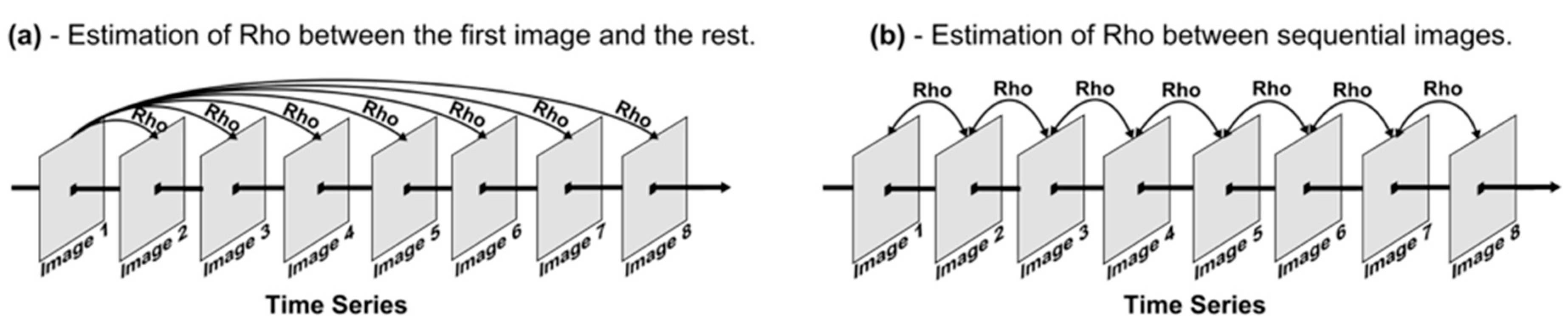
| 7 | Magnitude of diurnal spatial change. | Similarity between the first image of the day and the remaining 95. | |
| 8 | Smoothness of DLST diurnal spatial change/artifact formation due to ACPs’ sudden change. | Similarity between sequential quarter-hourly images. | |
| 9 | Preservation of original radiometry. | Min/mean/max LST-DLST value comparison. | |
| 10 | DLST potential to emulate the spatial changes due to seasonal effects. | Similarity between sequential images. |
| Statistical Measures | 01:30 UTC | 10:30 UTC | 12:30 UTC | 21:30 UTC |
|---|---|---|---|---|
| Mean Difference | −0.46 | +1.10 | −0.20 | −0.25 |
| Variance | 1.41 | 9.10 | 8.96 | 1.38 |
| SD | 1.19 | 3.02 | 2.99 | 1.18 |
| RMSE | 1.27 | 3.21 | 3.00 | 1.20 |
| Rho | 0.88 | 0.85 | 0.86 | 0.91 |
© 2016 by the authors; licensee MDPI, Basel, Switzerland. This article is an open access article distributed under the terms and conditions of the Creative Commons by Attribution (CC-BY) license (http://creativecommons.org/licenses/by/4.0/).
Share and Cite
Sismanidis, P.; Keramitsoglou, I.; Kiranoudis, C.T.; Bechtel, B. Assessing the Capability of a Downscaled Urban Land Surface Temperature Time Series to Reproduce the Spatiotemporal Features of the Original Data. Remote Sens. 2016, 8, 274. https://doi.org/10.3390/rs8040274
Sismanidis P, Keramitsoglou I, Kiranoudis CT, Bechtel B. Assessing the Capability of a Downscaled Urban Land Surface Temperature Time Series to Reproduce the Spatiotemporal Features of the Original Data. Remote Sensing. 2016; 8(4):274. https://doi.org/10.3390/rs8040274
Chicago/Turabian StyleSismanidis, Panagiotis, Iphigenia Keramitsoglou, Chris T. Kiranoudis, and Benjamin Bechtel. 2016. "Assessing the Capability of a Downscaled Urban Land Surface Temperature Time Series to Reproduce the Spatiotemporal Features of the Original Data" Remote Sensing 8, no. 4: 274. https://doi.org/10.3390/rs8040274
APA StyleSismanidis, P., Keramitsoglou, I., Kiranoudis, C. T., & Bechtel, B. (2016). Assessing the Capability of a Downscaled Urban Land Surface Temperature Time Series to Reproduce the Spatiotemporal Features of the Original Data. Remote Sensing, 8(4), 274. https://doi.org/10.3390/rs8040274